Bottom-up carbon dots: purification, single-particle dynamics, and electronic structure

Abstract

The physico-chemical properties of ‘bottom-up’ carbon dots synthesized from small molecules feature both generalities, such as sp²-networked carbon and core-surface energy transfer, and heterogeneities, due to the unpredictable location of heteroatoms and often non-crystalline structure. Here we focus our review on three aspects of these systems: (1) coupling characterization with bottom-up synthesis to identify and remove confounding byproducts such as small molecules or hydrogen-rich polymers; (2) single-particle characterization to obtain unambiguous information on carbon dots and highlight the distribution of properties around the ensemble average; (3) electronic structure of carbon dots and how it can help elucidate the origin of important properties such as optical absorption and fluorescence from a heterogeneous ensemble of carbon dots.

---

1 Introduction

Since the late 1980s, different nanoscale carbon materials have excited the imagination of the nanoscience community: buckyballs,¹ carbon nanotubes,² graphene and graphene oxide sheets,³ and most recently carbon dots.⁴ Carbon dots are nanometer-size particles rich in sp² networked carbon, but also contain heteroatoms either due to their top-down synthesis from oxidized graphite particles, or bottom-up synthesis from small organic molecules. Top-down carbon dots often show multilayered graphenic structure, while bottom-up carbon dots typically are more amorphous materials due to the presence of heteroatoms such as nitrogen in their bulk, presumably following the condensation of smaller carbon sheets into dots.⁵ Carbon dots cover an interesting regime where molecular and bulk quantum effects can compete.⁶

In this review, we focus on the synthesis, single particle-verified properties, and electronic structure of bottom-up carbon dots with sp²-carbon rich cores, as species closely related to top-down carbon dots. Bottom-up carbon dots allow a great variety of heteroatom doping, but the relatively harsh and uncontrolled conditions of pyrolysis-, ablation- or solvothermal reaction at high temperature produce heterogeneous dots with a size distribution and unpredictable defects. The name ‘carbon dot’ has also been applied to other materials, such as polyester nanospheres made by microwave synthesis, shown to lack the sp² network.⁷ In addition, study of bottom-up carbon dots has been complicated by the presence of many small-molecule byproducts;^8,9 we do not include such CH₂-rich (mainly sp³) materials and small molecules under ‘bottom-up’ carbon dots and focus instead on materials in the 3–10 nm size where Raman G-bands,¹⁰ electron microscopy,¹¹ scanning tunneling microscopy (STM) bandgap measurements,¹² or single molecule techniques¹³ have verified the sp² networked nature of the nanoparticles, whether they are mainly crystalline (top-down syntheses) or mainly amorphous (bottom-up syntheses).

As nano-size particles with good biocompatibility, straight-forward synthesis, high solubility when properly surface-modified, strong optical absorption (extinction up to 10⁶ M⁻¹ cm⁻¹), and interesting fluorescence properties (generally blue to yellow, with red fluorescence less certain), carbon dots have been proposed for myriad applications in imaging, cell-based therapies, sensors, and catalysis. These applications have been reviewed in depth recently in the literature,⁴ and will not be considered in this review. Instead, we will focus here on the triptych of synthesis-purification, single-particle imaging, and electronic structure on which the physical chemistry knowledge of bottom-up carbon dots is built.

Many basic concepts from organic synthesis come into play in identifying oligomeric precursors and byproducts that can interfere with carbon dot spectroscopy,¹⁴ and analytical chemistry provides techniques that allow resolution of carbon dots,¹⁵ sometimes several fractions with different optical properties, from precursors and byproducts so the genuine carbon dot can be characterized; single particle techniques such as confocal fluorescence microscopy, scanning tunneling microscopy, ultrafast single particle spectroscopy, atomic force microscopy, and transmission electron microscopy allow reliable identification of carbon dots based on physical properties such as size, crystallinity, optical bandgaps, and electrical properties;^16,17 finally, electronic structure calculations, difficult but valuable for such large systems can tell us about the origin of optical properties from likely surface defects contributing to fluorescence, to core-surface coupling that blue-shifts fluorescence of surface chromophores, to internal conversion or intersystem crossing processes that relax energy within carbon dots and affect their quantum yields.¹⁸

Intrinsically heterogeneous nanomaterials such as carbon dots are best studied by this three-fold combination of extensive purification, single particle analysis, and electronic structure theory approaches to achieve a better basic understanding of their properties and provide insights how to tailor syntheses to produce materials that while remaining heterogeneous, have desirable properties either on average (e.g. bio-optical applications) or in their outliers (e.g. catalytic applications).

2 Bottom-up synthesis and purification

2.1 Bottom-up techniques

Bottom-up synthesis methods play a crucial role in the field of carbon dots,¹⁹ where organic small molecules such as citric acid, phenylenediamine, urea, and glucose are commonly employed as precursors. These molecules undergo various synthesis techniques such as hydro/solvothermal treatment, microwave methods, and template approaches to form carbon dots. However, the optical properties of the resultant carbon dots can be obscured by the presence of small fluorescent molecules formed during synthesis. Consequently, analyses based on impure carbon dots may yield misleading conclusions. To mitigate such inaccuracies, purification methods including dialysis, gel electrophoresis, and size-exclusion and gel chromatography are routinely utilized. These techniques effectively separate carbon dots from residual small molecules and ensure the integrity of subsequent optical property evaluations and application assessments.

In the characterization phase, structural and compositional analyses play a pivotal role. Techniques such as transmission electron microscopy (TEM), atomic force microscopy (AFM), mass spectrometry (MS), X-ray diffraction (XRD), nuclear magnetic resonance (NMR) spectroscopy, Fourier-transform infrared spectroscopy (FTIR), and X-ray photoelectron spectroscopy (XPS) are employed. These methods provide insights into the morphology, crystallinity, chemical structure, and elemental composition of carbon dots, crucial for understanding their properties and optimizing their performance in various applications.

Hydro/solvothermal synthesis involves the use of water or organic solvent in a high-pressure, high-temperature environment to facilitate the formation of carbon dots.²⁰ The process occurs in a sealed vessel, such as an autoclave, where the aqueous/organic solution containing carbon precursors undergoes thermal decomposition, polymerization, and graphitization to produce carbon dots in a high-pressure, high-temperature (150–250 °C) environment. The choice of precursors, reaction conditions, and solvents can significantly influence the size, morphology, and functionalization of the resulting carbon dots. The primary advantages of this method include its simplicity and cost-effectiveness.

Microwave-assisted synthesis has emerged as an efficient method for the production of carbon dots.²¹ Microwave-assisted synthesis utilizes microwave radiation to heat a reaction mixture quickly and uniformly. This approach reduces thermal gradients, enhance reaction rates, and reduce synthesis times, leading to better control over the reaction conditions and hence improving the consistency, reproducibility, and overall quality of the carbon dots produced. The drawback over solvothermal synthesis is that the milder (low pressure) conditions may not promote the formation of sp²-hybridized lattices, leading instead to the formation of polymer nanoparticles.

Pyrolysis involves heating organic precursors in a controlled environment to decompose them into carbon-rich materials.²² The process typically occurs at temperatures ranging from 300 °C to 900 °C under an inert atmosphere (e.g., nitrogen or argon) to minimize oxidation.²³ Pyrolysis is an efficient technique for converting small organic molecules into carbon nanoparticles, making it suitable for large-scale production and diverse applications, due to its simplicity and scalability.²⁴

Template synthesis involves the use of a template material like silica nanospheres to guide the formation of carbon dots.^25,26 The template provides a specific shape or structure that the carbon precursors adhere to or fill, thereby influencing the final morphology and properties of the carbon dots, but also preventing aggregation of the nanosized carbon dots during pyrolysis. After the synthesis, the template is usually removed by etching with NaOH or HF solution,^27,28 leaving behind the desired carbon dots.

Electrochemical bottom-up synthesis of carbon dots oxidizes and polymerizes small organic precursors, such as citric acid, ethanol, glucose, or amino acids, to form carbonaceous nanoparticles. This process occurs in an electrochemical cell comprising two electrodes submerged in an electrolyte solution containing the carbon precursors.^29,30

2.2 Problems in bottom-up synthesis

Although researchers have made high quantum yield, biocompatible, and photostable carbon dots by means of the synthesis methods discussed above, small molecules existing in the reaction are a big issue for bottom-up carbon dots, and can confound the origin of fluorescence and other optical properties. In the citric acid–amine system, carbon dots synthesized from citric acid and ethylenediamine appear to exhibit a sharp absorption band, high quantum yield values, and excitation-independent photoluminescence (PL) when excited through that band, but a molecular fluorophore is the likely origin.⁷ Although various models have been proposed to explain the observed emission properties, such as energy transfer among different fluorophores embedded within a carbonaceous scaffold, surface-mediated photoluminescence, and aggregation-mediated photoluminescence, the discovery of the highly emissive citrazinic acid derivative imidazo[1,2-a]pyridine-7-carboxylic acid, 1,2,3,5-tetrahydro-5-oxo (IPCA) as a byproduct of this synthesis raises questions about the true nature of this emission.^31,32 This type of reaction forming novel blue emissive compounds can also be found in the reaction between all citric acid and α,β-amines, β-amino alcohols, and β-amino thiols.^33,34

A similar situation occurred when ortho-, meta-, and para-phenylenediamine (OPD, MPD and PPD) are used as precursor for making multicolor carbon dots.³⁵ Time-resolved electron paramagnetic resonance spectroscopy (TREPR) and fluorescence correlation spectroscopy (FCS) characterization have revealed that the unusually high fluorescence quantum yield originates mainly from small molecules with sizes of less than 10 A formed during early stages of the hydrothermal synthesis (Fig. 1).⁸ The red/green/blue fluorescent small molecules are formed by the condensation reaction of aminobenzene and the reaction between the aminobenzene and ethanol in oxygenated solvents.¹⁴

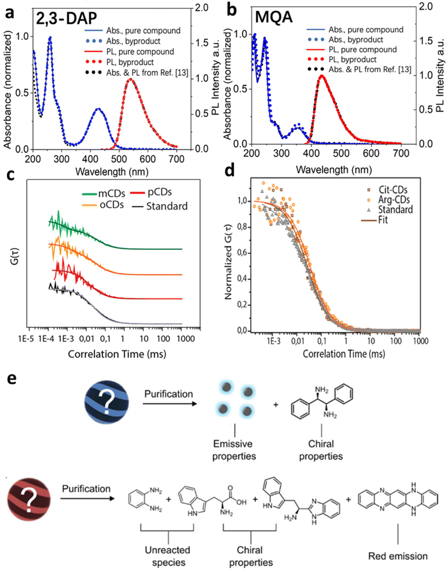Fig. 1 Small molecular byproducts in the bottom-up synthesis of carbon dots. (a and b) UV-vis absorption spectra and emission spectra of commercially pure compounds 2,3-diaminophenazine (2,3-DAP) and 2-methylquinolin-7-amine (MQA), low molecular weight product from bottom-up synthesis,¹⁴ and spectra mis-assigned to o-carbon dots and m-carbon dots in ref. 35. (c) Normalized FCS curves with fits for solutions containing byproducts and o-carbon dots (yellow), m-carbon dots (green), and p-carbon dots (red), with Coumarin 503 as a standard for comparison (adapted with permission from ref. 8). The rapid diffusion indicates that fluorescence originates from small molecules, not carbon dots. (d) Normalized FCS curves for citrate Cit-carbon dots (brown), Arg-carbon dots (orange), and Coumarin 153 (gray), resulting in a similar conclusion (adapted with permission from ref. 34). (e) Details of the structure and properties of species identified after purification. The chiroptical properties result not from carbon dots, but from unreacted precursors and their small-molecule derivatives (adapted with permission from ref. 36).

2.3 Purification – obligatory for carbon dots

Above all, purification is crucial in the field of bottom-up systems where small-molecule absorption and fluorescence are too easily mistaken for the optical properties of carbon dots.

Dialysis is a separation technique³⁷ that operates based on the principle of selective permeability of a dialysis membrane. In this process, a solution containing carbon dots is placed inside a dialysis tubing or membrane, which is then submerged in a larger volume of water or buffer solution. The membrane allows small molecules, ions, and impurities to pass through while retaining larger molecules such as carbon dots. Over time, the removal of unwanted substances and the purification of the carbon dots are achieved.

Membranes are characterized by their molecular weight cut-off (MWCO), which determines the size of molecules that can pass through. Choosing a dialysis membrane with a suitable MWCO is critical for sufficient purification.⁹ Common MWCOs range from 1 kDa to 50 kDa, depending on the size of the carbon dots and the molecular weight of impurities. The duration is also important for a successful dialysis.³⁷ For bottom-up carbon dots that are not adequately dialyzed to separate small precursor molecules, analysis of the chemical compositions or the fluorescence properties of the samples collected only leads to meaningless and confusing conclusions.

Dialysis membranes are typically composed of cellulose ester (CE) or regenerated cellulose (RC). The choice of membrane material influences its resistance to various organic solvents. Cellulose ester membranes are particularly sensitive to organic solvents. Strong polar solvents such as acetone, methyl ethyl ketone, or dioxane can cause irreparable damage to CE membranes. However, lower alcohols like methanol, ethanol, and isopropanol can be used with CE membranes for short exposure times or at low concentrations. In contrast, regenerated cellulose membranes exhibit good chemical resistance to a broad range of solvents, including hydrocarbons, halogenated hydrocarbons, alcohols, ketones, esters, oxides, and solvents containing nitrogen. RC membranes are therefore more versatile and durable in carbon dot dialysis applications.

Size-exclusion columns also operate on the principle of size-based separation. A sample containing carbon dots and other components is introduced into a column packed with a porous stationary phase, often composed of cross-linked polymer beads. As the sample flows through the column, smaller molecules diffuse into the pores of the stationary phase, while larger carbon dots, are excluded from the pores and elute faster. This size-based separation allows for the isolation of carbon dots from other contaminants and byproducts.

Materials such as Sephadex or Bio-Gel are employed as a stationary phase,³⁸ providing a range of pore sizes suitable for different molecular weights and sizes. Due to the different solubility of different carbon dots species in organic solvent and water, Sephadex columns can be used in either organic or aqueous phases, such as Sephadex LH-20 for most organic solvents,³⁹ and G100 for water,⁴⁰ providing universal purification for both hydrophilic and hydrophobic carbon dots.

Silica gel column chromatography is a widely used technique for the separation and characterization of carbon dots.⁴¹ Carbon dots with fair solubility in organic solvents are appropriate for silica gel columns to separate different fractions based on the difference in polarity. This method leverages the differences in the physical and chemical interactions between carbon dots and the silica gel stationary phase to purify and fractionate carbon dots based on their size, surface properties, and chemical composition.

Gel electrophoresis was used for purification of the very first batch of carbon dots in 2004.⁴² Gel electrophoresis involves the application of an electric field across a gel matrix, separating particles based on their size and charge. Carbon dots, depending on their surface charge (e.g. from carboxylates) and size, migrate through the gel at different rates, allowing for their separation from other particles, as well as neutral small molecule impurities. The gel matrix acts as a molecular sieve, with smaller particles with more charge migrating faster through the pores while larger particles with less charge encountering more resistance and moving slower.⁴³

2.4 Structural and compositional analysis

Transmission Electron Microscopy (TEM) enables a direct check for the existence of carbon dots because single small molecules are below the resolution and carbon dots show decent contrast in TEM images. TEM is also widely used to determine the size distribution, shape, and morphology of carbon dots, e.g. whether carbon dots have amorphous or crystalline structure. High-resolution TEM (HRTEM) allows for the visualization of lattice fringes, indicating the presence of crystalline domains within the carbon dots. These fringes, often with a lattice spacing of around 0.21 to 0.32 nm, correspond to the (100) or (002) planes of graphitic carbon, providing evidence of a graphitic core structure.^44,45 A darker spot than the background without any crystalline and lattice structures is seen for amorphous carbon dots by HRTEM.⁴⁶ Some carbon dots with a crystalline carbon core and an amorphous shell can also be observed, indicating graphenic sheets in the core decorated with irregularly distributed oxidized heteroatom groups such as –NH₂ or –COOH at the surface.⁴⁷ The degree of crystallinity in carbon dots can be assessed through HRTEM and selected area electron diffraction (SAED) patterns. The SAED patterns provide complementary information about the crystallinity, where discrete diffraction rings or spots suggest a polycrystalline nature, while diffuse rings indicate mostly amorphous characteristics.^46,48

Especially following bottom-up synthesis, the organic small molecule side products may form nanocrystals on the grid for TEM characterization if there is insufficient purification. The aggregation of small molecules on TEM grids due to the drying-aggregation effect lead to misleading conclusions from TEM imaging.⁴⁹ TEM can also be used in determine whether the particles are agglomerated or dispersed on the grid. For example, in single molecule imaging and STM, well dispersed single dots are needed for understanding the individual electronic properties, and aggregation must be avoided.^50–52 TEM provides a high resolution and quick method to characterize drying-induced and other aggregation issues.

Atomic force microscopy (AFM) operates by scanning a sharp probe across the sample surface, producing high-resolution, three-dimensional images at the nanoscale. AFM is an invaluable tool for analyzing the size, shape, and surface morphology of carbon dots.¹⁹ While TEM can only characterize the shape of carbon dots in two dimensions, AFM represents a complementary technique to measure the height of carbon dots. By combining AFM and TEM, the overall three-dimensional shape of carbon dots can be determined. Like TEM, AFM is suited for checking whether the particles are well dispersed.⁵³

X-ray diffraction (XRD) provides insights into the crystalline nature and graphitic content of carbon dots as well.⁵⁴ By analyzing the intensity and sharpness of the diffraction peaks of carbon dots, it is possible to determine their crystallite size and degree of graphitization. A typical XRD pattern has a peak in the 2θ range of 18.3–27° indicating an interlayer graphite spacing of (002) planes between 0.31 to 0.34 nm.^21,55,56 The peaks of amorphous carbon dots are broader than those for graphite, meaning that the carbon dots consist of a mixture of sp² and sp³ domains. Sharp and narrow peaks can also be observed in bottom-up carbon dots as a result of their polycrystallinity.⁵⁷

¹H NMR and ¹³C NMR reveal the chemical structure of carbon dots (or uncarbonized byproducts) are the most commonly used techniques for carbon dot characterization. ¹³C NMR can detect various carbon environments, such as sp³-hybridized aliphatic carbons, sp²-hybridized aromatic carbons, and carboxyl or carbonyl groups.⁵⁸ NMR spectroscopy also offers insights into the formation mechanism of carbon dots or aliphatic polymers prepared as by-products by bottom-up synthesis.⁵⁹

NMR is a very useful tool for checking if there is a sub-millimolar concentration of small molecules in the carbon dot solution, reducing the risk of mistaking the properties of molecular or oligomeric residues as the carbon dots.⁶⁰ In NMR spectroscopy, the presence of sharp peaks typically indicates the presence of small molecules or impurities, hence suggesting incomplete purification of the sample.⁶¹ To ensure the sample is adequately purified, one should revisit and refine the purification steps until the NMR spectrum shows only broad signals. Broad signals in NMR are characteristic of larger molecules or nanostructures, such as carbon dots, which exhibit restricted tumbling motion and a heterogeneous environment. Broad peaks therefore confirm that the purification process has successfully removed small-molecule contaminants to the level of the detection limitation of NMR. Good signal-to-noise ratio detection of a ¹H NMR signal requires about 1 mg of sample for a 500 Da organic molecule, or millimolar solution, with a realistic detection limit to be able to differentiate small molecule lineshapes 0.1 mM or higher. Ref. 36 discusses carbon dots from chiral precursors as an example. By comparing the ¹H NMR of carbon dots, finely purified carbon dots, and chiral precursors, the assessment in that study was that unreacted chiral precursors, not carbon dots, were responsible for the chiroptical properties.

Diffusion-ordered spectroscopy (DOSY) NMR is useful for distinguishing carbon dots from such small molecular byproducts. Carbon dots, which are typically 3–10 nm in diameter and composed primarily of carbon with various surface functional groups, are much larger than conventional small organic molecules (generally <1 nm in size). This size disparity leads to slower diffusion of carbon dots in solution, causing them to appear as distinct “clouds” of signal intensity in 2D DOSY spectra, separate from those of smaller molecules. Based on the Stokes–Einstein equation, the molecular size of carbon dots and small molecules can be differentiated.⁶⁰ For example, Sousa et al. employed DOSY-NMR to analyze carbon dots made by a bottom-up hydrothermal method.⁶¹ While TEM and AFM images confirmed nano-sized crystalline carbon dots, the diffusion coefficient of the majority species in water, equal to 3.8 ± 0.1 × 10⁻¹⁰ m² s⁻¹ was similar to the reference sample of the small dye Rhodamine 6G (≈3.0 ± 0.1 × 10⁻¹⁰ m² s⁻¹), which has a molecular weight of only 479 Da, revealing small-molecule contamination. In a similar result, the 2D DOSY-NMR spectrum of carbon dots synthesized by Wang et al. reveals that the carbon dots can be as small as 0.9 nm, which should be classified as small molecules.⁶² Thus, DOSY-NMR can be used to analyze the purity of complex mixtures to ensure sufficient purification before characterization of carbon dots. Based on the Stokes–Einstein equation, if carbon dots are dissolved in water at 25 °C, those with diameters from 3 to 10 nm should exhibit diffusion coefficients between 2.0 × 10⁻¹⁰ m² s⁻¹ and 5 × 10⁻¹¹ m² s⁻¹.

Fourier-transform infrared (FTIR) spectroscopy and Raman spectroscopy are powerful characterization techniques used to investigate the surface chemistry, carbonization and functional groups present in carbon dots.¹⁹ FTIR, along with Raman spectroscopy, identifies both sp²-hybridized carbon and functional groups based on their characteristic absorption bands, providing insights into the chemical composition of carbon dots.⁶³ In Raman spectroscopy, the D (= tetrahedral sp³ hybridized carbon) and G (= planar sp² hybridized carbon) band intensity ratio and band broadening reveal the hybridization in carbon dots, effectively indicating how carbonized or graphitized they are. Samples with high D band intensity may consist of sub-nm structures,⁶⁴ or of aliphatic polymers rather than carbonized dots with low hydrogen content. This information is crucial for correlating synthesis conditions with structural properties and ultimately optimizing the performance of carbon dots in various applications.²⁷ While FTIR and Raman offers a qualitative picture of the core and surface of carbon dots, XPS is used for a quantitative elemental analysis of the surface.

X-ray photoelectron spectroscopy (XPS) is an essential tool to analyze the surface chemistry of carbon dots.⁴ XPS is highly surface-sensitive, analyzing only the top 1–10 nanometers of the sample, which matches the size of carbon dots (<10 nm). XPS can precisely quantify the elemental composition of the whole carbon dots, helping to determine the presence and concentration of dopants like oxygen, nitrogen, and other heteroatoms.⁶⁷ XPS further enables the distinction between different chemical states of elements, such as carbon in C–C, C–O, or C=O bonds, providing insights into the functional groups present on carbon dot surfaces. For some common elements in carbon dots, the main peaks are summarized below, but each peak might shift a little due to the different chemical environment the carbon dots might have. The C 1s spectrum should contain the following peaks: C=C/C–C (284.6 eV),⁶⁸ C–N/C–O (286.1 eV),⁶⁹ C=N (286.3 eV),¹⁴ C=O (288.3 eV),⁷⁰ and O=C–OH (288.7 eV).⁷⁰ The O 1s spectrum have C=O (531. 4 eV),⁷¹ C–O (532.8),⁷² and CO–O*H (532.8 eV)¹⁴ peaks. And, the N 1s spectrum can typically contain amino nitrogen (399.5 eV),⁷³ pyrrolic nitrogen (400.0 eV),⁷⁴ and graphitic nitrogen (400.9 eV) peaks.⁷⁵

Optical spectra are typically featureless with very high absorbance in the ultraviolet past 250 nm, gradually tapering off with relatively (Fig. 2a), making it distinct from small molecules. To estimate a typical extinction coefficient, we synthesized and purified carbon dots based on ref. 73. By adopting an average diameter of 3.2 nm based on TEM and an average height of 1.2 nm based on AFM of a disc-shaped carbon dot, the volume is ∼12.5 nm³. Assuming a density similar to graphite (2.26 g cm⁻³), we estimate an average molar mass of ∼54 000 g mol⁻¹, which also matches MS spectra. The average molar extinction coefficient in Fig. 2a therefore decreases from 1.67 × 10⁶ M⁻¹ cm⁻¹ at 250 nm to 1.4 × 10⁵ M⁻¹ cm⁻¹ at 400 nm. Carbon dots, especially in the UV spectral range, have much higher absorption cross sections than dyes of similar cross sectional area because they are internally 3-D structures with more than one graphenic layer that contributes to absorption. The presence of ∼5 layers in a typical carbon dot of 3.2 nm diameter with a 0.336 nm spacing between graphene layers explains the roughly 10× greater absorption cross section when compared to typical dyes (max. of 1.6 × 10⁵ for dye vs. 1.5 × 10⁶ M⁻¹ cm⁻¹ for carbon dots).

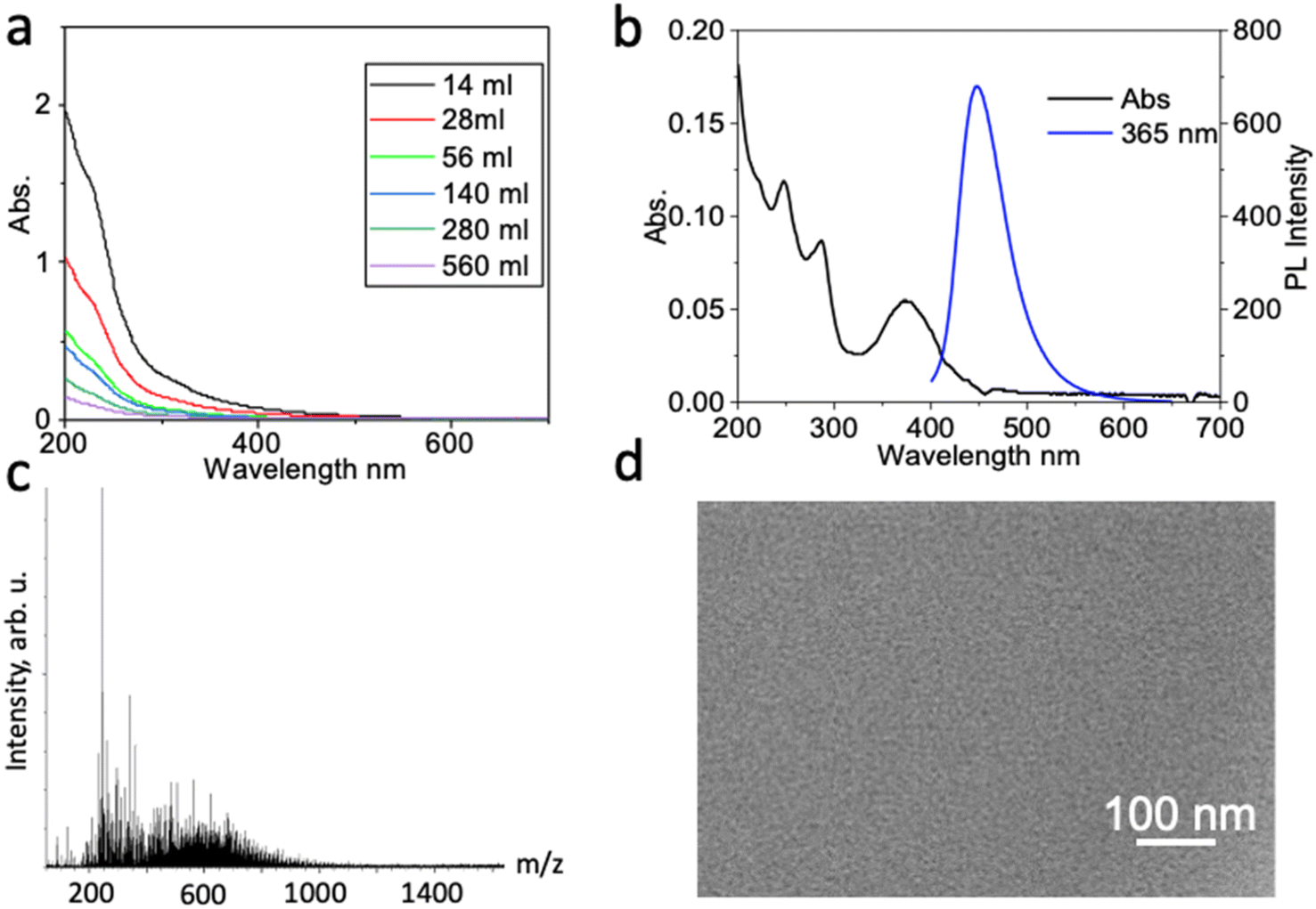Fig. 2 (a) UV-vis spectra of purified carbon dots at different solvent volumes (concentrations). The carbon dots are synthesized according to the 3rd batch of carbon dots in ref. 65. Accurate absorbances were extracted using the Beer–Lambert law. (b and c) The problem of spurious fluorescence can even affect high-yield carbon dot syntheses: (b) UV-vis absorption (black) and fluorescence (blue, excited at 365 nm) spectra taken from a product where we replicated the ‘b-GQD’ blue-fluorescent graphene quantum dot synthesis and purification protocol from ref. 66. (c) Mass spectrometry of the fluorescent product reveals that the fluorescence-active material in the product mixture consists of small molecules with molecular mass under 1000 Da. (d) TEM image of the fluorescent-active material reveals that no nano-sized carbon dots can be found in the fluorescent fraction.

When sharp features are seen in an absorption spectrum, it generally reflects vibronic sub-bands of small-molecule impurities, for example the red-fluorescent fraction in Fig. 1d of ref. 12 or the black trace in Fig. 2b shown here. In particular, we have investigated a number of fluorescent carbon dot fractions from different precursors treated by solvothermal synthesis or top-down synthesis, and found that the fluorescence is often associated with small molecules; a good example is the ‘red’ carbon dots discussed in ref. 35, whose actual fluorophore phenazine was identified in ref. 14. Fig. 2b–d shows another example from a different type of synthesis: MS reveals the presence of small molecules in the purified product, and TEM shows no significant fraction of carbon dots in the fluorescent product. The synthesis does produce carbon dots, but the fluorescence comes from small molecule impurities not sufficiently removed by the dialysis and silica gel chromatography purification protocol. Thus great care should be taken when exciting structured regions of carbon dot absorption to probe emission, making sure that the feature in the absorbance results from a moiety attached to the dot, not from a freely diffusing small molecule.⁸

Carbon dots have a wide range of bulk quantum yields, with the highest reliable measurements (i.e. not due to small molecule byproducts) generally around 10 to 50%.⁷⁶ When absorber (core of the dot) and emitter (surface groups) are separated, for example the blue to green dots in ref. 77, fluorescence can be size-independent.⁷⁸ Energy transfer from the core to the surface occurs in picoseconds, populating fluorescent surface states.⁵⁰ Internal conversion or intersystem crossing lower the quantum yield of carbon dots, and this aspect represents an area where single particle studies can provide much assistance. Surface oxidation can increase the quantum yield of carbon dots,⁷⁹ and other modifications such as PEGylation of carboxylates on the surface have also been reported to increase quantum yield,⁸⁰ although we have found rather modest changes when we reproduced such experiments.

In summary for Section 2.4, to conclusively verify the absence of small molecular byproducts, a comprehensive analytical approach is necessary. ¹H NMR should be cross-checked with a combination of additional techniques such as Mass Spectrometry in both the low (<1 kDa) and high (>30 kDa) range, High-Performance Liquid Chromatography (HPLC), and complementary NMR methods such as ¹³C NMR, DOSY-NMR to ensure thorough purification.^37,62,81 Sharp features in highly sensitive UV-vis absorption spectra, often indicative of small molecule vibronic progressions, should be viewed with caution, and there change of intensity with respect to broad background absorption after a purification step indicates continued presence of small molecules. In such a case, single particle spectroscopy such as measurements of the diffusion constant can identify even very low concentrations of small molecule contaminants.⁸ We thus turn to single-particle measurements next.

3 Carbon dots: single-particle properties

3.1 Photon-based probe techniques

While single molecule spectroscopy is more powerful than bulk measurements for heterogeneous nanomaterials like carbon dots, bulk absorption, fluorescence, and quantum yield measurements nonetheless form an important basis for further characterization, as long as they can be carried out on purified samples free of small molecules and oligomers, as discussed in the previous section. In addition to improving quantum yields, the origin of the carbon dot emission and its wavelength tunability have received considerable attention,⁵² as understanding the emission mechanism would allow for rational color tuning and optimized yields. While different mechanisms have been suggested based on single particle spectroscopy,^{17,50,82–84} with the majority involving radiative recombination of charges localized in surface states, a comprehensive molecular level picture is still missing due to the difficulty of correlating chemical structure to optical properties, as also further elaborated below in our discussion on modeling carbon dots. Nevertheless, especially single carbon dot emission spectroscopy has been able to at least partially resolve some of the unusual trends observed by bulk fluorescence spectroscopy, such as the excitation wavelength dependence of the carbon dot emission spectra.^17,38,85

For bulk spectra the emission maximum redshifts as the excitation wavelength is increased, implying that either the ensemble carbon dot solution is comprised of a collection of dots that can be photo-excited selectively and as a sum then add up to the ensemble spectrum, or that each carbon dot itself supports several chromophores with varying excitation energies, as well as of course a combination of these two possibilities. Early work that resolved single carbon dot spectra found that the spectra recorded at room temperature are narrower compared to the bulk spectrum and have maxima that are randomly shifted, covering the range of the ensemble results (Fig. 3a). These carbon dots were produced by microwave synthesis from sucrose and PEG. From the single particle spectra, it was furthermore possible to resolve a lower energy shoulder with an energy separation of 70 to 150 meV with respect to the main emission peak. This lower energy band was assigned to the excitation of optical phonons coupled to radiative charge carrier recombination; a detail otherwise hidden within the broad ensemble spectrum. This work therefore concludes that the ensemble heterogeneity and resulting excitation wavelength dependence originates from inter-dot variations, as further illustrated by exciting the same dot with both 467 and 488 nm (Fig. 3b). In fact, it is argued that these carbon dots consist of only one chromophore that is excited and likely the same one emits again based on excitation and emission polarization measurements that resolved individual and importantly parallel absorption and emission dipoles, which are fixed and do not re-orient based on repeated imaging.

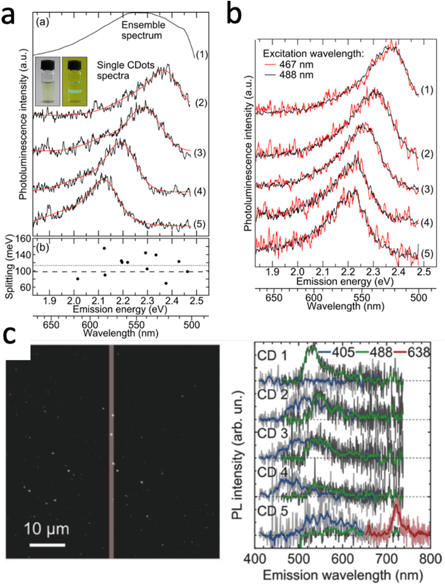Fig. 3 (a) Ensemble emission spectrum of carbon dots in water (1) and single particle photoluminescence spectra of four carbon dots on glass (2–5). The inset is a photograph of the ensemble solution excited with 488 nm seen through a long-pass filter. Also given are the separations between zero-phonon and phonon-assisted emission bands. (b) Single particle emission spectra of five carbon dots on glass. A 20 MHz white light laser system with tunable filters excited the same dots with wavelengths of 467 nm (red) and 488 nm (black) individual carbon dots did not show an excitation wavelength dependence suggesting that sub-ensembles of carbon dots with one chromophore are responsible for excitation-dependent emission seen in ensemble spectra.¹⁷ (c) Single particle emission spectra of five carbon dots taken on a homebuilt widefield fluorescence microscope. Emission image (left) visualizing the spectra (right) taken from the particles within the ∼1 μm slit of the spectrometer. Excitation with 405 nm (blue), 488 nm (green), and 638 nm (red) continuous wave lasers reveal an excitation-wavelength dependence of the emission for individual carbon dots.⁸²

Although it appears generally accepted that inter-dot heterogeneity contributes to the ensemble emission spectrum and can explain the excitation wavelength dependence, a more recent study provides evidence that each carbon dot itself can support multiple chromophores that are selectively excited with different wavelengths.⁸² Using a broader range of excitation wavelengths, single carbon dots prepared under refluxing of chloroform and diethyl amine were measured successively with 638, 488, and 405 nm laser light. While blue emission with 405 nm excitation was seen for all of the five carbon dots in Fig. 4c, the majority of dots also displayed green emission with 488 nm excitation, while one supported distinct blue, green, and red emission for all three excitation wavelengths. Importantly, adding up many single dot emission spectra measured for these three excitation wavelengths separately reproduced well the excitation wavelength dependent bulk fluorescence spectra. Hence, dot-to-dot emission peak dispersion as well as individual dots supporting multiple and different chromophores can play a role.

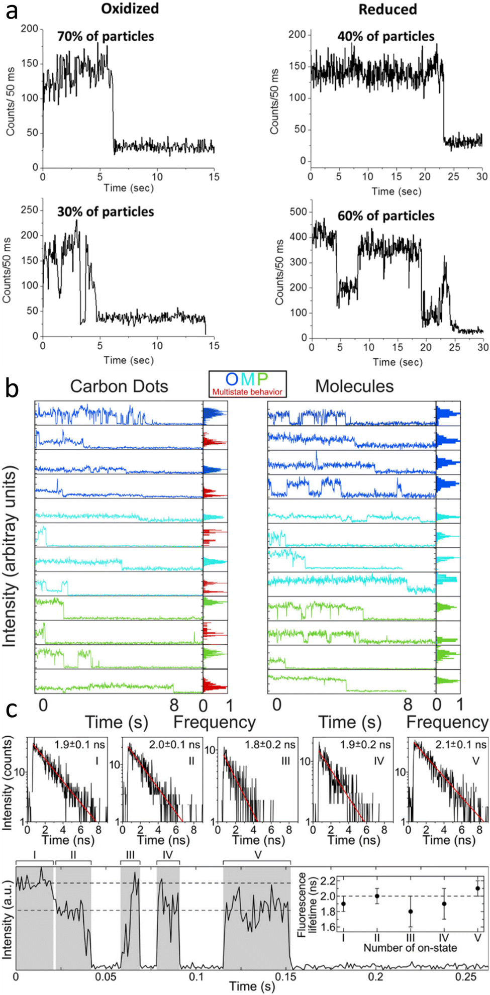Fig. 4 (a) Single carbon dot emission intensity trajectories excited with 561 nm for oxidized (left) and reduced (right) carbon dots, showing examples of carbon dots with only one (top) vs. multiple (bottom) intensity levels before single-step bleaching. Electrochemical reduction fills trap states, increasing the number of emitters and total emission counts.⁸³ (b) Single particle fluorescence intensity trajectories of synthesized carbon dots and small molecules found in the carbon dot solution. The left panel displays trajectories for carbon dots made from three different precursors distinguished by the blue, teal, and green data. The right column contains the data for the small molecules found in the corresponding carbon dot solution. On the right side of each panel is an intensity histogram, further illustrating that the carbon dots exhibit multistate state behavior (red) with single-step bleaching while the molecules only show one intensity before turning off.¹⁴ (c) Single particle fluorescence intensity trajectory with several fluorescence lifetime resolved blinks and single-step bleaching. The bottom panel contains the trajectory with each emission event labeled by numerals. The fluorescence lifetime shown in the panel above was extracted from the decay associated with each event. The average lifetime from each of the five events in the trace is 2.0 ns and implies that throughout the trace the emitting moiety remained the same despite the change in total intensity.⁸⁴

It is important to highlight that despite the differences seen in these two studies, the number of different chromophores is small. Thus, isolating the chemical nature of the emitting centers at the single dot level could therefore tremendously accelerate our understanding of their optical properties, especially when coupled with high throughput measurements and theoretical modeling, as mentioned further below.

There are also some studies claiming the absence of any heterogeneity between single particle spectra as well as in comparison to the ensemble spectrum, potentially because their preparation strategies either produced homogeneous molecular aggregates of chromophores, or predominantly emission from individual molecular precursors. In ref. 82 and 83 in particular, which uses benzene-1,2-diamine as a precursor, the spectra attributed to carbon dots actually match the small molecule phenazine, explaining the complete absence of heterogeneity.

Finally, it should be noted that in the few studies recording single carbon dot emission spectra, no evidence for spectral diffusion has been given so that it is not clear from the analysis of spectra if for carbon dots supporting multiple emissive sites energy transfer between them is possible. Likely low temperature emission spectroscopy is needed to understand if spectral diffusion indeed occurs in carbon dots. A technically easier approach to understand the existence and coupling of multiple emitters on the single dot level is to record emission transients to characterize blinking and bleaching, both hallmark attributes of single-molecule and single-particle spectroscopy.^86–89

For single molecules, emission blinking and bleaching refer to the intermittent and permanent decrease of the intensity to the background level, respectively,^86,87 often observed in a digital on-off behavior for the former. Bleaching occurs due to irreversible photochemistry that renders the fluorophore non-emissive, while blinking for single molecules typically involves the transient population of a dark state such as a spin triplet that non-radiatively returns to the ground state, thereby enabling the recovery of the bright singlet state. Although based on slightly different mechanisms, blinking and especially single-step bleaching has also been observed for a variety of inorganic and organic nanomaterials, like semiconductor quantum dots,^88,89 conjugated polymers,⁹⁰ and carbon dots.^83,84,91 For single chromophoric systems, single-step photo-bleaching as a sudden permanent intensity turn off appears trivial, but yet represents a tremendously important proof that indeed a single object, and not an aggregate, is measured. For multi-chromophoric systems such as multiple uncorrelated dye labels,⁹² discrete intensity jumps corresponding to individual bleaching events can be used to count the number of emissive units. However, a concerted photobleaching even for many chromophores has surprisingly been observed for systems like conjugated polymers,⁹⁰ where the excitation energy is often funneled into one bright chromophore that eventually undergoes single-step photo-bleaching turning the entire nanomaterial dark, i.e. a photogenerated dark state quenches all chromophores.

Indeed, single-step photobleaching has also been reported for the majority of single carbon dot studies, regardless of evidence for single emitting sites or multi-chromophoric systems. The latter explanation was invoked based on the fluorescence transients recorded for oxidized and reduced carbon dots that were prepared from nanodiamond powders.⁸³ Oxidized carbon dots mainly displayed one emission intensity level, while the reduced carbon dots primarily showed multi-level behavior (Fig. 4a). However, for all carbon dots in oxidized and reduced forms both trends were seen, as indicated by the percentages in Fig. 4a. It was suggested that the increase in multi-level emission and with it an overall increase in total photon counts is related to the electrochemical reduction of the carbon dots, filling trap states and hence reducing non-radiative pathways.

Our recent single-particle fluorescence imaging of carbon dots in comparison to their molecular precursors also revealed more complex, multi-level emission transients, indicative of multiple, albeit few chromophores for some dots, while the single molecular precursors displayed the expected one intensity level blinking and bleaching behavior (Fig. 4b). The assignment of multiple intensity levels to multiple chromophores coupled with single-step photo-bleaching implies that these chromophores must be electronically coupled. More work is needed though to decipher the underlying energy and charge transfer processes.

A different interpretation for multiple emission intensity levels has emerged by a study that correlated emission intensities with lifetimes. Carbon dots synthesized from urea and p-phenylenediamine by a hydrothermal method displayed at least two levels with distinct emission intensities. However, their mono-exponential lifetimes were always similar for the same dots (Fig. 4c), implying that the emissive site was the same. The lower intensity level was therefore assigned to a gray state based on the following mechanism that was developed also from the observed power law behavior of emission on and off times. Quenching by Dexter-type electron transfer to surface groups modulates the emission intensity between bright, gray, and off states, while electron transfer from the core to the surface restores the bright on state. It was further argued that only one surface chromophore with a fixed orientation exists per dot and that it is excited directly, as obtained from polarization sensitive imaging.

Regardless of the photo-blinking mechanism, its presence has allowed for the application of carbon dots in super-resolution imaging. Taking advantage of their stochastic blinking, one can super-localize individual carbon dots to a few tens of nanometers by point spread function fitting even for densely labeled biological systems as not all carbon dots are bright at the same time. Furthermore, photoactivation with a 401 nm laser was demonstrated after exciting carbon dots with a 639 nm laser, which causes emission but also produces a dark cationic state that is recovered with blue light. This dynamic behavior is ideal for implementing photo-activation strategies that have been developed for super-resolution imaging techniques.

In summary, single-particle optical emission spectroscopy presents a powerful approach to remove or at least reduce the heterogeneity intrinsic to bottom-up synthesis of carbon dots and therefore allows underlying mechanisms to be established. In addition to heterogeneity within the same sample batch, one should also ask about reproducibility of not only synthesis methods, but also optical properties determined by single-particle methods for carbon dots prepared by accepted, common processes. Unfortunately, there have not been enough single-particle emission studies reported to compare results for similarly prepared carbon dots. Specifically, for the results highlighted in Fig. 3 and 4, the carbon dots were synthesized from sucrose and polyethylene glycol in a microwave,¹⁷ refluxing of chloroform and diethylamine,⁸² high temperature annealing of nanodiamond powders in a furnace,⁸³ and by combining urea and 0.2 g of p-phenylenediamine in an autoclave.⁸⁴ These vastly different synthesis methods, likely resulting in carbon dots with quite different chemical compositions and structures, explain why dissimilar and even contradicting optical studies have been reported (Fig. 3 and 4), even if common features like photo-blinking has been observed in the majority of studies. More work is therefore needed to test reproducibility among several labs for carbon dots made by one or a few standard and agreed-upon methods. We further note that this issue has also been encountered in other areas of nanoscience and it took improvements in both synthesis and characterization to establish best protocols as well as reproducible optical, magnetic, and electronic properties that then can be accurately modeled.

3.2 Electron-based probe techniques

To verify the dimensions and shape of carbon dots, single particle transmission electron microscopy has proved invaluable. Although observation of nanoparticles by TEM does not guarantee that bulk optical properties of a sample originate from such particles made in low yield, it is important as a gold standard to verify that nanoparticles are at least present, and surprisingly often neglected in the carbon dot literature. While a layered crystalline structure is frequently observed for top-down dots, bottom-up syntheses yield more amorphous products. Nonetheless, regular lattice spacings have been observed, for example in urea/phenylenediamine-based carbon dots made by hydrothermal synthesis where a 0.21 nm lattice spacing characteristic of (100) graphene layering was observed.⁷⁷ As discussed in Section 2, TEM is an excellent tool for size-distribution characterization. While top-down crystalline carbon dots can have sharply peaked (as low as ±3%) size distributions, bottom-up carbon dots also often have narrow size distributions (±10%), e.g. o-carbon dots in ref. 14. This distribution is not as narrow as for quantum dots, but still suggests that homogeneous nucleation and capping by oxidation (heteroatoms localized on the outer shell of carbon dots) controls the size of carbon dots in solvothermal synthesis.⁹³

Single particle AFM and STM measurements also provide valuable information on shape and electronic structure of carbon dots. In particular, high resolution AFM in tapping mode, which relies on Pauli exclusion (degeneracy pressure) to measure repulsive walls of intermolecular electronic potentials, has revealed highly structured carbon dot aggregation on surfaces, producing either rod-like or ring-like oligomers.⁹⁴ Individual carbon dots in the aggregates can be made out when ∼10 nm diameter dots were synthesized. While AFM, unlike TEM, cannot be used to reliably determine particle diameters, it is complementary to TEM because it can be used to estimate particle heights. Thus, tapping mode AFM has shown that some bottom-up-syntheses indeed produce multi-layered particles in the 2–4 nm height range, as opposed to graphene-like single-layer discs.⁹⁵

Scanning tunneling microscopy current–voltage (I–V) curves in particular reveal that bandgaps are inhomogeneously distributed over carbon dots.¹² In dots derived from benzene tetracarboxylic acid and diaminofluorene,¹² bandgaps measured by STM over the bulk lie in the 5 eV range (UV absorption), whereas at isolated surface sites bandgaps in the 1.8 to 2.1 eV (red to blue fluorescent surface sites) are observed (Fig. 5a and b). This evidence supports the idea that the bulk of the carbon dot has a bandgap in the UV region, whereas surface-modified sites can have smaller bandgaps that lead to visible fluorescence. pH sensitivity shows that the dots contain phenolic or carboxylate groups at the surface. It is worth noting that the reddest-fluorescing fraction of these carbon dots purified using chromatography contains a sharp absorption band probably due to a small molecule.

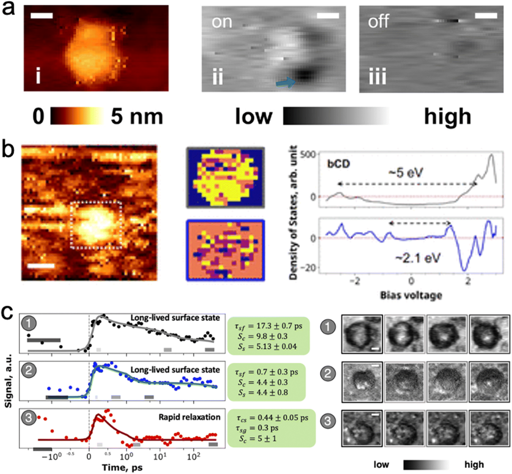Fig. 5 Carbon dot emission is a core – defect interaction. (a) STM image of optical defect excitation: (i) STM topography; (ii) SMA-STM reveals a localized excited defect with laser excitation; (iii) the defect is not visible without laser excitation. (b) STM position-resolved I–V curves determine that there are two main spatial components (yellow in the middle figures) in the optical transition: a core transition with a bandgap of 5 eV that encompasses the whole carbon dot; and surface defect sites with a smaller bandgap of ≈2.1 eV.¹² (c) Time-resolved SMA-STM resolves the picosecond lifetime of the optically excited defect. Carbon dots (1) and (2) settle into a long lived (>200 ps) excited state, whereas dot (3) swiftly decays back to the ground state. The longer-lived excited states have the opportunity to fluoresce with high quantum yield, whereas the dots with short excited-state lifetime reduce the average quantum yield of the bulk sample⁵⁰ Adapted with permission from ref. 12 (panels (a) and (b)) and 50 (panel (c)).

SMA-STM (single molecule absorption STM) experiments, in which the nanoparticle under the STM tip is excited by a laser, and the tip probes how the tunneling current is modulated by nanoparticle electrons that occupy excited state orbitals, also shows that there are localized surface excitations on some carbon dots. For blue benzene tetra-acetic acid/ethylenediamine-derived dots, SMA-STM reveals that localized electronic density on the dots corresponds to bandgaps of about 2.6 eV, closely aligned with the 477 nm observed fluorescence.¹² Time-resolved SMA-STM (Fig. 5c), in which a femtosecond pump-probe laser pulse sequence excites and then depletes an excited state orbital, thus modulating tunneling current through the carbon dot into the substrate, demonstrated that absorbed energy is transferred form the core to localized (<1 nm) surface states in a few picoseconds.⁵⁰ Two types of surface states were found: ones with a >200 ps lifetime, and ones with a <10 ps lifetime. This result suggests that the bulk quantum yield observed for such carbon dots could come from a mixture of very high quantum yield dots with long-lived surface states that fluoresce, and very low quantum yield dots with surface states that decay via nonradiative processes such as internal conversion from the excited surface electronic state back down to the vibrationally excited ground state (see next section on electronic structure calculations).

Despite the power of single dot imaging and spectroscopy to provide detailed insights into their structure as well as their electronic and optical properties, two main challenges exist going forward in order to relate observables with theory and mechanistic models: first, the higher complexity of single particle measurements compared to standard ensemble measurements typically implies that for a particular sample only one or a few observables are recorded on an already challenging setup, such as, for example, radiative properties only deduced from emission microscopy vs. electronic bandgaps and absorption by SMA-STM. This point is evident from the limited number of single dot studies performed to date. Ideally, highly multi-modal acquisition should be developed to record simultaneously several observables that are intimately linked and needed to acquire a comprehensive picture of the photophysics and photochemistry of carbon dots, especially as this knowledge can in turn be used to optimize carbon dot synthesis. In particular, closely linking absorption with emission for the same single carbon dot promises to yield tremendous new insights with respect to unwanted non-radiative relaxation pathways as well as the possibility to directly determine absolute emission quantum yields on a single dot level. In fact, a clever ensemble cavity spectroscopy approach that quantifies yields through the distance dependent modulation of the radiative lifetime has shown that the bulk emission quantum yield obtained by comparison to standards underestimates the true quantum yield of graphene dots due to the presence of non-emissive dots.⁹⁶ Another challenge is to directly and continuously connect the ultrafast transient absorption dynamics on the picoseconds timescale with the slower emission lifetimes occurring over several nanoseconds.

Second, in conjunction with multi-modal imaging it is imperative that data throughput is drastically increased to establish the behavior of hundreds to thousands of carbon dots and potentially even more so that patterns can be identified together with outliers that can prove to be equally important for the understanding and optimization of carbon dots. Multi-modal instruments must therefore be automated to run independent of slow user input and ideally even incorporate in situ analysis that forms the feedback for measurement control, establishing in an autonomous way when enough dots, large enough signal-to-noise, or a sufficiently long transients have been acquired. Machine learning methods to control such smart microscopes are undoubtedly a major asset as long as their analysis algorithms remain grounded in physical models. The challenge of automation is not unique to carbon dots. However, given the diversity in synthesis procedures and the still unknown structures together with the multitude of possible chemical surface groups, high throughput is clearly needed to investigate different carbon dot samples in various environments (e.g., pH) or oxidation states. Tackling this large sample parameter space on the single dot level will only be possible through clever measurement automation, which needs to occur together with the speedy analysis of large data sets as well as theoretical modeling, a topic that is reviewed next.

4 Carbon dots: electronic structure

Given the two-fold capabilities to adjust synthetic methods to tune carbon dot properties and to make spatially-resolved spectroscopic observations of the resulting dynamics, the ability to directly map atomistic structure to function feels tantalizingly close. Electronic structure simulations can provide an important missing link. Simulation studies to date paint a complex picture of the electronic structure of carbon dots, in which their properties arise from networks of chromophores that exchange energy and charge via numerous pathways.^97–103 Yet carbon dots push standard simulations tools to their limits, given that bottom-up carbon dot materials can only be described in terms of large ensembles of disordered structures. These limitations are driving the development of new computational tools that work hand-in-hand with experiment to define and explore large ensembles of carbon dot structures for comparison with experiments.

For nanoscale systems like carbon dots, density functional theory (DFT) and its excited state extension, time-dependent density functional theory (TDDFT), remain the primary workhorse electronic structure methods, owing to the balance between accuracy and computational cost that they provide. A DFT calculation takes as input a precise molecular structure and provides as output a prediction of any of a number of molecular properties—total energy, optimized molecular structure, electronic density of states, etc. TDDFT can go a step further and provide information about electronic excitations, e.g. absorption/emission energies and oscillator strengths. In a sense, a single DFT calculation is similar to a single particle experiment. They both provide the properties of a single unique structure, drawn from the ensemble of possible structures. However, unlike in the experimental case, in the context of a DFT calculation the precise atomistic structure is known and may be chosen by the scientist.

One may therefore design their own computational experiments, by varying the atomistic structure in thoughtful, well-controlled ways and observing the resulting change in properties. For example, as can be seen in Fig. 6a, simulations of idealized carbon dot structures with highly conjugated sp² cores have indicated the existence of quantum confinement effects, akin to those observe in inorganic quantum dots.¹⁰⁴ In dots with mixed sp²/sp³ character, it is the size of the sp² domains that determine the excitations energies.^104,108,109 Computational experiments on small single-layer dots indicate that graphitic N defects significantly shift the lowest absorption bands of carbon dots (Fig. 6b),^105,110 and that surface functional groups can impact the luminescence via charge transfer to/from the sp² core.^101,111,112 A thorough overview of specific heteroatom effects can be found in the nice perspective article by Yu, et al.¹⁸

Fig. 6 Understanding structure–function relationships using computational experiments. (a) Quantum size effects determine emission wavelength of ideal sp² carbon dots.¹⁰⁴ (b) The existence and position of heteroatom defects directly impact the lowest absorption band.¹⁰⁵ (c) Heteroatoms also distort structure, resulting in the localization of excitations.¹⁰⁶ (d) Different arrangements of chromophores in more realistic carbon dots (in this case π stacked) determine relaxation pathways.¹⁰⁷

Density functional calculations also allow us to approximate and observe the electronic wave function itself, providing information that is not observable experimentally.¹¹³ Where single particle luminescence measurements provide information about the transition dipoles and SMA-STM experiments can provide nanoscale spatially resolved information about electronic excitations, simulation provides a picture of the electronic excitations on sub-atomic length scales. For example, even in relatively ideal dots, heteroatom defects both at the surface and in the core can indirectly cause the excitations to localize by breaking the planarity of the system (Fig. 6c).^106,108 Calculations of realistic carbon dots comprised of multiple conjugated subunits demonstrate that nearly any conceivable contact between conjugated units (covalent, stacked, hydrogen bonded, etc.) can introduce electronic coupling (Fig. 6d).^107,114

The picture of the electronic structure of carbon dots that arises from these theoretical studies and the single particle experiments described above is quite complex. In the rare case of a perfect sp²-conjugated layer, excitons may be delocalized over the entire dot. But in the more realistic case, the disordered and defective atomistic structures of bottom-up carbon dots will have excitations that are localized to smaller chromophores. Each such unit is electronically coupled to its neighbors through covalent linkers (conjugated or not), hydrogen bonds, π-stacking, or other intermolecular interactions, introducing a complex three-dimensional network of energy and charge transfer pathways. It is these pathways that control the exciton dynamics, and the ultimate fate of an electronic excitation: does it decay radiatively or nonradiatively? If radiatively, at what wavelength and which lifetime? And the answers to these questions may not be static. Weak intermolecular interactions allow both thermal and photochemical rearrangements, which may dynamically modify the energy landscape so as to favor one pathway over another.¹¹⁵ Additionally, one must consider that the ensemble of experimentally realizable carbon dots is vast. Each carbon dot is likely to be unique, like a snowflake, with its own set of energy transfer pathways. It is only by averaging over a massive ensemble of such structures that the macroscopic behavior may be understood. In fact, considering an ensemble of carbon dot structures differing only in the fraction of sp² hybridized carbons, Kundelev et al. account for two of the more idiosyncratic features of experimentally observed carbon dot luminescence: large Stokes shift and strong excitation wavelength dependence (Fig. 7a).¹⁰⁹

Fig. 7 Understanding the underlying ensemble. (a) The PL excitation wavelength dependence can be explained in terms of the variable degree of sp² hybridization within an ensemble of carbon dots.¹⁰⁹ (b) Excitation wavelength dependence of two samples of stoichiometrically identical carbon dots.¹⁴ (c) Interior N defects result in weak quantum size effects in ensembles of o- and p-carbon dots compared to m-carbon dots.¹⁴

Considering this picture, it is clear that the close connection between atomistic structure and function is both the great strength and the most limiting feature of DFT-based computational experiments. DFT is well suited for designing experiments based on minor variations of an ideal system. But on its own, DFT does not compute ensemble properties unless it is fed an ensemble of structures and a proportionally large allotment of computer resources. Without the ability to investigate ensemble properties, we are limited in the questions we can ask and in the connections we can draw between simulation and experiment.

In plotting a path forward, we must ask how we can determine an experimentally realistic ensemble of possible structures for subsequent analysis. It might be tempting to use simulation to determine realistic structures, but with current technology, this is impossible. DFT is extremely useful for predicting the thermodynamic properties of materials. For example, it is widely used to predict the presence and stability of defects in crystalline materials,¹¹⁶ and it has been used to great effect to explore the structural ensembles of heterogeneous catalysts.¹¹⁷ But carbon dots have less in common with relatively labile inorganic materials than with organic molecules. As in a typical organic synthesis, the goal of carbon dot synthesis is not to achieve thermodynamic equilibrium, but rather to kinetically trap a thermodynamically unstable arrangement of atoms with desirable properties. Structural determination by direct simulation of the synthetic process, which may last several hours and involve an astronomically large network of chemical reactions, is not presently feasible. Thus, the path to determining the structural ensemble cannot rely on theory alone, and instead must incorporate experimental data and/or knowledge of the synthetic procedure.

We have recently used experimental hints at the structural ensemble to elucidate surprising differences between the luminescence observed from carbon dots synthesized under similar conditions from three precursors: ortho-, meta-, and para-diaminobenzene. Obviously, if these three stoichiometrically identical systems were brought to equilibrium, the resulting carbon dots would have identical structural ensembles and properties. However, dramatic differences in the luminescence are observed. Carbon dots synthesized from m-diamino benzene (m-carbon dots) exhibit strong excitation wavelength dependence, where o- and p-carbon dots exhibit almost no dependence (Fig. 7b right and left, respectively).¹⁴ This behavior suggests that m-carbon dots include a much wider variety of emitting states than o- and p-carbon dots. Having observed the presence of a few small-molecule intermediates (different phenazine diamines for o- and p-carbon dots and 2-methylquinolin-7-amine for m-carbon dots), we generated small ensembles of larger o-, m-, and p-carbon dot structures constructed from the appropriate precursor units. Fig. 7c indicates that computed o- and p-carbon dots' luminescence wavelengths are very insensitive to particle size, whereas those for m-carbon dots exhibit more typical quantum size effects. Analysis of the electronic structure indicates that graphitic N defects in o- and p-carbon dots break the conjugation, resulting in very localized excitons with size-insensitive emission. In contrast, N defects in m-carbon dots tend to be on the edges of the flakes, allowing for delocalized core excitations with size-sensitive emission.

In this case, we took a synthesis-centered approach and chemical intuition to generate a small structural ensemble. But ideally tools would exist to take advantage of all available experimental information. A natural path forward would be to use multi-experimental datasets in conjunction with artificial intelligence (AI) to generate and sample from large, unbiased structural ensembles. To date, efforts to incorporate AI into the design loop have been focused on linking synthetic parameters (e.g. precursor, solvent, temperature) to function (e.g. luminescence color and yield).^93,118–122 These studies indicate that AI provides a useful framework for predicting the properties of not-yet-synthesized carbon dots. However, these approaches focus on linking synthetic procedure directly to macroscopic properties, without consideration of the ensembles of atomistic structures underlying this relationship. Thus, they cannot provide physical understanding in the form of causal structure–function relationships, which remains the central goal of physical nanoscience.¹²³ Incorporating a representation of the structural ensemble would enable development of such physical understanding. In this sense, AI could be leveraged to enable deeper physical understanding, rather than replace it.

Once one has the tools to generate realistic structural ensembles, a second roadblock arises when one wishes to predict the properties of massive ensembles of carbon dots—many properties are difficult to compute efficiently enough to apply to an entire ensemble of structures. Computing the absorption wavelength of thousands of small (1 to 2 nm) carbon dots would be fairly routine with modern electronic structure software, but computing non-radiative rates, emission linewidths, charge/energy transfer pathways, and many other dynamical properties would not be. Thus, a deep understanding of the relationship between structural ensembles and function in carbon dots also depends on the development of highly efficient tools for simulating photophysical outcomes without explicitly computing large numbers of expensive ab initio molecular dynamics simulations. With these critical needs in mind, carbon dots offer fertile soil for ongoing computational method development efforts.

5 Outlook

Bottom-up (and top-down) carbon dots are a class of mainly carbon-based materials with several interesting optical and electronic properties. Like other organic materials, they can be less toxic to cells or tissues than quantum dots. They also can be sensitive to pH due to the surface origin of fluorescence involving (de)protonatable groups such as –COOH/–COO⁻ in many cases. Still, why pursue carbon dots for practical uses? Unlike small organic dyes, their extinction coefficients can stretch into 10⁶ M⁻¹ cm⁻¹ range, putting them among the strongest known absorbers per cross-sectional area. As single-molecule studies have shown, their larger surface is amenable to housing multiple chromophores, which can increase the resistance to total bleaching compared to single dyes. Their fluorescence properties can be independent of size, in principle allowing dots of different colors to form uniform films if size can be controlled to <5% variation. However, care must be taken particularly for bottom-up dots (much less so for top-down dots) that small molecule synthesis byproducts do not obscure the optical properties. Sharp peaks in UV-vis absorption spectra should lead the researcher to caution and use of a carefully chosen battery of NMR, mass spectroscopy, chromatography and dialysis to purify samples to the point where dot fluorescence exceeds the fluorescence of synthesis intermediates. Carbon dots are inherently heterogeneous systems with particle-to-particle differences, but modern electronic structure calculations have reached the ability to analyze such flaws. Such calculations reveal how fairly similar surface structures can lead to a wide range of fluorescence emission peaks, or how seemingly very similar precursor isomers can lead to very different dot structures and properties. Single molecule measurements have shown that some structures have very desirable properties (e.g. string absorption and near 100% quantum yield with low bleaching), but there is a large gap with bottom-up synthesis: although the latter has the promise of making chemically tailored structures even for very large molecules, we need to understand the structure–function relationship much better than we currently do to make targeted improvements in synthesis.

Data availability

This review utilized only publicly available and cited data in the literature, and where new data is given all data is included in the figures and results of the manuscript itself.

Author contributions

ZB performed experiments, did data analysis, and co-wrote the manuscript. EG performed experiments, did data analysis, and co-wrote the manuscript. MG supervised the study, did data analysis, co-wrote the manuscript, and acquired funding. BGL did data analysis, supervised research, co-wrote the manuscript, and acquired funding. SL edited the manuscript, supervised research, and acquired funding. AM carried out calculations, did data analysis, and co-wrote the manuscript. SN edited the manuscript, supervised research, and acquired funding.

Conflicts of interest

There are no conflicts of interest to declare.

Acknowledgements

ZB, EG, MG, and SL were supported by the National Science Foundation Center for Chemical Imaging (CCI) CHE 2124983. BGL and AM gratefully acknowledge support from the U.S. Department of Energy, Office of Science, Office of Basic Energy Sciences, under Award No. DE-SC0021643 and from the Institute for Advanced Computational Science. MG and SN were also funded by a research grant from KLA.

References

1. S. F. A. Acquah, A. V. Penkova, D. A. Markelov, A. S. Semisalova, B. E. Leonhardt and J. M. Magi, ECS J. Solid State Sci. Technol., 2017, 6, M3155–M3162.
2. R. Saito, G. Dresselhaus and M. S. Dresselhaus, Physical properties of carbon nanotubes, Imperial College Press, London, Repr., 2012.
3. F. Farjadian, S. Abbaspour, M. A. A. Sadatlu, S. Mirkiani, A. Ghasemi, M. Hoseini-Ghahfarokhi, N. Mozaffari, M. Karimi and M. R. Hamblin, ChemistrySelect, 2020, 5, 10200–10219.
4. J. Liu, R. Li and B. Yang, ACS Cent. Sci., 2020, 6, 2179–2195.
5. F. Bruno, A. Sciortino, G. Buscarino, M. L. Soriano, Á. Ríos, M. Cannas, F. Gelardi, F. Messina and S. Agnello, Nanomaterials, 2021, 11, 1265.
6. R. De Boëver, J. R. Town, X. Li and J. P. Claverie, Chem.–Eur. J., 2022, 28, e202200748.
7. P. Duan, B. Zhi, L. Coburn, C. L. Haynes and K. Schmidt-Rohr, Magn. Reson. Chem., 2020, 58, 1130–1138.
8. M. Righetto, F. Carraro, A. Privitera, G. Marafon, A. Moretto and C. Ferrante, J. Phys. Chem. C, 2020, 124, 22314–22320.
9. J. B. Essner, J. A. Kist, L. Polo-Parada and G. A. Baker, Chem. Mater., 2018, 30, 1878–1887.
10. Z. Li, L. Deng, I. A. Kinloch and R. J. Young, Prog. Mater. Sci., 2023, 135, 101089.
11. S. N. Baker and G. A. Baker, Angew. Chem., Int. Ed., 2010, 49, 6726–6744.
12. H. A. Nguyen, I. Srivastava, D. Pan and M. Gruebele, ACS Nano, 2020, 14, 6127–6137.
13. N. C. Verma, S. Khan and C. K. Nandi, Methods Appl. Fluoresc., 2016, 4, 044006.
14. Z. Bian, A. Wallum, A. Mehmood, E. Gomez, Z. Wang, S. Pandit, S. Nie, S. Link, B. G. Levine and M. Gruebele, ACS Nano, 2023, 17, 22788–22799.
15. V. Hinterberger, C. Damm, P. Haines, D. M. Guldi and W. Peukert, Nanoscale, 2019, 11, 8464–8474.
16. N. Gross, C. T. Kuhs, B. Ostovar, W.-Y. Chiang, K. S. Wilson, T. S. Volek, Z. M. Faitz, C. C. Carlin, J. A. Dionne, M. T. Zanni, M. Gruebele, S. T. Roberts, S. Link and C. F. Landes, J. Phys. Chem. C, 2023, 127, 14557–14586.
17. S. Ghosh, A. M. Chizhik, N. Karedla, M. O. Dekaliuk, I. Gregor, H. Schuhmann, M. Seibt, K. Bodensiek, I. A. T. Schaap, O. Schulz, A. P. Demchenko, J. Enderlein and A. I. Chizhik, Nano Lett., 2014, 14, 5656–5661.
18. J. Yu, X. Yong, Z. Tang, B. Yang and S. Lu, J. Phys. Chem. Lett., 2021, 12, 7671–7687.
19. D. Ozyurt, M. A. Kobaisi, R. K. Hocking and B. Fox, Carbon Trends, 2023, 12, 100276.
20. A. H. Loo, Z. Sofer, D. Bouša, P. Ulbrich, A. Bonanni and M. Pumera, ACS Appl. Mater. Interfaces, 2016, 8, 1951–1957.
21. H. Zhu, X. Wang, Y. Li, Z. Wang, F. Yang and X. Yang, Chem. Commun., 2009, 5118.
22. M. Otten, M. Hildebrandt, R. Kühnemuth and M. Karg, Langmuir, 2022, 38, 6148–6157.
23. C. S. Stan, C. Albu, A. Coroaba, M. Popa and D. Sutiman, J. Mater. Chem. C, 2015, 3, 789–795.
24. P. Russo, A. Hu, G. Compagnini, W. W. Duley and N. Y. Zhou, Nanoscale, 2014, 6, 2381–2389.
25. R. Liu, D. Wu, S. Liu, K. Koynov, W. Knoll and Q. Li, Angew. Chem., Int. Ed., 2009, 48, 4598–4601.
26. Y. Yang, D. Wu, S. Han, P. Hu and R. Liu, Chem. Commun., 2013, 49, 4920.
27. E. A. Stepanidenko, I. D. Skurlov, P. D. Khavlyuk, D. A. Onishchuk, A. V. Koroleva, E. V. Zhizhin, I. A. Arefina, D. A. Kurdyukov, D. A. Eurov, V. G. Golubev, A. V. Baranov, A. V. Fedorov, E. V. Ushakova and A. L. Rogach, Nanomaterials, 2022, 12, 543.
28. J. Zong, Y. Zhu, X. Yang, J. Shen and C. Li, Chem. Commun., 2011, 47, 764–766.
29. J. Deng, Q. Lu, N. Mi, H. Li, M. Liu, M. Xu, L. Tan, Q. Xie, Y. Zhang and S. Yao, Chem.–Eur. J., 2014, 20, 4993–4999.
30. H. Li, H. Ming, Y. Liu, H. Yu, X. He, H. Huang, K. Pan, Z. Kang and S.-T. Lee, New J. Chem., 2011, 35, 2666.
31. Y. Song, S. Zhu, S. Zhang, Y. Fu, L. Wang, X. Zhao and B. Yang, J. Mater. Chem. C, 2015, 3, 5976–5984.
32. D. Qu and Z. Sun, Mater. Chem. Front., 2020, 4, 400–420.
33. W. Kasprzyk, S. Bednarz, P. Żmudzki, M. Galica and D. Bogdał, RSC Adv., 2015, 5, 34795–34799.
34. M. Righetto, A. Privitera, I. Fortunati, D. Mosconi, M. Zerbetto, M. L. Curri, M. Corricelli, A. Moretto, S. Agnoli, L. Franco, R. Bozio and C. Ferrante, J. Phys. Chem. Lett., 2017, 8, 2236–2242.
35. K. Jiang, S. Sun, L. Zhang, Y. Lu, A. Wu, C. Cai and H. Lin, Angew. Chem., Int. Ed., 2015, 54, 5360–5363.
36. B. Bartolomei, A. Bogo, F. Amato, G. Ragazzon and M. Prato, Angew. Chem., Int. Ed., 2022, 61, e202200038.
37. C.-Y. Chen, Y.-H. Tsai and C.-W. Chang, New J. Chem., 2019, 43, 6153–6159.
38. Z.-H. Wen and X.-B. Yin, RSC Adv., 2016, 6, 27829–27835.
39. L. Đorđević, F. Arcudi and M. Prato, Nat. Protoc., 2019, 14, 2931–2953.
40. A. Sciortino, N. Mauro, G. Buscarino, L. Sciortino, R. Popescu, R. Schneider, G. Giammona, D. Gerthsen, M. Cannas and F. Messina, Chem. Mater., 2018, 30, 1695–1700.
41. L. Liu and Z. Xu, Anal. Methods, 2019, 11, 760–766.
42. X. Xu, R. Ray, Y. Gu, H. J. Ploehn, L. Gearheart, K. Raker and W. A. Scrivens, J. Am. Chem. Soc., 2004, 126, 12736–12737.
43. H. Liu, T. Ye and C. Mao, Angew. Chem., Int. Ed., 2007, 46, 6473–6475.
44. Y. Yan, L. Xia and L. Ma, RSC Adv., 2019, 9, 24057–24065.
45. Y. Dong, H. Pang, H. B. Yang, C. Guo, J. Shao, Y. Chi, C. M. Li and T. Yu, Angew. Chem., Int. Ed., 2013, 52, 7800–7804.
46. A. B. Siddique, A. K. Pramanick, S. Chatterjee and M. Ray, Sci. Rep., 2018, 8, 9770.
47. Y. Xu, M. Wu, Y. Liu, X. Feng, X. Yin, X. He and Y. Zhang, Chem.–Eur. J., 2013, 19, 2276–2283.
48. S.-L. Hu, K.-Y. Niu, J. Sun, J. Yang, N.-Q. Zhao and X.-W. Du, J. Mater. Chem., 2009, 19, 484–488.
49. S. Khan, A. Sharma, S. Ghoshal, S. Jain, M. K. Hazra and C. K. Nandi, Chem. Sci., 2018, 9, 175–180.
50. H. A. Nguyen, I. Srivastava, D. Pan and M. Gruebele, Proc. Natl. Acad. Sci. U.S.A., 2021, 118, e2023083118.
51. Q. Xu, Q. Zhou, Z. Hua, Q. Xue, C. Zhang, X. Wang, D. Pan and M. Xiao, ACS Nano, 2013, 7, 10654–10661.
52. A. P. Demchenko and M. O. Dekaliuk, Nanoscale, 2016, 8, 14057–14069.
53. A. L. Himaja, P. S. Karthik and S. P. Singh, Chem. Rec., 2015, 15, 595–615.
54. S. Thambiraj and D. R. Shankaran, Appl. Surf. Sci., 2016, 390, 435–443.
55. K. Bankoti, A. P. Rameshbabu, S. Datta, B. Das, A. Mitra and S. Dhara, J. Mater. Chem. B, 2017, 5, 6579–6592.
56. W.-J. Wang, J.-M. Xia, J. Feng, M.-Q. He, M.-L. Chen and J.-H. Wang, J. Mater. Chem. B, 2016, 4, 7130–7137.
57. K. J. Mintz, M. Bartoli, M. Rovere, Y. Zhou, S. D. Hettiarachchi, S. Paudyal, J. Chen, J. B. Domena, P. Y. Liyanage, R. Sampson, D. Khadka, R. R. Pandey, S. Huang, C. C. Chusuei, A. Tagliaferro and R. M. Leblanc, Carbon, 2021, 173, 433–447.
58. A. Philippidis, A. Spyros, D. Anglos, A. B. Bourlinos, R. Zbořil and E. P. Giannelis, J. Nanopart. Res., 2013, 15, 1777.
59. H. Tang, Y. Tang, M. Xiao, H. Zhu and M. Guo, Colloids Surf., A, 2022, 651, 129564.
60. R. Evans, G. Dal Poggetto, M. Nilsson and G. A. Morris, Anal. Chem., 2018, 90, 3987–3994.
61. D. A. Sousa, M. N. Berberan-Santos and J. V. Prata, Chem.–Eur. J., 2024, 30, e202302955.
62. F. Wang, Z. Xie, H. Zhang, C. Liu and Y. Zhang, Adv. Funct. Mater., 2011, 21, 1027–1031.
63. V. Ţucureanu, A. Matei and A. M. Avram, Crit. Rev. Anal. Chem., 2016, 46, 502–520.
64. E. Dervishi, Z. Ji, H. Htoon, M. Sykora and S. K. Doorn, Nanoscale, 2019, 11, 16571–16581.
65. S. Zhu, J. Zhang, X. Liu, B. Li, X. Wang, S. Tang, Q. Meng, Y. Li, C. Shi, R. Hu and B. Yang, RSC Adv., 2012, 2, 2717.
66. L. Wang, Y. Wang, T. Xu, H. Liao, C. Yao, Y. Liu, Z. Li, Z. Chen, D. Pan, L. Sun and M. Wu, Nat. Commun., 2014, 5, 5357.
67. B. Zhang, B. Wang, G. Xing, Z. Tang and S. Qu, Chin. Chem. Lett., 2024, 35, 109358.
68. T. N. Nguyen, P. A. Le and V. B. T. Phung, Biomass Convers. Biorefin., 2022, 12, 2407–2416.
69. X. Jia, J. Li and E. Wang, Nanoscale, 2012, 4, 5572.
70. D. Das and R. K. Dutta, ACS Appl. Nano Mater., 2021, 4, 3444–3454.
71. J. Hou, J. Li, J. Sun, S. Ai and M. Wang, RSC Adv., 2014, 4, 37342.
72. H. Song, X. Liu, B. Wang, Z. Tang and S. Lu, Sci. Bull., 2019, 64, 1788–1794.
73. M. Vedamalai, A. P. Periasamy, C.-W. Wang, Y.-T. Tseng, L.-C. Ho, C.-C. Shih and H.-T. Chang, Nanoscale, 2014, 6, 13119–13125.
74. F. Meng, H. Xu, S. Wang, J. Wei, W. Zhou, Q. Wang, P. Li, F. Kong and Y. Zhang, RSC Adv., 2022, 12, 19686–19694.
75. Q. Zhang, R. Wang, B. Feng, X. Zhong and K. Ostrikov, Nat. Comm., 2021, 12, 6856.
76. W. Fawaz, J. Hasian and I. Alghoraibi, Sci. Rep., 2023, 13, 18641.
77. H. Ding, S.-B. Yu, J.-S. Wei and H.-M. Xiong, ACS Nano, 2016, 10, 484–491.
78. S. Hu, A. Trinchi, P. Atkin and I. Cole, Angew. Chem., Int. Ed., 2015, 54, 2970–2974.
79. I. Srivastava, S. K. Misra, I. Tripathi, A. Schwartz-Duval and D. Pan, Adv. Biosyst., 2018, 2, 1800009.
80. H. Gonçalves and J. C. G. Esteves Da Silva, J. Fluoresc., 2010, 20, 1023–1028.
81. M. A. Ahmad, S. Sumarsih, J. Chang and M. Z. Fahmi, ACS Omega, 2024, 9, 20720–20727.
82. B. Van Dam, H. Nie, B. Ju, E. Marino, J. M. J. Paulusse, P. Schall, M. Li and K. Dohnalová, Small, 2017, 13, 1702098.
83. S. K. Das, Y. Liu, S. Yeom, D. Y. Kim and C. I. Richards, Nano Lett., 2014, 14, 620–625.
84. S. Khan, W. Li, N. Karedla, J. Thiart, I. Gregor, A. M. Chizhik, J. Enderlein, C. K. Nandi and A. I. Chizhik, J. Phys. Chem. Lett., 2017, 8, 5751–5757.
85. A. Sciortino, E. Marino, B. van Dam, P. Schall, M. Cannas and F. Messina, J. Phys. Chem. Lett., 2016, 7, 3419–3423.
86. W. E. Moerner, J. Phys. Chem. B, 2002, 106, 910–927.
87. B. Kozankiewicz and M. Orrit, Chem. Soc. Rev., 2014, 43, 1029–1043.
88. M. Nirmal, B. O. Dabbousi, M. G. Bawendi, J. J. Macklin, J. K. Trautman, T. D. Harris and L. E. Brus, Nature, 1996, 383, 802–804.
89. M. Kuno, D. P. Fromm, H. F. Hamann, A. Gallagher and D. J. Nesbitt, J. Chem. Phys., 2000, 112, 3117–3120.
90. D. A. V. Bout, W.-T. Yip, D. Hu, D.-K. Fu, T. M. Swager and P. F. Barbara, Science, 1997, 277, 1074–1077.
91. S. Ghosh, A. Ghosh, G. Ghosh, K. Marjit and A. Patra, J. Phys. Chem. Lett., 2021, 12, 8080–8087.
92. M. P. Gordon, T. Ha and P. R. Selvin, Proc. Natl. Acad. Sci. U.S.A., 2004, 101, 6462–6465.
93. A. Dager, T. Uchida, T. Maekawa and M. Tachibana, Sci. Rep., 2019, 9, 14004.
94. I. Srivastava, J. S. Khamo, S. Pandit, P. Fathi, X. Huang, A. Cao, R. T. Haasch, S. Nie, K. Zhang and D. Pan, Adv. Funct. Mater., 2019, 29, 1902466.
95. M. P. Romero, F. Alves, M. D. Stringasci, H. H. Buzzá, H. Ciol, N. M. Inada and V. S. Bagnato, Front. Microbiol., 2021, 12, 662149.
96. S. Ghosh, N. Oleksiievets, J. Enderlein and A. I. Chizhik, Adv. Opt. Mater., 2021, 9, 2100314.
97. D. W. Boukhvalov, V. Yu. Osipov, B. T. Hogan and A. Baldycheva, Discover Nano, 2023, 18, 1.
98. R. E. Ambrusi, J. M. Arroyave, M. E. Centurión, M. S. Di Nezio, M. F. Pistonesi, A. Juan and M. E. Pronsato, Phys. E, 2019, 114, 113640.
99. S. Kasi Matta, C. Zhang, A. P. O'Mullane and A. Du, ChemPhysChem, 2018, 19, 3018–3023.
100. A. T. Sheardy, D. M. Arvapalli and J. Wei, J. Phys. Chem. C, 2020, 124, 4684–4692.
101. H. Abdelsalam, H. Elhaes and M. A. Ibrahim, Phys. B, 2018, 537, 77–86.
102. A. N. Duman and A. S. Jalilov, Materials Advances, 2024, 5, 7097–7112.
103. M. Paloncýová, M. Langer and M. Otyepka, J. Chem. Theory Comput., 2018, 14, 2076–2083.
104. M. A. Sk, A. Ananthanarayanan, L. Huang, K. H. Lim and P. Chen, J. Mater. Chem. C, 2014, 2, 6954–6960.
105. K. Holá, M. Sudolská, S. Kalytchuk, D. Nachtigallová, A. L. Rogach, M. Otyepka and R. Zbořil, ACS Nano, 2017, 11, 12402–12410.
106. M. A. Jabed, J. Zhao, D. Kilin and T. Yu, J. Phys. Chem. C, 2021, 125, 14979–14990.
107. M. Langer, L. Zdražil, M. Medveď and M. Otyepka, Nanoscale, 2023, 15, 4022–4032.
108. M. Park, H. S. Kim, H. Yoon, J. Kim, S. Lee, S. Yoo and S. Jeon, Adv. Mater., 2020, 32, 2000936.
109. N. V. Tepliakov, E. V. Kundelev, P. D. Khavlyuk, Y. Xiong, M. Y. Leonov, W. Zhu, A. V. Baranov, A. V. Fedorov, A. L. Rogach and I. D. Rukhlenko, ACS Nano, 2019, 13, 10737–10744.
110. S. Sarkar, M. Sudolská, M. Dubecký, C. J. Reckmeier, A. L. Rogach, R. Zbořil and M. Otyepka, J. Phys. Chem. C, 2016, 120, 1303–1308.
111. S. H. Jin, D. H. Kim, G. H. Jun, S. H. Hong and S. Jeon, ACS Nano, 2013, 7, 1239–1245.
112. H. Abdelsalam, H. Elhaes and M. A. Ibrahim, Chem. Phys. Lett., 2018, 695, 138–148.
113. R. Stowasser and R. Hoffmann, J. Am. Chem. Soc., 1999, 121, 3414–3420.
114. F. Siddique, M. Langer, M. Paloncýová, M. Medved’, M. Otyepka, D. Nachtigallová, H. Lischka and A. J. A. Aquino, J. Phys. Chem. C, 2020, 124, 14327–14337.
115. M. Sudolská, M. Dubecký, S. Sarkar, C. J. Reckmeier, R. Zbořil, A. L. Rogach and M. Otyepka, J. Phys. Chem. C, 2015, 119, 13369–13373.
116. C. E. Dreyer, A. Alkauskas, J. L. Lyons, A. Janotti and C. G. Van De Walle, Annu. Rev. Mater. Res., 2018, 48, 1–26.
117. Z. Zhang, B. Zandkarimi and A. N. Alexandrova, Acc. Chem. Res., 2020, 53, 447–458.
118. V. S. Tuchin, E. A. Stepanidenko, A. A. Vedernikova, S. A. Cherevkov, D. Li, L. Li, A. Döring, M. Otyepka, E. V. Ushakova and A. L. Rogach, Small, 2024, 20, 2310402.
119. J. B. Luo, J. Chen, H. Liu, C. Z. Huang and J. Zhou, Chem. Commun., 2022, 58, 9014–9017.
120. R. D. Senanayake, X. Yao, C. E. Froehlich, M. S. Cahill, T. R. Sheldon, M. McIntire, C. L. Haynes and R. Hernandez, J. Chem. Inf. Model., 2022, 62, 5918–5928.
121. L. Chen, S. Yang, Y. Li, Z. Liu, H. Wang, Y. Zhang, K. Qi, G. Wang, P. He and G. Ding, Adv. Funct. Mater., 2024, 2401246.
122. X.-Y. Wang, B.-B. Chen, J. Zhang, Z.-R. Zhou, J. Lv, X.-P. Geng and R.-C. Qian, Chem. Commun., 2021, 57, 532–535.
123. Q. Cui, R. Hernandez, S. E. Mason, T. Frauenheim, J. A. Pedersen and F. Geiger, J. Phys. Chem. B, 2016, 120, 7297–7306.

---