DOI:
10.1039/D4SM01414F
(Paper)
Soft Matter, 2025,
21, 1516-1528
Structural transitions of ionic microgel solutions driven by circularly polarized electric fields†
Received
27th November 2024
, Accepted 14th January 2025
First published on 17th January 2025
Abstract
In this work, a theoretical approach is developed to investigate the structural properties of ionic microgels induced by a circularly polarized (CP) electric field. Following a similar study on chain formation in the presence of linearly polarized fields [T. Colla et al., ACS Nano, 2018, 12, 4321–4337], we propose an effective potential between microgels which incorporates the field-induced interactions via a static, time averaged polarizing charge at the particle surface. In such a coarse-graining framework, the induced dipole interactions are controlled by external parameters such as the field strength and frequency, ionic strength, as well as microgel charge and concentration, thus providing a convenient route to induce different self-assembly scenarios through experimentally adjustable quantities. In contrast to the case of linearly polarized fields, dipole interactions in the case of CP light are purely repulsive in the direction perpendicular to the polarization plane, while featuring an in-plane attractive well. As a result, the CP field induces layering of planar sheets arranged perpendicularly to the field direction, in strong contrast to the chain formation observed in the case of linear polarizations. Depending on the field strength and particle concentration, in-plane crystallization can also take place. Combining molecular dynamics (MD) simulations and the liquid-state hypernetted-chain (HNC) formalism, we herein investigate the emergence of layering formation and in-plane crystal ordering as the dipole strength and microgel concentration are changed over a wide region of parameter space.
1 Introduction
The design of smart materials – whose mesoscopic responses to external stimuli can be controlled down from a molecular level resolution – has become a topic of paramount relevance not only from a fundamental science perspective,1–8 but also in a variety of applied fields, ranging from materials science9–13 to electronics,14–16 bio-engineering,17–22 robotics23–25 and environmental sciences.26–28 Of particular interest in this context is the understanding of how the aggregation of soft-particles can be triggered by suitable changes in their environmental conditions such as temperature, composition (from synthesis29,30 to the addition of reacting species of known concentration31–33), dielectric and interfacial properties,34–36 confining geometry,37,38 among others. In addition to such changes in their surroundings, more direct stimuli such as mechanical shaking,39–41 electric or mechanical signals of controllable modulations,42–45 and the application of external fields46–50 can be used to induce a wide variety of self-assembly scenarios. The advantage of the latter methods relies on the controllable symmetry breaking resulting from the applied field, which leads to anisotropic interactions not only at the interfaces, but also deep inside the bulk material. In many situations, the field can be used to induce trapped, quasi-stationary aggregation states which persist long after the removal of external stimuli.51–55 A classical example is the domain formation in ferromagnets, induced by an applied magnetic field.56 The resulting long-lived, permanent dipoles feature an interesting dependence on a whole set of fields the system was subjected to, which plays a major role in the designing of storage devices. Similar ideas can be used to induce dynamically arrested domain formation in soft-matter systems.57,58 Along the same lines, the control of macromolecular aggregation of suspended multi-component systems driven by the gravitational field is a key mechanism in applications involving filtering and particle separation.59–62
Recently, the application of electric fields to charged colloids in aqueous media has emerged as a promising strategy to control macromolecular self-assembly.49,54,63–65 If the field is static, it will be partially screened by free ions, and its range will be limited by the underlying Debye length.66 The situation becomes more complex in the case of oscillating (AC) fields, since it leads to a frequency-dependent dielectric response in virtue of its non-trivial coupling to both free and bound charges (apart from electrode polarization). Different ranges of applied frequencies generally lead to the excitation of distinct oscillating modes,67–70 depending on the typical time scales of ionic diffusion, the degree of mobility of charges attached to macromolecules, as well as on the natural oscillating frequencies of bound charges. The situation can become even more complex in the presence of hard nanoparticles, in which case a frequency-induced dielectric mismatch can be observed between particles and solvent.71,72 The strong dependence of the induced monopole and multi-pole interactions on the applied field frequency and strength can result in a rich variety of particle structures driven by the AC field.63,64,73–75 The aggregation of particles whose sizes range within the micrometer domain usually leads to mesoscopic percolating structures. The shape and mechanical properties of these large structures depend on the individual constituents they are made up from.76,77 A larger variety of structures with versatile properties can be obtained if their fundamental building blocks are sufficiently sensitive to external stimuli. In this respect, ionic microgels are known as promising agents to be used in the design of a variety of soft-matter systems with controllable macroscopic properties.78–80 Microgels are composed of cross-linked polymer networks, usually arranged in globule-like configurations, and are thus intrinsically soft particles. Contrary to hard colloids, these particles are able to inter-penetrate one another to some extent, as their short-range (overlapping) interactions are of elastic (instead of hard-core) nature. The soft nature of the short-range interaction strongly influences the macroscopic structures in which these particles can be arranged, in comparison with those of hard, non-overlapping particles.81–84 The ability of mutual inter-penetration means that these particles can be assembled under conditions of very strong confinement, possibly exceeding the close-packing clustering constraint of hard particles. In combination with long-range attractions, these soft repulsions lead to the formation of strongly compact configurations that cannot be achieved in systems of hard particles. In addition to these properties resulting from their soft nature, microgel particles are also characterized by unique properties regarding their inner structure and sensitivity to environmental conditions.78 The polymer network can be synthesized in such a way as to be composed of inner and outer layers bearing different polymer concentrations (the so-called core–shell microgels). The diffuse layers are able to intake/release solvent molecules from their environment, depending on the polymer affinity with the surrounding solvent, charge and temperature.85 Ionic microgels can also adsorb dissolved counterions from their close vicinity. As a result, the microgel size and internal conformation can be conveniently adjusted by regulating external conditions such as pH, number of functionalized groups, ionic strengths and temperature.85–89 The strong sensitivity to such environment conditions leads to a large variety of cluster morphologies resulting from the self-assembly of these particles in solution.
In a series of recent experiments,53,63,64,69,73,74 it was shown that ionic microgels under the influence of linearly polarized AC fields display various chain-like arrangements along the field direction. Depending on the particle concentration, field strength, and frequency, the chains can be further re-arranged into different structures over the perpendicular, in-plane directions.53 Upon increasing of the light intensity, the chains further undergo different types of in-plane liquid-crystal transitions. The dielectric spectroscopy of these systems has been investigated both theoretically and experimentally,69 revealing a rich variety of driven modes across a wide range in the frequency spectrum, corresponding to preferential couplings to the polymer backbones, ionic diffusion and solvent flow. A coarse-graining (CG) description has been proposed to shed light into the key mechanisms leading to chain formation.63 The main assumption behind the CG model is that monopole charges attached to the polymer backbones attain a static polarization in the field direction, leading to screened dipole interactions that incorporate the dynamic response of mobile ions. These effective dipole interactions are purely repulsive for particles lying within a plane perpendicular to the field, developing a short-range attraction as the particle separation becomes aligned to the linearly polarized (LP) field. Increasing the field strength leads to larger dipole moments, and the transversal chain repulsion induces in-plane crystallization. Moreover, the range of dipole interactions is related to the ability of surrounding counterions to effectively screen the dipole interactions,63 and can be changed from fully screened (in the case to static fields) to unscreened interactions (in the opposite, high-frequency, domain). Molecular dynamics (MD) and numerical liquid-state calculations performed within the CG approach were able to successfully reproduce the most relevant trends observed experimentally.
The aim of the present work is to extend the aforementioned CG approach designed for LP light to describe induced interactions in the presence of circularly polarized (CP) fields. Using the liquid-state Ornstein–Zernike (OZ) formalism and MD simulations, we then proceed to investigate the structural transitions at different field strengths and particle concentrations. In contrast to the LP case, it is found that the dipole interactions for CP light is purely repulsive in the direction perpendicular to the plane of polarization, while the in-plane interactions are composed of a short-ranged attraction. As we shall see, this leads to layer formations at the plane of polarization, arranged in a crystal ordering along the perpendicular direction. Furthermore, the in-plane aggregation is composed of interpolating chains featuring either liquid or crystal internal structures.
The remaining part of this work is organized as follows. In Section 2, the model system under investigation is outlined. The CG approach and effective interactions are then described in Section 3. In Sections 4 and 5, some details regarding the implementations of MD simulations and the OZ formalism, respectively, are presented. Results are shown and discussed in some detail in Section 6. Finally, closing remarks and conclusions are outlined in Section 7.
2 Model system
The system under investigation consists of spherical, cross-linked ionic microgels subject to a CP field oscillating across the x–y plane, E = E0(êx![[thin space (1/6-em)]](https://www.rsc.org/images/entities/char_2009.gif) cosωt + êysinωt), where E0 is the field strength and ω its angular frequency. The scales of space and time characterizing the microgels are much larger than that of the intervening ions and solvent, and thus the system is suitable to a CG description. The microgels are embedded onto a polar media (e.g., an aqueous solution), which leads to the dissociation of the ionic groups attached to the polymer backbones. As a result, the cross-linked chains become charged, releasing out their counterions into the solvent. Apart from these counterions, the system may also contain extra dissociated ions upon salt addition. The ionic interactions are dictated by the two typical length scales, namely the Bjerrum length λB = q2/εkBT (where q is the elementary charge, ε the solvent static permittivity, kB the Boltzmann constant and T the temperature), and the Debye screening length ξ = κ−1, which measures the distance at which an ionic charge is screened by the intervening ionic cloud. For aqueous solution at room temperature, we have λB ≈ 0.71 nm, a value which will be fixed throughout this work.
cosωt + êysinωt), where E0 is the field strength and ω its angular frequency. The scales of space and time characterizing the microgels are much larger than that of the intervening ions and solvent, and thus the system is suitable to a CG description. The microgels are embedded onto a polar media (e.g., an aqueous solution), which leads to the dissociation of the ionic groups attached to the polymer backbones. As a result, the cross-linked chains become charged, releasing out their counterions into the solvent. Apart from these counterions, the system may also contain extra dissociated ions upon salt addition. The ionic interactions are dictated by the two typical length scales, namely the Bjerrum length λB = q2/εkBT (where q is the elementary charge, ε the solvent static permittivity, kB the Boltzmann constant and T the temperature), and the Debye screening length ξ = κ−1, which measures the distance at which an ionic charge is screened by the intervening ionic cloud. For aqueous solution at room temperature, we have λB ≈ 0.71 nm, a value which will be fixed throughout this work.
In order to model this system theoretically, we consider a CG description in which microgels are represented as spherical objects of diameter σ, bearing a uniform charge Zq, resulting from ionic dissociation. The microgel concentration is described through its packing fraction, defined as  where ρ denotes the average concentration of these particles. Upon close contact, the spheres interact (in addition to electrostatic interactions) via a soft potential due to the elastic repulsion between their polymer networks. Neither volume changes nor particle deformations from the spherical shape are considered. The surrounding electrolyte is considered under the framework of the linearized Debye–Hückel approach, which is known to work rather well in the present case of weakly charged, stiff microgels with uniform charges.79 It is important to note that the underlying assumptions of sphericity and unscreened interactions become inaccurate in cases of ultra-soft microgels, i.e., those synthesized with a small concentration of cross-linkers. In these cases, the CG approach has to be modified to take account of anisotropic conformation changes driven by both external fields and particle interactions. Moreover, the high degree of penetrability leads to unscreened electrostatic interactions upon overleaping. In order to avoid these shortcomings, we shall henceforth confine our attention to stiff microgels, in which case deviations from both sphericity and unscreened interactions can be neglected. We consider isotropic media, in which case the dielectric properties are described through a scalar, frequency-dependent permittivity. The applied CP field will induce polarizing charges, described through the formation of oscillating charges of opposite signs at the particle surface. Ignoring higher-order terms on the charge multi-polar expansion, we consider the formation of a (static) surface charge of the form σ(θ) = σ0cosθ, where σ0 is an effective parameter that depends on the induce dipole moment.63 This approach has been shown to provide excellent agreement with experimental data in a similar system under the influence of LP fields of different strengths and frequencies,63 and the results previously reported in this case will be carried over here with minor modifications, as is shown in what follows.
3 Theoretical background
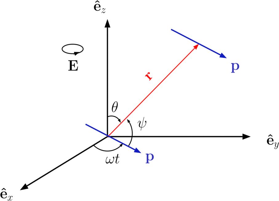
In order to introduce our model system, it is rather instructive to start with a much simplified picture of a system of ideal dipoles subject to a CP field of magnitude E0 and driven frequency ω lying along the xy plane, E = E0(êxcosωt + êysinωt), as schematically depicted in Fig. 1. We assume a stationary regime in which the point dipoles, of magnitude p0, oscillate in phase with the driven frequency, p = p0(êxcosωt + êysinωt). It is well known from basic electrostatics that, if one dipole lies at the origin of the coordinate system, the field it produces at an observation point r is E = [3(p·êr) êr − p]/r3, where êr is the unit vector pointing along the r direction.90 If another such dipole is positioned at point r, the instantaneous interacting energy between them is| | 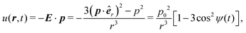 | (1) |
where ψ(t) is the instantaneous angle between the dipole moments and the dipole–dipole separation r, as depicted in Fig. 1. The radial unit vector can be expressed as êr = êxsinθcosϕ + êysinθsinϕ + êzcosθ, whereas the unit vector along the instantaneous dipole direction reads as êp = êxcosωt + êysinωt, see (Fig. 1). It follows that cosψ(t) = êr·êp = sinθ(cosφcosωt + sinφsinωt) = sinθcos(φ − ωt). Substitution of this result into eqn (1) yields| | 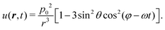 | (2) |
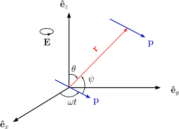 |
| | Fig. 1 Sketch of the geometry of point dipoles oscillating at angular frequency ω along a circle of radius p lying at the xy plane, and separated by a distance r. | |
Of particular physical relevance is the static, time-averaged dipole interaction ūCP(r) for circularly polarized light, which can be easily obtained by averaging the term cos2(φ − ωt) over a single rotation cycle T = 2π/ω, from which one obtains
| | 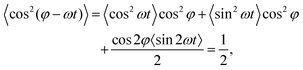 | (3) |
where we have used 〈cos
2(
ωt)〉 = 〈sin
2(
ωt)〉 = 1/2 and 〈sin(2
ωt)〉 = 0. It then follows from
(2) that the sought-for static dipole potential is
| | 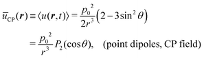 | (4) |
where
P2(cos
θ) = (3
cos
2θ − 1)/2 is the Legendre polynomial of second degree. This potential is purely repulsive when the two dipoles lie along the
z-axis and become attractive all over the
x–
y plane. In particular, we obtain
ūCP(
r,
θ = 0) =
p02/
r3 and
ūCP(
r,
θ = π/2) = −
p02/(2
r3), respectively.
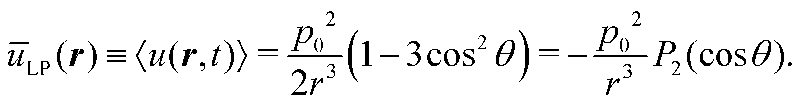
It is now instructive to compare this potential with the one of LP dipoles oscillating along the z-axis and having an oscillation amplitude p0, namely p = êzp0cosωt whereas in the CP case the dipole size remains fixed at p0 but the angle ψ(t) between the two parallel dipoles and the connecting vector varies in time, in the LP case the dipole size is time-varying while the angle θ between the two parallel dipoles and their connecting vector is time-independent. In this case, the induced interaction is u(r, t) = −E·p = p02cos2ωt(1 − 3cos2θ)/r3. After averaging the instantaneous interaction in the LP case over a period, we arrive at the static field
| |  | (5) |
The interaction is now attractive along the z-direction, and repulsive over the x–y plane: we obtain, for example, ūLP(r, θ = 0) = −p02/r3 and ūLP(r, θ = π/2) = p02/(2r3). Eqn (4) and (5) show that coefficients of P2(cosθ) in the multi-polar expansion of point dipoles differ by a sign, in spite of the quite distinctive nature of field oscillations. It should be borne in mind, however, that the angle θ has different meanings in the two cases: whereas in the LP-case θ is the angle between the vector connecting two dipoles and the fixed direction of these dipoles, in the CP-case θ stands for the angle between the connecting vector and the normal to the plane on which the dipoles are rotating. Accordingly, the change in the nature of the interactions from 1D to 2D attraction/repulsion leads, as we will establish in what follows, to quite distinct aggregation scenarios.
Despite the simple connection between CP and LP interactions expressed by eqn (4) and (5), there is a slight difference that must be taken into account when comparing these situations. While the quantity p0 in (4) stands for the magnitude of the oscillating dipole (which is fixed in time), the quantity p0 in (5) is the maximum amplitude of the oscillating dipole, which is only achieved instantaneously. Accordingly, in previous approaches that bear direct influence on the work at hand,63 the LP-interaction, both in the case of point dipoles and in that of extended ones, has been expressed in terms of the period-average p2 = p02〈cos2ωt〉 = p02/2. In terms of this quantity, the dipole interaction of point-like dipoles in the LP case reads as
| | 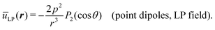 | (6) |
Comparison between eqn (4) and (6) shows that the second order coefficient of the multi-pole expansion for the CP dipole is related to its LP counterpart (of the same magnitude p0) via u(2)CP = −u(2)LP/2 when the former is expressed in terms of p0 and the latter in terms of the rsm-value p2 = p02/2. By simple symmetry arguments, it becomes clear that this correspondence must hold equally well in cases where these coefficients are functions of the radial distance between the dipoles.
Apart from its clear relation with our model system, this simplified picture of point dipoles oscillating in phase with a circularly polarized field is rather interesting on its own and shares many similarities with different systems of relevance in various applications. Consider, as an example, the interaction between ideal magnetic dipoles subject to a static magnetic field pointing along the z-axis. The induced dipole–dipole interaction between two such ideal dipoles separated by the vector r is given by u(r) = [3(êr·m)2 − m2]/r3 = m2P2(cosθ)/r3, where m is the magnitude of the magnetic dipole moment. Another interesting example is that of ideal magnetic dipoles lying on the x–y plane, under the influence of a magnetic field which oscillates over a cone surface of aperture θ with frequency ω, B = B0[(êxcosωt + êysinωt)sinθ + êzcosθ]. It is easy to verify that the interaction between the dipoles along the plane are of the form (2), with p replaced by the induce magnetic moment, and φ representing the angle with the x-axis. The static interactions thus behave like (4). Notice that, in this case, θ represents the angle between the field and the z-axis, and the particles lie along the plane. Nonetheless, it is interesting to verify that eqn (4) describes quite different situations, and the parameters therein can be adjusted to provide different arrangements of dipoles over the plane.
We now return to our model system. The simplified picture described above provides a basis to understand the more involved effective interactions between microgels induced by the CP field. As shown in ref. 63, the time-averaged, induced dipole potential between microgels under the influence of a LP field has the form
| | | ū(LP)dd(r) = u(0)dd(r) + u(2)dd(r)P2(cosθ), | (7) |
where
θ is the angle between dipoles and the connecting vector
r. As shown above, the change in geometry in the case of CP field amounts to the replacement cos
θ → cos
ψ(
t) = sin
θcos(
φ −
ωt). Following the same steps outlined above, we conclude that time averaging these quantities amounts to a simple sign change of the coefficient of
P2(cos
θ) and an overall multiplication with the factor 1/2 to express now the quantities in terms of the fixed dipole magnitude
p0. As a result, the pair interactions for the case of the CP field are readily transformed into
| | 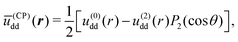 | (8) |
where
ū(CP)dd(
r) stands for the static, induced dipole interactions in the case of CP fields, the coefficients
u(0)dd(
r) and
u(2)dd(
r) are the same developed for the case of LP light but here they must be expressed in terms of the time-independent induced dipole magnitude
p0 instead of the rms-value

employed in the case of LP-fields.
The coefficients u(0)dd(r) and u(2)dd(r) are effective radial potentials, which implicitly take into account the field influence by means of two effective parameters: the strength of the induced dipole moment, p0, and the screening length κd. While the former depends on the field strength and frequency via an effective permittivity ε(ω), the latter depends only on the field frequency, which dictates the response of the free charges to the oscillating fields. This frequency-dependent inverse screening length κd can be changed from fully screened dipoles (where κd equals the static inverse Debye length) at small frequencies‡ to unscreened dipoles (in the high-frequency regime where ions do not respond to the oscillating field).
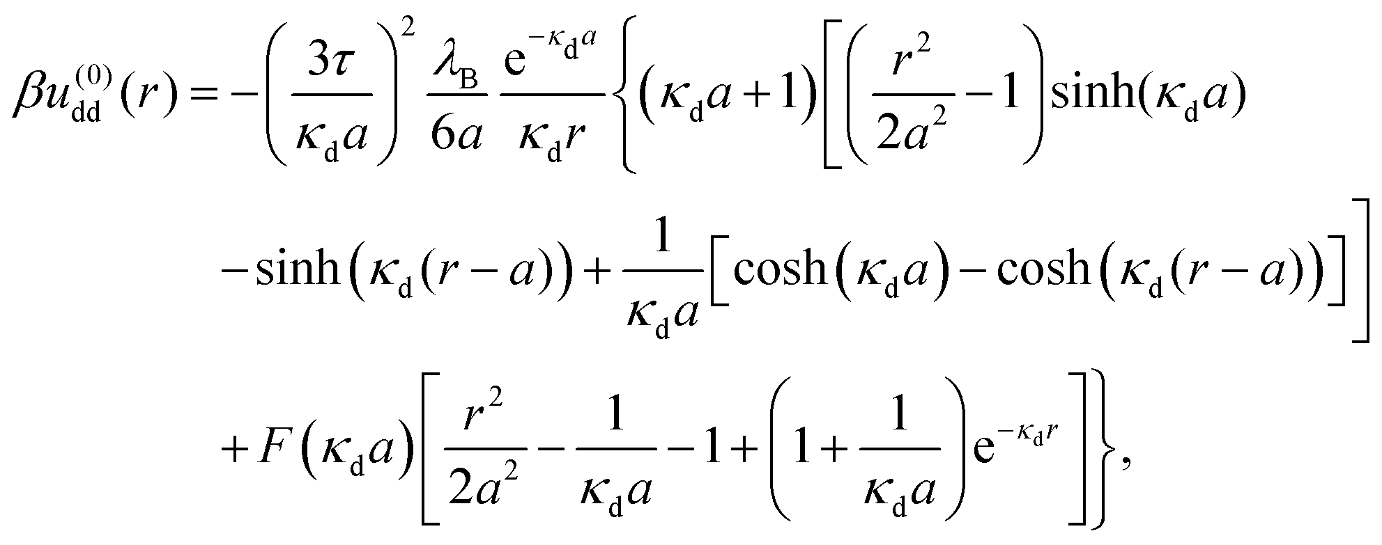
We now consider a solution of induced, extended dipoles representing ionic microgels under the influence of a AC field, immersed in a solvent of dielectric constant ε, the whole solution being at absolute temperature T and denoting β ≡ (kBT)−1 with Boltzmann's constant kB. The coefficients u(0)dd(r) and u(2)dd(r) beyond the overlapping distance (r > σ) are given by the following expressions:
| | 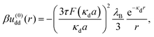 | (9) |
and
| | 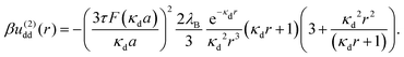 | (10) |
Here,
a =
σ/2 is the particle radius, and the function
F(
x) is defined as
F(
x) ≡
x![[thin space (1/6-em)]](https://www.rsc.org/images/entities/i_char_2009.gif)
cosh(
x) − sinh(
x) and
λB =
q2/(
εkBT) is the Bjerrum length, having the value
λB ≅ 0.71 nm for water at room temperature. The parameter
τ is defined as
τ =
p0/(
qa), and it measures the strength of the dipole moments induced by the electric field.
At overlapping distances r < σ, these coefficients read as follows:§
| |  | (11) |
and
| | 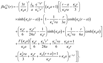 | (12) |
Since the microgels bear a uniform charge Zq, the dipole interactions above are complemented with a purely repulsive monopole interaction, in addition to an elastic repulsion upon particle overlapping. In the region r > σ, the monopole interactions read as follows:
| | 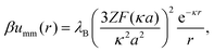 | (13) |
where
κ is the usual inverse Debye screening length. If the system is in contact with an ionic reservoir of mean concentration
cs, this quantity is given by

. As particles overlap (
r <
σ), their monopole interaction becomes
| | 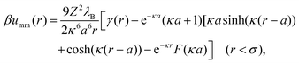 | (14) |
where the function
γ(
r) is defined as follows:
| | 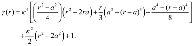 | (15) |
Finally, the soft repulsion due to the elastic interaction between overlapping polymer chains is modeled
via the de Hertz potential,
| | 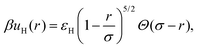 | (16) |
where
Θ(
x) is the unit step function, and
εH is a parameter which controls the strength of the soft repulsion. Throughout this work, we set this dimensionless parameter to be
εH = 800. This value is in practice high enough to prevent a significant degree of particle overlapping, which could otherwise undermine the assumptions of unscreened interactions and small deviations from sphericity. Moreover, the inverse screening length is fixed at
κ = 2.8
a−1, and the particle radius is
a = 0.53 μm. This set of parameters is shown to accurately fit the experimental data for the pair correlations between ionic microgels in the absence of external fields.
The total pair interaction between microgels induced by the external field is thus the sum of monopole, dipole and soft contributions, i.e.:
| | | βu(r) = βumm(r) + βū(CP)dd(r) + βuH(r). | (17) |
Fig. 2 displays some representative pair potentials for the case of fully screened (
κd =
κ, top panels) and unscreened (
κd = 0, bottom panels) interactions, in cases where the monopole charge is fixed at
Z = 400. The interactions are shown parallel (
Fig. 2a and c) and perpendicular (
Fig. 2b and d) to the polarization plane.
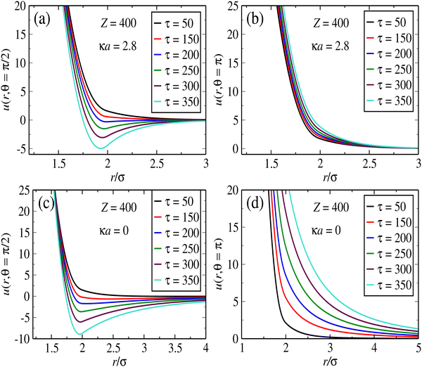 |
| | Fig. 2 Panels (a)–(d) display the potential as a function of separation distance for selected values of the angle and screening constants, as indicated in the legends. Effective potential between ionic microgels induced by a CP field, at different dipole strengths. Top panels correspond to fully screened dipole interactions (κd = κ), whereas at the bottom curves results for unscreened interactions (κ = 0) are shown. In all cases, the monopole charge is made of Z = 400 elementary charges. | |
While the interactions along the z-axis are always repulsive, the pair potential across the polarization plane features well defined potential wells at small particle separations. This short-range attraction is obviously a result of dipole interactions, which attempt to “stick together” opposite poles of neighboring particles along the equator plane. As the distance increases along this plane, the monopole repulsion becomes dominant. We notice that the potential wells have larger widths and depths in the case of unscreened interactions. That means that particles tend have more room to move along the plane in the case of unscreened dipoles. As for the screened interactions, the potential along the plane increasingly resembles that of sticky spheres as the dipole strength τ increases, since the well width becomes thinner. Likewise, the repulsion perpendicular to the polarization plane is much larger range – and becomes much more sensitive to changes in τ – in the case of unscreened interactions. It is very clear that this competition between in-plane short-range attraction and transverse repulsion should lead to sheet-like agglomerates lying parallel to the polarization plane. As we shall see, the plane formation and its inner structure can be adjusted by changing the effective parameters linked to the field properties.
4 Molecular dynamics simulation
In order to investigate the structure of microgels induced by the CP field, we employ MD simulations for a one-component system interacting through the pair interactions described in the previous section. We perform NVT simulations employing the minimum image, periodic boundary conditions, considering a cubic box containing N = 1000 particles. The simulations are performed in the fully screening limit, such that no special techniques are needed to handle the electrostatic interactions. A total of N = 50000 time-steps are employed, and averages are taken after Nm = 1000 steps, where samplings are taken in regular intervals of Ns = 1000 time-steps. Thermalization is made via by coupling the dynamics to a Andersen thermostat, in which collisions with a thermal bath are taken for randomly selected particles.91
5 The Ornstein–Zernike formalism
Additional information on the structural properties under different conditions can be very efficiently obtained by means of the Ornstein–Zernike (OZ) formalism.66 Here we outline some of the main features of this approach for the case of anisotropic interactions.
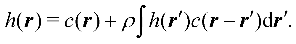
In a uniform, one component system, with effective interactions, the OZ equation relates the total h(r) and direct c(r) pair correlations as follows:
| | 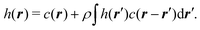 | (18) |
In Fourier space, this relation is simplified to
| |  | (19) |
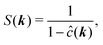
where the Fourier transforms of the pair correlations have been defined as
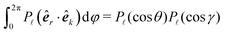
and
. The latter quantity defines the so-called structure factor, which carries information about the pattern scattering of light at a wave-vector
k and is thus amenable to scattering measurements. Due to the azimuthal symmetry, the pair correlations can be expanded as
| |  | (20) |
where
θ is the angle between
r and the
z-axis and
P![[small script l]](https://www.rsc.org/images/entities/char_e146.gif)
(cos
θ) denotes the Legendre polynomial of degree
. Invoking the addition theorem for spherical harmonics in the form
(where
γ is the angle between
k and the
z-axis), it follows that pair correlations in reciprocal space can be similarly evaluated in the form
| | 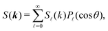 | (21) |
where the coefficients
S(
k) are related to their real space counterparts through a Henkel transform of order
,
| | 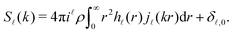 | (22) |
Similar expressions also hold for the real and reciprocal coefficients of the direct correlation
c(
r). Here,
j(
kr) represents the
-th spherical Bessel function, whose integral representation in terms of Legendre polynomials is
| | 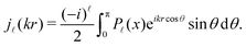 | (23) |
The set of equations above provides a useful relation between direct and total pair correlations. However, a further relation is required if one wants to calculate both quantities simultaneously. Among different closure relations, we have chosen to employ the hypernetted-chain (HNC) relation between
h(
r) and
c(
r), which in real space reads as
| | | h(r) = exp[h(r) − c(r) − βu(r)]−1. | (24) |
Before considering the expansions
(20) for the pair correlations it is convenient, for numerical proposes, to take the derivative of both sides of the above expression with respect to the radial coordinate
r:
| | 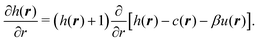 | (25) |
Expanding now both sides according to
eqn (20), and invoking the orthogonality of the functions
P(
x), we obtain
| | 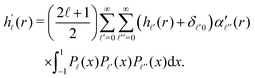 | (26) |
where
α(
r) ≡
h(
r) −
c(
r) −
βu(
r)
Now, the integral over the polar angle can be conveniently expressed in terms of the Clebsch–Gordon coefficients  . After some algebraic manipulations, we arrive at the following expression for the real space coefficients:
| | 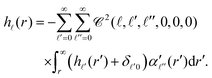 | (27) |
Together with eqn (19) and (22), the above equation provides a complete set of relations that can be used to numerically evaluate the pair correlations g(r) = 1 + h(r), c(r) and the structure factor S(k) for a given, anisotropic pair interaction u(r).
6 Results
We are now in a position to analyze in close detail the structural transitions induced by the CP field. All numerical results have been obtained at constant (room) temperature, which justifies the use of a fixed particle size throughout. Ionic thermal motion influences the relative strength of electrostatic interactions (which, in the present CG description, amounts to a shift in microgel charge), as well as the dielectric ionic response to the applied field. While these influences could in principle be accounted for by simple changes at the CG parameters, thermo-responsible microgels are known to undergo non-trivial conformation transitions upon temperature variations. Accounting for the underlying average size and packing fraction changes would require the incorporation of intriguing temperature-dependent solvent–polymer interactions, which goes beyond the scope of this work.
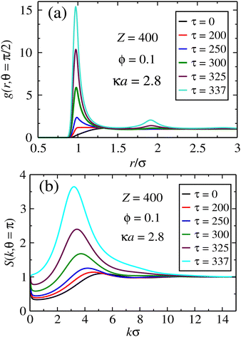
We start by looking at the in-plane and perpendicular pair correlations and structure factors, respectively, which encode information about structural transitions and particle aggregation. In Fig. 3, these quantities are shown for the case of unscreened dipoles, for a case of monopole charge Z = 400 and packing fraction of ϕ = 0.1. It is clear from Fig. 3a that particles start to come increasingly closer together at the overlapping distance r ≈ σ as their dipole moments become larger. As this parameter gets large enough, in-plane aggregation takes place. The same trend has been reported in the case of LP light, where aggregation is one-dimensional, signaling chain formation.63 In the present case, the in-plane layering implies in the formation of compact aggregates, since the correlations display radial symmetry along the plane. It is expected that, at much larger dipole strengths, in-plane crystal ordering should eventually emerge. Fig. 3b shows the corresponding structure factor in the direction normal to the polarization plane. A single peak is observed, which becomes larger and is shifted to smaller k values as the dipole strength increases. This is a signature of perpendicular (z-direction) ordering for the sheets lying on the x–y plane. The shift towards smaller k values means that the planar layers start to be farther away from one another, which also indicates that they increase in size.
 |
| | Fig. 3 Pair correlations for the case of fully screened dipoles. In (a), in-plane pair correlations indicate the formation of aggregates as τ increases, whereas in (b) the structure factors in the transversal direction suggests a 1D crystal ordering, where the in-plane aggregates stay larger apart as τ becomes larger. | |
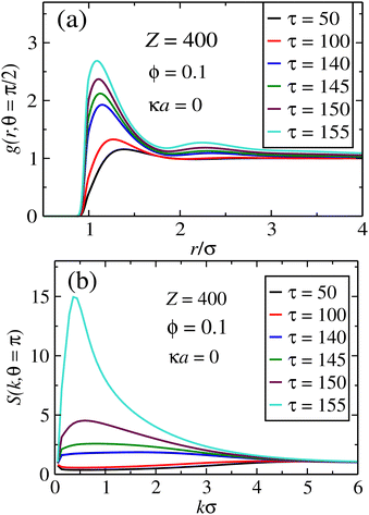
The opposite case of unscreened interactions is shown in Fig. 4, for the same set of system parameters. We now see that the heights of the pair correlations in real space are much smaller in comparison with the screened case. On the other hand, the peak of the structure factor along the perpendicular direction becomes much larger. The maximums are now much broader, indicating out-of-plane crystal formation in which the sheets are farther away from each other, with the averaged distance distributed over a wider range. It is likely that such spreading of inter-plane distances, driven by long-range interactions, results in the formation of smaller clusters along the x−y plane. This is in agreement with the smaller peaks of the in-plane pair correlations, which indicates that in average the particles will be farther apart in comparison to the fully screened situation.
 |
| | Fig. 4 Pair correlations for the case of fully unscreened dipoles. In (a), in-plane pair correlations indicate the formation of aggregates as τ increases, whereas in (b) the structure factors in the transversal direction suggests a 1D crystal ordering, where the in-plane aggregates stay larger apart as τ becomes larger. | |
There is a clear correlation between the height of the structure factor and the emergence of crystal ordering in monodisperse systems. Over the years, many different criteria (most of them of phenomenological nature) have been established in order to quantify the onset of crystal ordering.92,93 Classical examples are the Lindermann melting criterion94 and the Hansen–Verlet prescription.95 The latter establishes that, for a monodisperse particles with Lennard-Jones interactions, crystallization takes places when the height of the first peak of the structure factor reaches the threshold value S(k) ≈ 2.8. In ref. 96, this criterion has been adapted to the case of charged colloids, and it was found that the onset of crystal ordering occurs when the height if S(k) achieves values close to S(k) ≈ 2.1. Since these systems bear more similarities to our model system, we shall hereafter adopt this criterion to estimate the regions in the plane (ϕ, τ) where the parallel layers start to display ordering across the z direction. To this end, we map the regions where S(k, π = θ) ≳ 2.1 and plot the transition lines that signals the onset of 1D ordering along the perpendicular direction. The results are shown in Fig. 5, for two representative situations where Z = 100 (upper panels) and Z = 400 (lower panels), considering screened (left panels) and unscreened (right panels) interactions. Quite distinct behaviors are observed in the case of smaller screened and unscreened dipoles. As expected, screening the interactions shifts the transition lines towards larger τ values, as the interactions are weakened. When the dipole interactions are unscreened (right panels), an interesting re-entrant behavior is observed in which the liquid crystallizes and then melts up again upon increase of particle concentration. At small packing fractions and fixed τ, only a small number of sheets are able to form, and no ordering is observed. As ϕ increases, a larger number of parallel sheets are able to form, and a longitudinal ordering between them starts to emerge. At sufficiently large particle concentrations, geometric constraints should prevent addition of new particles into the layers, and some particles start to become loose between the sheets, leading to a liquid–solid coexistence.
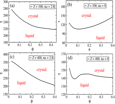 |
| | Fig. 5 Panels (a)–(d) display these lines for selected values of the angle and screening constants, as indicated in the legends. Transition lines delimiting the onset of sheet layering across the transversal direction, considering both screened and unscreened dipoles, and two representative charges of Z = 100q (top graphs) and Z = 400q (lower graphs). | |
As the charge Z increases, the monopole repulsion between the layers starts to dominate. In the case of screened interactions, the transition lines decay monotonically as ϕ increases, and the layering effect is robust against particle addition. This is no longer the case when the interactions become unscreened, as seen in Fig. 5d, which shows a rather complex layering behavior. In this case, there is a small region in which the transition line increases before moving down again. This intriguing behavior is clearly a consequence of long-range interactions. Although the repulsion is stronger among the layers, they are not localized as in the case of screened interactions, which tends to avoid layer ordering. Moreover, as shown in Fig. 4a, in-plane particle attraction is much weaker for unscreened dipoles, and particles are thereby able to get loose from the aggregates more easily.
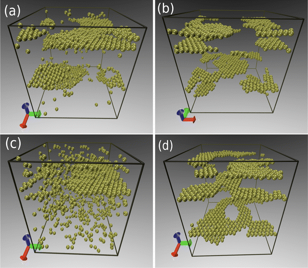
Although the transition lines based on the structure factor provide a general picture of the complex layering formation, a detailed analysis shows that, over a large region of the (ϕ, τ) plane, the layers are neither solid nor liquid, but rather a mixture of layers coexisting with a liquid of loose particles. This behavior is made clear in Fig. 6, which shows selected snapshots corresponding to points in Fig. 4a and b close to the transition lines (left panels) and deep inside the crystal region (right panels). Near the transition line, large aggregates can be observed. The sheets coexist with a gas (Fig. 6a) or a liquid (Fig. 6c) of free particles. In contrast, if one moves inside the crystal phase (Fig. 6b and d), the sheets are fully formed and no free particles are found. Moreover, the layers can display an internal crystal structure within the plane. In order to explore this rich behavior in detail, we have performed extended MD simulations over a large range of system parameters, thus mapping the different phases both transversal and parallel to the polarization plane. The results are summarized in Fig. 7 and 8, in which the different phases are shown in the (ϕ, τ) plane for the transversal layering and in-plane structures, respectively. Here, the monopole charge is fixed at Z = 90, while the interactions are fully screened. We notice in particular that a rich behavior is observed inside the aggregates, which cannot be captured within the OZ formalism. It is important to remark that predictions of OZ approach and MD simulations are in qualitative agreement regarding the layering formation (see Fig. 5c), and the dipole strengths that delimits the different phases are not too far from each other.
 |
| | Fig. 6 Snapshots representing typical simulation configurations of particles, in the case of fully screened dipoles. In all cases, the packing fraction is fixed at ϕ = 0.1. The remaining parameters are Z = 100, τ = 200 (a), Z = 100, τ = 250 (b), Z = 400, τ = 260 (c) and Z = 400, τ = 300 (d). | |
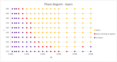 |
| | Fig. 7 Phase diagram in the (ϕ, τ) plane, detailing the layering formation along the transversal direction, obtained via MD simulations. The interactions are fully screened, and the monopole charge is set at Z = 90. | |
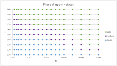 |
| | Fig. 8 Phase diagram in the (ϕ, τ) plane, showing the induced in-plane ordering behavior, as obtained from MD simulations. The interactions are fully screened, and the monopole charge is set at Z = 90. | |
The onset of sheet-like formation across the perpendicular field direction can be clearly visualized in Fig. 9, where simulation snapshots across the transition from liquid to layering formation in Fig. 7 are shown. In all cases, the packing fraction and bare charge are fixed at ϕ = 0.1 and Z = 90, while three different polarizations are considered: τ = 130 (Fig. 9a), τ = 150 (Fig. 9b) and τ = 260 (Fig. 9c). These representative points correspond to situations of no layers, emergence of layering, and fully layered structures, respectively, in Fig. 7. When the induced polarization τ is not too high, the in-plane attraction is not strong enough to overcome the monopole repulsion of equally charged particles, leading to liquid-like, amorphous structures (see Fig. 9a). As the transition line is approached (Fig. 9b), dipole interactions start to become relevant, resulting in a mixture of liquid-like and crystal orderings, characterized by the formation of small, planar agglomerates. Further increase of τ beyond this polarization threshold leads to a situation where all particles are organized into planar sheets, lying parallel to the polarization plane. Most layers feature crystal-like, in-plane ordering. Depending on field strength and packing fractions, a number of defects and holes can be observed in the planar layers, resulting from a fine competition between in-plane attraction and perpendicular repulsion between particles belonging to different layers.
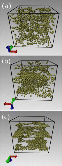 |
| | Fig. 9 Typical snapshots showing the onset of layering formation, in a situation of fixed charge (Z = 90) and packing fraction (ϕ = 0.1). The induced polarizations are τ = 130 (a), τ = 150 (b) and τ = 260 (c), representing points lying shortly before, inside, and way beyond, respectively, the transition line represented in Fig. 7. | |
7 Conclusions
We have analyzed the effective interactions and structural transitions of a system of ionic microgels subject to a CP field. To accomplish this, we have adopted a coarse-graining description similar to that applied in ref. 63 for the case of LP light. The effective interactions are comprised of (purely repulsive) monopole contributions, in addition to dipole–dipole interactions. The latter feature a short-range attraction along the polarization plane and are purely repulsive in the perpendicular direction. The dipole pair potential contains effective parameters which are closely related to the applied field, such as the dipole strength and the screening parameter of dipole interactions. Following a previous work, we expect that these parameters can be easily obtained from experimental measurements, thus allowing for a direct probe of our theoretical predictions for the structural transitions against experimental results.
Using numerical calculations based on the OZ approach and MD simulations, we were able to apply the proposed model system to investigate the various aggregation scenarios at different regions of the parameter space. A rich behavior was observed, with a re-entrant melting of plane sheets along the transversal direction, as well as in-plane transitions resulting from the short-range dipole attraction. We hope that the results herein will motivate experimental investigations for the proposed experimental setup and serve as a basis for further theoretical studies on similar systems. For example, an extension of the proposed model system can be easily worked out to incorporate different types of plane polarization, such as elliptical polarization, thus breaking up translation invariance along the polarization plane. Polydispersity is also a promising strategy to induce different structures both among layers and within the polarization plane, as the both the in-plane binding energies and the repulsion between planar sheets can be controlled by the induced dipole strength assigned to different components.
Data availability
For long-term storage of data, we will use Phaidra, the repository for the permanent secure storage of digital assets at the University of Vienna. We will therefore adhere to the standards and practices that are recommended and used there. Specifically, Phaidra uses Dublin Core and an extended LOM scheme as a metadata standard. The minimal set of metadata that are going to be employed is defined by the currently required metadata fields, as documented at https://datamanagement.univie.ac.at/en/rdm/metadata/. All metadata in Phaidra are machine readable and accessible over a standard link for each object. Documentation on accessing and using this type of information is available at the link https://github.com/phaidra/phaidra-api/wiki/Documentation.
Conflicts of interest
The authors declare no competing financial interest.
Notes and references
- T. Vicsek and F. Family, Phys. Rev. Lett., 1984, 52, 1669–1672 CrossRef.
- A. E. González, M. Lach-Hab and E. Blaisten-Barojas, J. Sol-Gel Sci. Technol., 1999, 15, 119–127 CrossRef.
- M. Grzelczak, J. Vermant, E. M. Furst and L. M. Liz-Marzán, ACS Nano, 2010, 4, 3591–3605 CrossRef CAS PubMed.
- M. F. Hagan, O. M. Elrad and R. L. Jack, J. Chem. Phys., 2011, 135, 104115 CrossRef PubMed.
- W. Jeżewski, Phys. Chem. Chem. Phys., 2015, 17, 8828–8835 RSC.
- W. Jeżewski, Phys. Chem. Chem. Phys., 2016, 18, 22929–22936 RSC.
- F. Ginot, I. Theurkauff, F. Detcheverry, C. Ybert and C. Cottin-Bizonne, Nat. Commun., 2018, 9, 696 CrossRef CAS PubMed.
- Y. Huang, C. Wu, J. Chen and J. Tang, Angew. Chem., Int. Ed., 2024, 63, e202313885 CrossRef CAS PubMed.
-
G. M. Whitesides, J. K. Kriebel and B. T. Mayers, in Self-Assembly and Nanostructured Materials, ed. W. T. S. Huck, Springer, US, Boston, MA, 2005, pp. 217–239 Search PubMed.
- O. D. Velev and S. Gupta, Adv. Mater., 2009, 21, 1897–1905 CrossRef CAS.
-
S. S. Bayram and A. S. Blum, in 12. Directing the Self-Assembly of Nanoparticles for Advanced Materials, ed. T. van de Ven and A. Soldera, De Gruyter, Berlin, Boston, 2020, pp. 307–326 Search PubMed.
- A. Rao, S. Roy, V. Jain and P. P. Pillai, ACS Appl. Mater. Interfaces, 2023, 15, 25248–25274 CrossRef CAS PubMed.
- K. Wei, Y. Shi, X. Tan, M. Shalash, J. Ren, A. A. Faheim, C. Jia, R. Huang, Y. Sheng, Z. Guo and S. Ge, Adv. Colloid Interface Sci., 2024, 332, 103271 CrossRef CAS PubMed.
- H. Cheng, R. Liu, R. Zhang, L. Huang and Q. Yuan, Nanoscale Adv., 2023, 5, 2394–2412 RSC.
- M. Singh, N. Kaur and E. Comini, J. Mater. Chem. C, 2020, 8, 3938–3955 RSC.
- A. S. Ivanov, K. G. Nikolaev, A. S. Novikov, S. O. Yurchenko, K. S. Novoselov, D. V. Andreeva and E. V. Skorb, J. Phys. Chem. Lett., 2021, 12, 2017–2022 CrossRef CAS PubMed.
- K. Jakab, C. Norotte, F. Marga, K. Murphy, G. Vunjak-Novakovic and G. Forgacs, Biofabrication, 2010, 2, 022001 CrossRef PubMed.
- A. C. Mendes, E. T. Baran, R. L. Reis and H. S. Azevedo, WIREs Nanomed. Nanobiotechnol., 2013, 5, 582–612 CrossRef CAS PubMed.
- D. T. O. Carvalho, T. Feijão, M. I. Neves, R. M. P. da Silva and C. C. Barrias, Biofabrication, 2021, 13, 035008 CrossRef CAS PubMed.
- J. Yang, H.-W. An and H. Wang, ACS Appl. Bio Mater., 2021, 4, 24–46 CrossRef CAS PubMed.
- L. Qiao, H. Yang, S. Gao, L. Li, X. Fu and Q. Wei, J. Mater. Chem. B, 2022, 10, 1908–1922 RSC.
- Y. Zhang and Q. An, Supramol. Mater., 2023, 2, 100036 Search PubMed.
- M. Rubenstein, A. Cornejo and R. Nagpal, Science, 2014, 345, 795–799 CrossRef CAS PubMed.
- B. Yigit, Y. Alapan and M. Sitti, Adv. Sci., 2019, 6, 1801837 CrossRef PubMed.
- S. Won, H. E. Lee, Y. S. Cho, K. Yang, J. E. Park, S. J. Yang and J. J. Wie, Nat. Commun., 2022, 13, 6750 CrossRef CAS PubMed.
- F. D. Guerra, M. F. Attia, D. C. Whitehead and F. Alexis, Molecules, 2018, 23, 1760 CrossRef PubMed.
- A. Thamizhanban, G. P. Sarvepalli, K. Lalitha, Y. S. Prasad, D. K. Subbiah, A. Das, J. B. Balaguru Rayappan and S. Nagarajan, ACS Omega, 2020, 5, 3839–3848 CrossRef CAS PubMed.
- Y. Cho, Y. Son, J. Ahn, H. Lim, S. Ahn, J. Lee, P. K. Bae and I.-D. Kim, ACS Nano, 2022, 16, 19451–19463 CrossRef CAS PubMed.
- N. J. W. Penfold, J. Yeow, C. Boyer and S. P. Armes, ACS Macro Lett., 2019, 8, 1029–1054 CrossRef CAS PubMed.
- S. Varlas, T. J. Neal and S. P. Armes, Chem. Sci., 2022, 13, 7295–7303 RSC.
- V. L. Morales, J.-Y. Parlange, M. Wu, F. J. Pérez-Reche, W. Zhang, W. Sang and T. S. Steenhuis, Langmuir, 2013, 29, 1831–1840 CrossRef CAS PubMed.
- M. Farrokhbin, B. Stojimirović, M. Galli, M. Khajeh Aminian, Y. Hallez and G. Trefalt, Phys. Chem. Chem. Phys., 2019, 21, 18866–18876 RSC.
- T. Curk and E. Luijten, Phys. Rev. Lett., 2021, 126, 138003 CrossRef CAS PubMed.
- K. Barros and E. Luijten, Phys. Rev. Lett., 2014, 113, 017801 CrossRef CAS PubMed.
- H.-K. Kwon, B. Ma and M. Olvera de la Cruz, Macromolecules, 2019, 52, 535–546 CrossRef CAS.
- B. Ma and M. Olvera de la Cruz, J. Phys. Chem. B, 2021, 125, 3015–3022 CrossRef CAS PubMed.
- E. Lopez-Fontal, A. Grochmal, T. Foran, L. Milanesi and S. Tomas, Chem. Sci., 2018, 9, 1760–1768 RSC.
- J. Feng, Y. Qiu, H. Gao and Y. Wu, Acc. Chem. Res., 2024, 57, 222–233 CrossRef CAS PubMed.
- A. M. R. Kabir, K. Sada and A. Kakugo, Chem. Commun., 2021, 57, 468–471 RSC.
- H. S. Yun, D. H. Kim, H. G. Kwon and H. K. Choi, Macromolecules, 2022, 55, 4305–4312 CrossRef CAS.
- E. Axell, J. Hu, M. Lindberg, A. J. Dear, L. Ortigosa-Pascual, E. A. Andrzejewska, G. Šneideriene, D. Thacker, T. P. J. Knowles, E. Sparr and S. Linse, Proc. Natl. Acad. Sci. U. S. A., 2024, 121, e2322572121 CrossRef CAS PubMed.
- G. Cravotto and P. Cintas, Chem. Soc. Rev., 2009, 38, 2684–2697 RSC.
- Y. Chen, X. Ding, S.-C. Steven Lin, S. Yang, P.-H. Huang, N. Nama, Y. Zhao, A. A. Nawaz, F. Guo, W. Wang, Y. Gu, T. E. Mallouk and T. J. Huang, ACS Nano, 2013, 7, 3306–3314 CrossRef CAS PubMed.
- T. J. Woehl, K. L. Heatley, C. S. Dutcher, N. H. Talken and W. D. Ristenpart, Langmuir, 2014, 30, 4887–4894 CrossRef CAS PubMed.
- Z. Arnon, S. Piperno, D. Redeker, E. Randall, A. Tkachenko, H. Shpaisman and O. Gang, Nat. Commun., 2024, 15, 6875 CrossRef CAS PubMed.
- P. M. Adriani and A. P. Gast, Faraday Discuss. Chem. Soc., 1990, 90, 17–29 RSC.
- D. Heinrich, A. R. Goñi, T. M. Osán, L. M. C. Cerioni, A. Smessaert, S. H. L. Klapp, J. Faraudo, D. J. Pusiol and C. Thomsen, Soft Matter, 2015, 11, 7606–7616 RSC.
- D. Xu, R. Shi, Z.-Y. Sun and Z.-Y. Lu, J. Chem. Phys., 2021, 154, 144904 CrossRef CAS PubMed.
- B. Li, Y.-L. Wang, G. Shi, Y. Gao, X. Shi, C. E. Woodward and J. Forsman, ACS Nano, 2021, 15, 2363–2373 CrossRef CAS PubMed.
- A. A. Harraq, B. D. Choudhury and B. Bharti, Langmuir, 2022, 38, 3001–3016 CrossRef CAS PubMed.
- C. Dalle-Ferrier, M. Krüger, R. D. L. Hanes, S. Walta, M. C. Jenkins and S. U. Egelhaaf, Soft Matter, 2011, 7, 2064–2075 RSC.
- F. Evers, R. D. L. Hanes, C. Zunke, R. F. Capellmann, J. Bewerunge, C. Dalle-Ferrier, M. C. Jenkins, I. Ladadwa, A. Heuer, R. Castañeda-Priego and S. U. Egelhaaf, Eur. Phys. J.: Spec. Top., 2013, 222, 2995–3009 Search PubMed.
- P. S. Mohanty, P. Bagheri, S. Nöjd, A. Yethiraj and P. Schurtenberger, Phys. Rev. X, 2015, 5, 011030 Search PubMed.
- P. Gadige and R. Bandyopadhyay, Soft Matter, 2018, 14, 6974–6982 RSC.
- M. Marć, A. Drzewiński, W. W. Wolak, L. Najder-Kozdrowska and M. R. Dudek, Nanomaterials, 2021, 11, 1737 CrossRef PubMed.
-
K. M. Krishnan, Fundamentals and Applications of Magnetic Materials, Oxford University Press, 2016 Search PubMed.
- X. Liu, N. Kent, A. Ceballos, R. Streubel, Y. Jiang, Y. Chai, P. Y. Kim, J. Forth, F. Hellman, S. Shi, D. Wang, B. A. Helms, P. D. Ashby, P. Fischer and T. P. Russell, Science, 2019, 365, 264–267 CrossRef CAS PubMed.
- Ž. Gregorin, N. Sebastián, N. Osterman, P. Hribar Boštjančič, D. Lisjak and A. Mertelj, J. Mol. Liq., 2022, 366, 120308 CrossRef.
-
W. B. Russel, D. A. Saville and W. R. Schowalter, Colloidal Dispersions, Cambridge University Press, 1989 Search PubMed.
- S. Vesaratchanon, A. Nikolov and D. T. Wasan, Adv. Colloid Interface Sci., 2007, 134–135, 268–278 CrossRef CAS PubMed.
- J. K. Whitmer and E. Luijten, J. Chem. Phys., 2011, 134, 034510 CrossRef PubMed.
- C. M. Alexander, J. C. Dabrowiak and J. Goodisman, J. Colloid Interface Sci., 2013, 396, 53–62 CrossRef CAS PubMed.
- T. Colla, P. S. Mohanty, S. Nöjd, E. Bialik, A. Riede, P. Schurtenberger and C. N. Likos, ACS Nano, 2018, 12, 4321–4337 CrossRef CAS PubMed.
- K. Jathavedan, S. K. Bhat and P. S. Mohanty, J. Colloid Interface Sci., 2019, 544, 88–95 CrossRef CAS PubMed.
- J. R. Maestas, F. Ma, N. Wu and D. T. Wu, ACS Nano, 2021, 15, 2399–2412 CrossRef CAS PubMed.
-
J. P. Hansen and I. McDonald, Theory of Simple Liquids, Academic, London, 1990 Search PubMed.
- L. A. Rosen and D. A. Saville, Langmuir, 1991, 7, 36–42 CrossRef CAS.
- C. Cametti, Soft Matter, 2011, 7, 5494–5506 RSC.
- P. S. Mohanty, S. Nöjd, M. J. Bergman, G. Nägele, S. Arrese-Igor, A. Alegria, R. Roa, P. Schurtenberger and J. K. G. Dhont, Soft Matter, 2016, 12, 9705–9727 RSC.
- S. N. Ashrafizadeh, Z. Seifollahi, A. Ganjizade and A. Sadeghi, Electrophoresis, 2020, 41, 81–103 CrossRef CAS PubMed.
- T. D. Nguyen and M. Olvera de la Cruz, ACS Nano, 2019, 13, 9298–9305 CrossRef CAS PubMed.
- I. M. Telles and A. P. dos Santos, Langmuir, 2021, 37, 2104–2110 CrossRef CAS PubMed.
- P. S. Mohanty, A. Yethiraj and P. Schurtenberger, Soft Matter, 2012, 8, 10819–10822 RSC.
- S. Nöjd, P. S. Mohanty, P. Bagheri, A. Yethiraj and P. Schurtenberger, Soft Matter, 2013, 9, 9199–9207 RSC.
- J. J. Crassous, A. M. Mihut, E. Wernersson, P. Pfleiderer, J. Vermant, P. Linse and P. Schurtenberger, Nat. Commun., 2014, 5, 5516 CrossRef CAS PubMed.
- C. N. Likos, Soft Matter, 2006, 2, 478–498 RSC.
- J. Bohlin, A. J. Turberfield, A. A. Louis and P. Šulc, ACS Nano, 2023, 17, 5387–5398 CrossRef CAS PubMed.
- D. Gottwald, C. N. Likos, G. Kahl and H. Löwen, J. Chem. Phys., 2005, 122, 074903 CrossRef CAS PubMed.
- J. Riest, P. Mohanty, P. Schurtenberger and C. N. Likos, Z. Phys. Chem., 2012, 226, 711–735 CrossRef CAS.
- G. Agrawal and R. Agrawal, Polymers, 2018, 10, 418 CrossRef PubMed.
- D. Gottwald, C. N. Likos, G. Kahl and H. Löwen, Phys. Rev. Lett., 2004, 92, 068301 CrossRef CAS PubMed.
- T. Colla, R. Blaak and C. N. Likos, Soft Matter, 2018, 14, 5106–5120 RSC.
- E. Maza, C. von Bilderling, M. L. Cortez, G. Daz, M. Bianchi, L. I. Pietrasanta, J. M. Giussi and O. Azzaroni, Langmuir, 2018, 34, 3711–3719 CrossRef CAS PubMed.
- C. Misra, S. V. Kawale, S. K. Behera and R. Bandyopadhyay, Phys. Fluids, 2024, 36, 103120 CrossRef CAS.
- M. Urich and A. R. Denton, Soft Matter, 2016, 12, 9086–9094 RSC.
- Y. Levin, A. Diehl, A. Fernández-Nieves and A. Fernández-Barbero, Phys. Rev. E: Stat., Nonlinear, Soft Matter Phys., 2002, 65, 036143 CrossRef PubMed.
- T. Colla, C. N. Likos and Y. Levin, J. Chem. Phys., 2014, 141, 234902 CrossRef PubMed.
- A. R. Denton and Q. Tang, J. Chem. Phys., 2016, 145, 164901 CrossRef PubMed.
- M. O. Alziyadi and A. R. Denton, J. Chem. Phys., 2023, 159, 184901 CrossRef CAS PubMed.
-
J. D. Jackson, Classical Electrodynamics, Wiley, New York, NY, 3rd edn, 1999 Search PubMed.
-
D. Frenkel and B. Smit, Understanding Molecular Simulation: From Algorithms to Applications, Academic Press, Inc., USA, 1st edn, 1996 Search PubMed.
- H. Löwen, Phys. Rep., 1994, 237, 249–324 CrossRef.
- A. K. Arora and B. Tata, Adv. Colloid Interface Sci., 1998, 78, 49–97 CrossRef CAS.
- S. Rabinovich, D. Berrebi and A. Voronel, J. Phys.: Condens. Matter, 1989, 1, 6881 CrossRef.
- J.-P. Hansen and L. Verlet, Phys. Rev., 1969, 184, 151–161 CrossRef CAS.
- R. Kesavamoorthy, B. Tata, A. Arora and A. Sood, Phys. Lett. A, 1989, 138, 208–212 CrossRef CAS.
Footnotes |
| † This paper is dedicated to the memory of Stefan U. Egelhaaf, dear colleague and esteemed physicist, whose contributions to the understanding of the structure and dynamics of colloidal suspensions have been an inspiration for us. |
| ‡ Here, small or large frequencies are to be compared with the typical inverse diffusion times of ions in solution. |
| § There is a typo in the expression for u(0)dd(r) in ref. 63. The last term in the outer brackets therein contains an erroneous extra factor of κda in front of F(κda). The expression shown here is the correct one and all calculations have been performed with the correct expression in ref. 63. |
|
| This journal is © The Royal Society of Chemistry 2025 |
Click here to see how this site uses Cookies. View our privacy policy here. 
 Open Access Article
 This Open Access Article is licensed under a Creative Commons Attribution-Non Commercial 3.0 Unported Licence
 *b and
Christos N.
Likos
*b and
Christos N.
Likos
 where ρ denotes the average concentration of these particles. Upon close contact, the spheres interact (in addition to electrostatic interactions) via a soft potential due to the elastic repulsion between their polymer networks. Neither volume changes nor particle deformations from the spherical shape are considered. The surrounding electrolyte is considered under the framework of the linearized Debye–Hückel approach, which is known to work rather well in the present case of weakly charged, stiff microgels with uniform charges.79 It is important to note that the underlying assumptions of sphericity and unscreened interactions become inaccurate in cases of ultra-soft microgels, i.e., those synthesized with a small concentration of cross-linkers. In these cases, the CG approach has to be modified to take account of anisotropic conformation changes driven by both external fields and particle interactions. Moreover, the high degree of penetrability leads to unscreened electrostatic interactions upon overleaping. In order to avoid these shortcomings, we shall henceforth confine our attention to stiff microgels, in which case deviations from both sphericity and unscreened interactions can be neglected. We consider isotropic media, in which case the dielectric properties are described through a scalar, frequency-dependent permittivity. The applied CP field will induce polarizing charges, described through the formation of oscillating charges of opposite signs at the particle surface. Ignoring higher-order terms on the charge multi-polar expansion, we consider the formation of a (static) surface charge of the form σ(θ) = σ0


 employed in the case of LP-fields.


 . As particles overlap (r < σ), their monopole interaction becomes


 and
and  . The latter quantity defines the so-called structure factor, which carries information about the pattern scattering of light at a wave-vector k and is thus amenable to scattering measurements. Due to the azimuthal symmetry, the pair correlations can be expanded as
 (where γ is the angle between k and the z-axis), it follows that pair correlations in reciprocal space can be similarly evaluated in the form


 . After some algebraic manipulations, we arrive at the following expression for the real space coefficients:


