DOI:
10.1039/D5SM00201J
(Paper)
Soft Matter, 2025,
21, 5947-5956
Defect dynamics in dry active nematics by residue calculus for holomorphic functions of nematic director field
Received
25th February 2025
, Accepted 24th June 2025
First published on 26th June 2025
Abstract
This paper proposes a theory for modeling the dynamics of topological defects in dry active nematics. We introduce a holomorphic function for integral curves of the director field and show the density of the integral curves corresponds to that of active nematic liquid crystals such as confined spindle-shaped cells. Then, we derive equations of motion for defects by considering active stress defined from the integral curves. A mathematical analysis of the equations reveals that the dynamics of the defects can be explicitly expressed with the residues of holomorphic functions derived from the director field. We verify the proposed theory using existing work on the motion of a defect pair and demonstrate estimation of parameters for active stress by cell culture experiments.
1 Introduction
Recent studies in the field of biophysics and non-equilibrium physics have revealed that living or actively moving nematic liquid crystals induce complex fluidic and mechanical phenomena known as active nematics.1–3 The complex behavior of active nematics is governed by topological defects, at which the alignment of nematic liquid crystals cannot be defined. Active stress induced by components of an active nematic system creates a force acting on topological defects, resulting in self-propelled motion of the defects. Many studies have investigated the dynamics of defect motion for various active nematic systems such as compounds of kinesins and microtubules,4–8 spindle-shaped cell populations9–20 and morphogenesis of Hydra.21,22
To theoretically explain the complex behavior of active nematics, many studies applied complex analysis,23–38 because the alignment of nematic liquid crystals can be expressed by complex logarithmic functions under the one-constant approximation in liquid crystal theories.39 Complex analysis has enabled the explicit expression of the alignment of nematic liquid crystals24,27,30–33 and the force and torque acting on topological defects.23,25,26,28,29,35–38 According to the explicit expressions based on complex analysis, equations for defect motion have been derived, which allow a detailed theoretical analysis of defect behaviors.
Theoretical studies of defect motion have considered passive and active stresses caused by the elasticity and mechanical deformation of nematic liquid crystals, respectively, and the equations of motion were then derived from the force acting on defects by the passive stress and Stokes flow caused by the active stress to model “wet” active nematics where the conservation of momentum is considered.23,37 In these studies, the density of the active nematic liquid crystals was assumed to be constant for simplicity in the theoretical calculations. On the other hand, the densities of the components tend to be non-uniform around topological defects in actual active nematic systems. Such non-uniformity is often observed in cell populations at a confluent state; for example, neural progenitor cells show aggregation and escape behaviors around +1/2 and −1/2 defects, around which the cell alignment angle changes by +180° and −180°, respectively.11 In addition, some studies reported observations of extrusion of spatially confined cells around a +1/2 defect in MDCK cells10 and a +1 defect in mouse myoblast cells.12 These studies support the non-uniformity of components of cell populations which can be viewed as “dry” active nematic systems,1 where substrate friction is dominant and thus the conservation of momentum does not hold. To theoretically study the dynamics of topological defects in cell populations, new theoretical approaches are necessary to consider the non-uniform distribution of components in dry active nematics.
The aim of this study is to develop a theoretical framework for defect motion in dry active nematic systems that considers the orientational continuity and density of liquid crystals in a simple manner. To this end, we extend the work of Vitelli and Nelson, who introduced a complex potential to express such continuous lines from a holomorphic function for nematic alignment.40 We show that such a formalism provides an explicit expression of active stress based on holomorphic functions and that the densities of the constructed continuous lines increase and decrease around +1/2 and −1/2 defects, respectively, which is qualitatively consistent with the experimental observations of cell populations in the literature.11 In addition, we demonstrate that the proposed formalism enables both mathematical analyses of defect motion and the prediction of the active stress parameter from cell culture experiments.
This paper is organized as follows. In Section 2, we introduce a holomorphic function for modeling density of liquid crystals around topological defects by extending the work of Vitelli and Nelson.40 In Section 3, we show that the active stress can be explicitly expressed by the introduced holomorphic function defined in Section 2. In Section 4, we demonstrate the validity of the proposed theory using existing work on the motion of a defect pair studied by Giomi et al.23 In Section 5, we consider the confinement of liquid crystals in simply connected domains and show that the proposed theory can be extended to the confined geometries considered in existing studies.9,16,20 In Section 6, we show that the extended theory for confined nematic liquid crystals can be applied to the prediction of the active stress parameter from cell culture experiments.
The mathematical notation in this paper is as follows.  and
and  represent the sets of integers, and real and complex numbers, respectively. For a complex number
  the real and imaginary parts of z are expressed as Re[z] and Im[z], respectively.
  denotes the open unit disk in the complex ζ-plane.
2 Complex function theory for nematic director field around topological defects
First, we consider the alignment of nematic liquid crystals in the complex plane z = x + iy, whose director field is defined as nd(x, y) = (cos![[thin space (1/6-em)]](https://www.rsc.org/images/entities/char_2009.gif) ϕ(x, y), sinϕ(x, y))T. We assume that the size of the nematic liquid crystals is neglected. Since the nematic liquid crystals are non-polar molecules, we assume that the alignment angle ϕ is defined in the quotient space
ϕ(x, y), sinϕ(x, y))T. We assume that the size of the nematic liquid crystals is neglected. Since the nematic liquid crystals are non-polar molecules, we assume that the alignment angle ϕ is defined in the quotient space  that is, ϕ is equivalent to ϕ + mπ for any
  . In this paper, we consider the one-constant approximation from liquid crystal theory,39 which allows us to assume that the alignment angle ϕ(x, y) is harmonic. Then, the alignment angle ϕ(x, y) can be expressed by taking the real part of a holomorphic function f(z) = ϕ(x, y) + iψ(x, y), where ψ(x, y) is a conjugate harmonic function of ϕ(x, y). Based on the report of Vitelli and Nelson,40 we can construct continuous lines whose tangential orientation at (x, y) is parallel to the orientation of the director field nd(x, y) according to the following procedures. Let us consider a following holomorphic function defined from f(z):
| | | h′(z) = Aexp(−if(z)) = Aeψ(cosϕ − isinϕ) | (1) |
where  and A is an arbitrary real non-zero constant. Since the coefficient Aeψ is real, the vector field nh(x, y) = (Aeψcosϕ, Aeψsinϕ)T defined from (1) represents the director field scaled by the factor Aeψ. Thus, we refer to the vector field nh(x, y) as the holomorphic director field in this paper. Accordingly, h(z) is called the complex potential for the holomorphic director field.
By considering the contours of the imaginary part of h(z), we can obtain the integral curves of the holomorphic director field nh(x, y),40 whose tangential orientation is parallel to the orientation of the director field nd(x, y). That is, the integral curves are given by the following contour line:
| |  | (2) |
This fact is proven mathematically by the following procedure. For a line element ds on (2), we have
| |  | (3) |
It holds from
(1) and (3) that
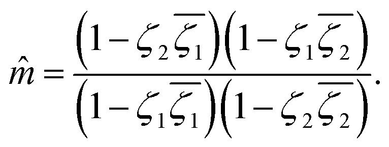
| |  | (4) |
Using |d
z/d
s| = 1 and
(4), we have d
z/d
s = e
iϕ or d
z/d
s = −e
iϕ = e
i(ϕ+π). Since
ϕ and
ϕ + π are equivalent in the quotient space

the tangential derivative d
z/d
s is parallel to the director field
nd(
x,
y) on the contour line Im[
h(
z)] =
c. This means the tangential direction at
z =
x +
iy on the contour line Im[
h(
z)] =
c is parallel to the director field
nd(
x,
y). We refer to the contours of Im[
h(
z)] as integral curves of the holomorphic director field
nh(
x,
y) (hereinafter, referred to simply as integral curves).
In the following, we investigate the mathematical and physical meaning of the constructed integral curves for some simple examples. When the nematic liquid crystals are aligned along the real axis, ϕ(x, y) is equal to zero for all z, which means f(z) = 0 and h′(z) = Aexp(−if(z)) = A. Then, the complex potential h(z) is equal to Az + c, where c is an arbitrary constant and we set c = 0 throughout this paper without loss of generality. Since the imaginary part of h(z) is Ay, the contour lines are parallel to the real axis and uniformly distributed as shown in Fig. 1(a). Note that the density of the contour lines in Fig. 1(a) differs according to the absolute value of A because the slope of the contour lines is A. Thus, the parameter |A| represents the density of the integral curves when there are no topological defects in the space.
 |
| | Fig. 1 Schematics of director field and integral curves. (a) No defect. (b) +1/2 defect. (c) −1/2 defect. The black lines in the director field and integral curves indicate the orientation of the director and contours of Im[h(z)], respectively. The contour interval is 0.05. | |
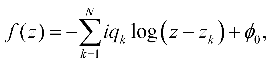
Next, we consider the alignment around a topological defect around which the alignment angle changes by 2πq, where q is a half or full non-zero integer, called the topological charge. In this case, the alignment angle around the defect is expressed as the real part of f(z) = −iqlogz. Then, the complex potentials h(z) around a defect with topological charges of q = +1/2 and −1/2 are given as follows:
| |  | (5) |
We refer to these two defects as +1/2 and −1/2 defects in this paper. The contours of Im[
h(
z)] are shown in
Fig. 1(b) and (c). In contrast to
Fig. 1(a), the contours around the +1/2 and −1/2 defects become denser and sparser toward the origin, respectively.
The difference in the density occurs because the density of the contours of Im[h(z)] ≡Ψ(x, y) is proportional to the magnitude of its gradient |∇Ψ(x, y)| = |h′(z)|. For ±1/2 defects, the gradient in polar coordinates z = reiθ is calculated as
| |  | (6) |
Thus, when we consider the limit of
r → 0, |
h′(
z)| diverges to +∞ for
q = +1/2 whereas |
h′(
z)| converges to 0 for
q = −1/2, which is consistent with
Fig. 1(b) and (c).
Note that the non-uniform density of the integral curves around +1/2 defects is qualitatively consistent with experiments on active nematics in extrusion of MDCK cells10 and aggregation of neural progenitor cells around +1/2 defects.11 Thus, the proposed formulation is a plausible approach for the theoretical investigation of dry active nematics from the viewpoint of the density of the integral curves.
3 Representations of passive and active stresses by residue calculus
In the following section, we investigate the representation of passive and active stresses in studying the dynamics of defect motion driven by forces acting on topological defects. For this, we assume that N topological defects exist in the complex z-plane. Then, the director of the nematic alignment is expressed by| |  | (7) |
where  is some real constant, and zk and qk are the location and topological charge of the k-th defect, respectively. We also denote a small disk with a radius of ε that includes only a k-th defect as Dk(ε), which is referred to as a defect core. According to Giomi et al.,23 we have to consider two forces due to elastic and active stress. For the elastic stress, Denniston41 derived the passive force (Fpx, Fpy)T in a complex form for the topological defect located at z = zk as follows:
| |  | (8) |
where K is the Frank elastic constant and ![[f with combining circumflex]](https://www.rsc.org/images/entities/i_char_0066_0302.gif) k(z) ≡ f(z) + iqklog(z − zk) is a function f(z) except for the logarithmic singularity at z = zk. This formula is also applicable to simply and doubly connected domains with infinite anchoring conditions on the boundaries.42
k(z) ≡ f(z) + iqklog(z − zk) is a function f(z) except for the logarithmic singularity at z = zk. This formula is also applicable to simply and doubly connected domains with infinite anchoring conditions on the boundaries.42
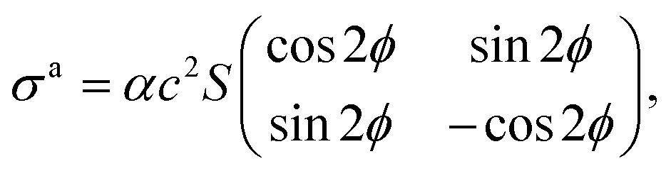
On the other hand, the active stress generated by self-propelled particles is expressed as
| |  | (9) |
where
S is the scalar order parameter,
c is the concentration of the particles and
α is a constant that is positive or negative for contractile or extensile motion, respectively.
23,43 Note that the existing studies
23,43 assumed that the density of the self-propelled particles was constant, which implies that the spatial change in the force was not explicitly considered. To appropriately model the non-uniformity of the force around topological defects, the density of the integral lines of the holomorphic director field
nh should be considered. This consideration is reasonable because the driving force for active nematics is generated by extensile or contractile behaviors of elongated cells, which can be viewed as the integral lines of
nh. To this end, we consider the force generated by self-propelled particles on the integral lines and assume that the density of self-propelled particles on a line is proportional to the density of the integral lines. Since the density of the integral lines is proportional to |
h′(
z)| = e
ψ, as discussed above, we assume that the concentration
c in
(9) is proportional to e
ψ. The active stress tensor for the holomorphic director field
nh is then given by
| |  | (10) |
In
(10), the scalar order parameter
S is merged into
α because
S is assumed to be constant outside the defect core
Dk(
ε) in theoretical analyses.
28 In addition, the parameter
α is rescaled to
α/2 to simplify the following calculation.
Using the derived stress tensor ![[small sigma, Greek, circumflex]](https://www.rsc.org/images/entities/i_char_e111.gif) a, the active force applied to defects can be explicitly expressed in the same way as the elastic force derived by Denniston.41 The force applied to Dk(ε) is given by
a, the active force applied to defects can be explicitly expressed in the same way as the elastic force derived by Denniston.41 The force applied to Dk(ε) is given by
| |  | (11) |
where
![[n with combining circumflex]](https://www.rsc.org/images/entities/b_i_char_006e_0302.gif)
is a normal vector on the boundary ∂
Dk(
ε). Using
= (cos
θ, sin
θ)
T on the point
z =
zk +
εe
iθ ∈ ∂
Dk(
ε) and applying a direct calculation, the force due to active stress is
| |  | (12) |
where we used d
z =
iεe
iθd
θ. It follows from
(8) and (12) that the force acting on the defect is given by the following formula
| |  | (13) |
This formula means that the forces acting on defects are determined by residues of the two holomorphic functions
f′(
z)
2 and
h′(
z)
2, which are derived from the two director fields
nd(
x,
y) and
nh(
x,
y), respectively.
4 Theoretical analyses on motion of a defect pair
Based on the derived formula for the forces, the equations of defect motion can be explicitly expressed as follows. In this treatment, we consider the defect dynamics of the dry active nematics, where the substrate friction is dominant and thus the conservation of the momentum does not hold. According to the existing study of Duclos et al.,9 the substrate friction is dominant in confined cell populations, which means the defect dynamics in confined cell populations can be modeled as dry active nematics. The defect dynamics of dry active nematics, where the effects of hydrodynamics are neglected, can be expressed using the following overdamped equation of motion:| |  | (14) |
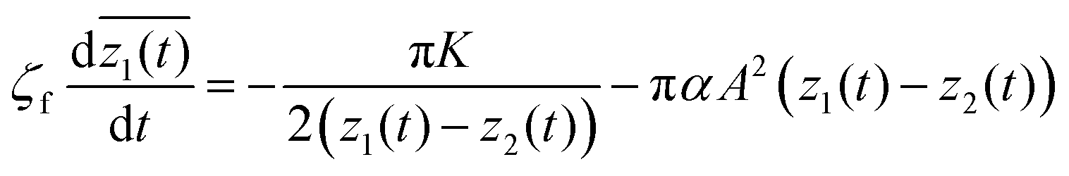
where ζf is a frictional constant.23 To verify consistency with the work of Giomi et al.,23 we consider the case of two topological defects with opposite signs on an infinite plane. The holomorphic function for the director field nd(x, y) is given by| |  | (15) |
where z1(t) and z2(t) are the positions of the defects with charges of ±1/2 at time t, and the alignment angle becomes π/2 in the far-field. By definition, we have| |  | (16) |
The integral curves around the defect pair are obtained by analytically integrating (16) with respect to z, which gives| |  | (17) |
Calculating the residues of f′(z)2 and h′(z)2 at each defect, the equations of motion are derived as follows:
| |  | (18) |
| |  | (19) |
The solutions of
(18) and (19) simulate the temporal movement of the two defects, as shown in
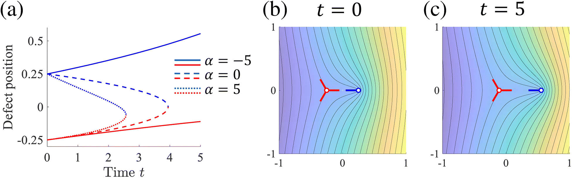
Fig. 2(a).
Fig. 2(b) and (c) show a typical behavior of extensile motion (
α < 0). Because of the active stress term with negative
α, the topological defect with +1/2 moves away from the other defect, which follows the distortion of the integral curves around the +1/2 defect.
 |
| | Fig. 2 Motion of a defect pair. (a) Time evolution of z1(t) and z2(t) for K = 1, A = 1 and ζf = 100. The blue and red lines represent z1(t) and z2(t), respectively. (b) and (c) Integral curves around the defect pair for α = −5 calculated from (17). | |
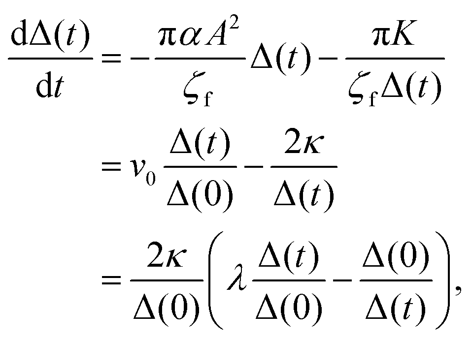
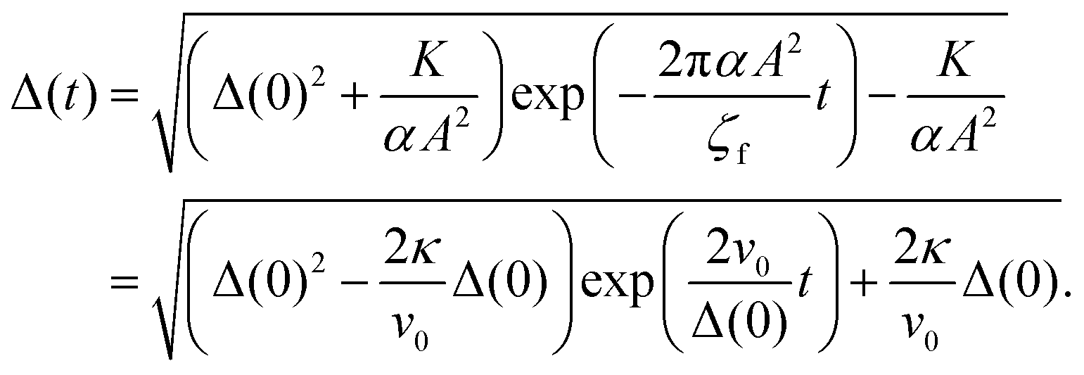
It is difficult to analytically solve the simultaneous differential eqn (18) and (19). However, the dynamics of the pair separation Δ(t) := x1(t) − x2(t) can be solved in closed form under the assumption that the two defects are located on the real axis. By subtracting (19) from (18), the differential equation of the separation Δ(t) is given by
| | 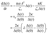 | (20) |
where
v0 := −π
αA2Δ(0)/
ζf,
κ := π
K/(2
ζf) and
λ :=
v0Δ(0)/2
κ. Since the derived
eqn (20) is in the form of a Bernoulli differential equation when
α ≠ 0,
(20) is analytically solved as follows:
| |  | (21) |
The solid lines in
Fig. 3(a) show the typical time course of the solution
(21) when the contractile active stress (
i.e. v0 ∝ −
α < 0) is considered. The annihilation time shortens as the constant
κ increases. Moreover, the annihilation of the defect pair can be predicted by setting the right-hand side of the solution
(21) equal to zero. When
α > −
K/(
A2Δ(0)
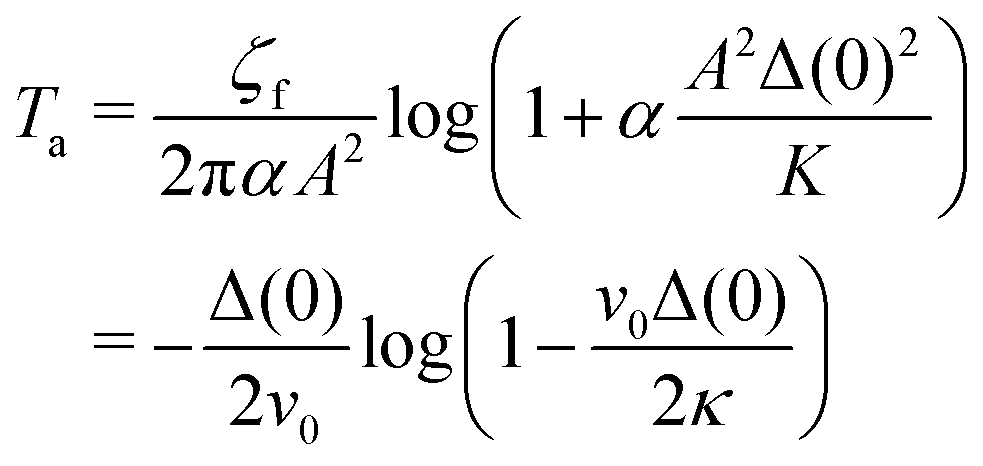
2), the defect pair is annihilated at the following time
Ta:
| |  | (22) |
In the limit of
α → 0, the annihilation time becomes
T0a =
ζfΔ(0)
2/(2π
K) = Δ(0)
2/4
κ, which is consistent with the annihilation of a defect pair in passive nematic systems.
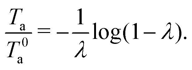
23 The annihilation time normalized by
T0a depends only on the non-dimensional quantity
λ =
v0Δ(0)/2
κ as follows:
| |  | (23) |
Fig. 3 shows the relationship between the parameter −
λ and the normalized annihilation time
(23).
 |
| | Fig. 3 Dynamics of the defect separation when contractile active stress is considered. (a) Time course of the defect separation Δ(t) for v0 = −0.1 and various constants κ. The solid and dotted lines represent the solutions of the eqn (20) and (24), respectively. To solve (24), ode23s in MATLAB® was used. (b) Relationship between the parameter −λ and the normalized annihilation time Ta/T0a. | |
We next compare the derived differential eqn (20) with the existing work of Giomi et al.23 According to Giomi et al., the equation of the pair separation Δ(t) is given as follows:
| |  | (24) |
where
v0 ∝ −
α is the constant self-propelled velocity of the +1/2 defect,
κ := π
K/(2
ζf) and
λ :=
v0Δ(0)/2
κ. The dotted lines in
Fig. 3 show the solutions of
(24) and indicate that the annihilation time for
(24) shortens compared to that for
(20) when the same parameters
v0,
κ and Δ(0) are used. The normalized annihilation time for
(24) is calculated as follows:
| |  | (25) |
The normalized annihilation time for
(24) is always less than that for
(20) as shown in
Fig. 3. This difference between
(20) and (24) is due to the first term in the right-hand side, which is derived from the active stress. Specifically, the first term in
(24) is constant, whereas that in
(20) is proportional to the normalized separation Δ(
t)/Δ(0). Thus, the contribution of the active stress in the proposed model
(20) becomes small when Δ(
t) goes to zero, whereas the contribution of the active stress in
(24) remains constant even when Δ(
t) goes to zero. As the contribution of the contractile active stress enhances the annihilation of defect pairs, the normalized annihilation time for
(24) will become shorter than that for
(20). This difference in the first term may be critical when the two defects are far away from each other. However, the comparison between our and Giomis results (
Fig. 3) implies that the difference between the two models is not significant, with the same trend of defect pair annihilation reproduced in the proposed model, which indicates there is not a serious gap between the proposed theory and Giomi's model when the defects are located close to each other.
Note that the above difference between our and Giomi's approaches is due to the difference between dry and wet active nematics, respectively. Giomi et al. considered the flow dynamics induced by the active and passive stresses and then solved the dynamics of the defect pair, whereas we neglected the hydrodynamics and considered that the velocities of the defects are directly proportional to the forces acting on the defects. Thus, our approach cannot be applied to the complex behaviors of active turbulence observed in compounds of microtubules and kinesins4–8 because the conservation of momentum should be considered in such active fluid. Though the proposed model can consider only dry active nematics, it has an advantage from the viewpoint of analytic calculations. Since Giomi et al. considered the Stokes flow induced by the external active stress around a single defect, they needed to calculate the line integrals regarding the Oseen tensor. This approach would be more difficult for more complex defect configurations, such as defects in confined geometries. In contrast, our formalism focuses on direct calculation of the forces acting on defects, which results in a simple evaluation of the residues of the holomorphic functions at each defect. This simplified approach allows us to investigate the motion of defects of confined cell populations in more complicated domains, as will be discussed in the following section.
5 Equilibrium states of topological defects in confined geometries
We investigate the equilibrium states of defect motion in confined geometries, which have been investigated for elongated cell populations.9,10,12,16,20 Specifically, we consider two +1/2 defects located at ζ = ζ1,ζ2 in a unit disk  , with its image mapped by a conformal mapping of z = g(ζ). According to our previous studies,20,32 the holomorphic function for the director field nd(x, y) in
  is expressed by
| |  | (26) |
where  is the holomorphic function of the director field in
  given by
| |  | (27) |
From (1) and (27), we have
| |  | (28) |
Thus, the complex potential for the holomorphic director field in

is obtained by
| |  | (29) |
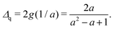
where

is an incomplete elliptic integral of the first kind and
| |  | (30) |
| |  | (31) |
Fig. 4(a) shows the integral lines of the derived potential

. The line density around the +1/2 defects increases, which is similar to
Fig. 1.
 |
| | Fig. 4 Integral curves in confined geometries. (a) Unit disk  . (b) Domain Ω mapped from the unit disk by the function g(ζ) = ζ + 0.3ζ3. (c) Domain Ω mapped from the unit disk by the function . (b) Domain Ω mapped from the unit disk by the function g(ζ) = ζ + 0.3ζ3. (c) Domain Ω mapped from the unit disk by the function  where a = 1.1. where a = 1.1. | |
Using the derived potential  the complex potential in the mapped domain
  can be calculated as follows. It follows from the definition (1) that
| |  | (32) |
Then, we have
| |  | (33) |
Eqn (33) means that the complex potential for the holomorphic director field
h(
z) is conformally invariant, whereas the holomorphic function associated with the director field
f(
z) is not conformally invariant due to the correction term −
ilog
g′(
g−1(
z)) in
fΩ(
z).
Fig. 4(b) and (c) show examples of the integral curves in
Ω.
To study the equilibrium state of the defect motion, we focus on the force acting on two +1/2 defects at z = ±g(r), (0 < r < 1). When the defect motion is at equilibrium, the total force applied to each defect should be equal to zero. By calculating the residues of  and
and  around the defect at z = +g(r), the elastic and active forces applied to the defect at z = +g(r) can be calculated from (13) as follows:
| |  | (34) |
where
![[small alpha, Greek, circumflex]](https://www.rsc.org/images/entities/i_char_e101.gif)
≡
α/
K. By setting the above force
(34) equal to zero, we obtain the following equation to satisfy the equilibrium condition:
| |  | (35) |
Thus, the equilibrium point
z = +
g(
r) is calculated by solving
(35) with respect to
r and mapping the solution by
g(
ζ). The equilibrium point depends on the parameter
. Conversely, if we obtain the equilibrium point +
g(
r) from experiments, the parameter
can be explicitly estimated from
(35) as follows:
| |  | (36) |
6 Estimation of active stress parameter from cell culture experiments
We demonstrate the validity of the proposed estimation method for the active stress parameter using two existing studies16,20 which observed the alignment of mouse myoblast cells (C2C12 cells) in closed domains. In our previous study,20 we considered the domain Ω mapped from the unit disk  by the function z = g(ζ) = ζ + βζ3 (0 ≤ β < 1/3) as shown in Fig. 5(a). Note that the area of the domain Ω was normalized to that of the unit disk
  , and the length scale in the experiments was normalized by taking 300 μm to be equal to 1, as in the previous study.20
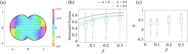 |
| | Fig. 5 Estimation of the parameter from the experiments of stable defect positions in mouse myoblast cells.20 (a) Cell alignment in the domain Ω mapped from the unit disk  by the function g(ζ) = ζ + βζ3. Note that the area of the domain Ω is normalized to that of the unit disk by the function g(ζ) = ζ + βζ3. Note that the area of the domain Ω is normalized to that of the unit disk  . Blue circles represent +1/2 defects. (b) Box plots of horizontal defect positions for various geometrical parameters β. (c) Box plots of the predicted parameter from (38). Red cross marks indicate outliers. We used Chebfun44 for calculating the inverse map ζ = g−1(z). . Blue circles represent +1/2 defects. (b) Box plots of horizontal defect positions for various geometrical parameters β. (c) Box plots of the predicted parameter from (38). Red cross marks indicate outliers. We used Chebfun44 for calculating the inverse map ζ = g−1(z). | |
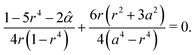
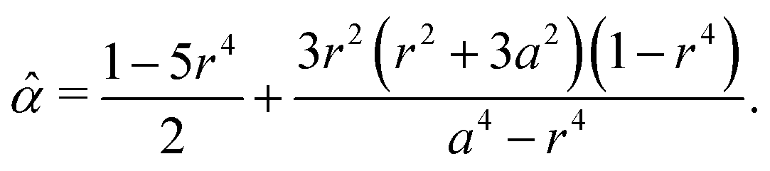
From (35), the equilibrium point z = +g(r) is calculated by solving the following algebraic equation.
| |  | (37) |
Fig. 5(b) shows the calculated equilibrium point for 0 ≤
β < 1/3 and the experimental results from our previous study, which investigated defect positions in mouse myoblast cells.
20 The experimental results are smaller than the theoretically calculated positions without active stress (
= 0). As the active stress increases (
= 0.3, 0.4), the theoretical and experimental results become matched. According to
(36), the estimation formula for
is given as follows:
| |  | (38) |
Fig. 5(c) shows box plots of the estimated parameter
, whose median is around 0.4 to 0.5. The interquartile range increases as the geometrical parameter
β increases, which indicates the uncertainty of the estimation tends to increase as the geometry becomes more asymmetric.
Other work by Ienaga et al.16 considered two overlapping circular boundaries, mathematically modeled as quadrature domains and expressed by the following conformal mapping from the unit disk  :34
:34
| |  | (39) |
where
a > 1.
Fig. 6(a) shows an example of cell alignment in the quadrature domain. According to cell culture experiments,
16 the distance
D++ between the two +1/2 defects was fitted by the distance
Δq between the centers of the two circles as follows:
| |  | (40) |
where the distance
Δq is expressed as
| |  | (41) |
On the other hand, the equilibrium point
z = +
D++/2 = +
g(
r) is theoretically calculated by solving the following equation:
| |  | (42) |
Fig. 6(b) shows the experimental and theoretical distances
D++ between the two +1/2 defects in terms of the distance
Δq. Similarly to
Fig. 5, the experimental values are lower than the theoretical values without active stress (
= 0). It follows from
(42) that the parameter
is estimated by the following equation.
| |  | (43) |
The estimated parameter
ranged between 0.1 and 0.5 and varied with the distance
Δq (
Fig. 6(c)).
 |
| | Fig. 6 Estimation of the parameter from the experiments of stable defect positions in mouse myoblast cells in the domain where two disks intersect.16 (a) Cell alignment in the domain Ω mapped from the unit disk  by the function (39). Blue circles represent +1/2 defects. (b) Distance D++ between the two +1/2 defects for various geometrical parameters Δq. For each Δq, the parameter a is obtained by solving (41). (c) Predicted parameter from (43) with a parameter r obtained by solving D++/2 = g(r). by the function (39). Blue circles represent +1/2 defects. (b) Distance D++ between the two +1/2 defects for various geometrical parameters Δq. For each Δq, the parameter a is obtained by solving (41). (c) Predicted parameter from (43) with a parameter r obtained by solving D++/2 = g(r). | |
In the above two examples, the parameter is estimated to be positive, which implies that the myoblast cells generate contractile stress. These results are consistent with an existing study on the defect dynamics in free space, which reported that the direction of defect motion in C2C12 cells was opposite to that in neural progenitor cells, which show extensile active behaviors.11 Thus, the proposed estimation method shows promise for quantifying the degree of contractility or extensibility of cell populations using only the equilibrium states of defects. In contrast to an existing study of the quantification of active nematics which considered an integer defect in a small circle,45 the proposed method can be applied to arbitrary simply connected domains. This advantage helped reveal the possibility that the active stress parameter depends on the domain geometry (Fig. 5 and 6). However, the uncertainty of the estimated was very large in Fig. 5 and 6. In particular, the estimated changed by a factor of five in Fig. 6, possibly because the experimental results of the distance D++ was fitted by a simple line in the study16 and the error of the fitting is not considered in the estimation of . In addition to the explicit formulas for the estimation of (38) and (43), some statistical approaches will also be necessary to capture the distributions of observed defects for a more precise estimation of , which will be a focus of our future work. Though further experimental research is needed to validate the estimated parameter , our theory revealed that the force acting on a defect can be expressed as residues of complex functions and enabled a detailed analysis of defect dynamics and the estimation of the activeness, which cannot be achieved by numerical simulations. Thus, the proposed theory will open up an analytical approach for investigating the essential dynamics of topological defects in active nematics.
7 Conclusions
This paper proposed a new theoretical framework to mathematically model defect motion by constructing integral curves defined from the director field of a dry active nematic system based on complex analysis. As a result, we revealed that defect motion is characterized by the residues of two holomorphic functions derived from the director field. Moreover, the proposed method reproduced and refined the theory of defect motion for a defect pair and was able to estimate the active stress from the results of cell culture experiments.
In this paper, we modeled the density of active nematic liquid crystals as the densities of integral lines of the holomorphic director field to qualitatively consider the increase and decrease of cell densities around +1/2 and −1/2 defects, respectively. However, we could not offer an evaluation or comparison of the line densities in the experiments because the size of the nematic liquid crystals is neglected in the proposed theory whereas the size of cells should be considered in actual experiments. An additional limitation is that the spatial variation of the density of the proposed integral lines cannot be controlled and thus the proposed integral lines cannot be precisely fitted to the experimental data because the spatial distributions of the integral lines are determined by the complex function f(z), which is derived from the director field nd under the one constant approximation. Thus, further analytic tools are required to bridge the gap between the proposed theoretical model and actual cell experiments to investigate how the density variations affect the defect dynamics.
For the analysis of the defect dynamics, we considered torque-free motion of a defect pair and ignored the direction of the defects in this paper. However, many studies have found that torques around defects play an important role in the complex dynamics of defect motion.25,26,28,29,38 Thus, our future work will include an extension of the proposed theory to include the effects of torques around defects. In addition, cell culture experiments are required to verify the theoretical predictions of defect motion and estimated active stress parameter .
Author contributions
H. Miyazako: conceptualization, formal analysis, resources, writing original draft; H. Miyoshi: conceptualization, formal analysis, writing original draft; T. N.: conceptualization, supervision, review & editing. All authors gave final approval for publication and agree to be held accountable for the work performed therein.
Conflicts of interest
There are no conflicts to declare.
Data availability
The program code for this study is available in Zenodo and can be accessed via this link https://doi.org/10.5281/zenodo.15779307.
Acknowledgements
The first author was supported in part by the Japan Society for the Promotion of Science KAKENHI (grant numbers JP23H00086 and JP23H04406) and JST, PRESTO Grant Number JPMJPR24KB, Japan. The second author was supported by a Postdoctoral Research Fellowship from the Japan Society for the Promotion of Science (JSPS-24KJ0041).
References
- A. Doostmohammadi, J. Ignés-Mullol, J. M. Yeomans and F. Sagués, Nat. Commun., 2018, 9, 3246 CrossRef PubMed
 .
.
- J. Zhao, U. Gulan, T. Horie, N. Ohmura, J. Han, C. Yang, J. Kong, S. Wang and B. B. Xu, Small, 2019, 15, e1900019 CrossRef PubMed .
- A. Doostmohammadi and B. Ladoux, Trends Cell Biol., 2022, 32, 140–150 CrossRef CAS PubMed .
- T. Sanchez, D. T. N. Chen, S. J. DeCamp, M. Heymann and Z. Dogic, Nature, 2012, 491, 431–434 CrossRef CAS PubMed .
- J. Hardoüin, R. Hughes, A. Doostmohammadi, J. Laurent, T. Lopez-Leon, J. M. Yeomans, J. Ignés-Mullol and F. Sagués, Commun. Phys., 2019, 2, 121 CrossRef .
- A. J. Tan, E. Roberts, S. A. Smith, U. A. Olvera, J. Arteaga, S. Fortini, K. A. Mitchell and L. S. Hirst, Nat. Phys., 2019, 15, 1033–1039 Search PubMed .
- A. Sciortino, L. J. Neumann, T. Krüger, I. Maryshev, T. F. Teshima, B. Wolfrum, E. Frey and A. R. Bausch, Nat. Mater., 2023, 22, 260–268 CrossRef CAS PubMed .
- I. Vélez-Cerón, P. Guillamat, F. Sagués and J. Ignés-Mullol, Proc. Natl. Acad. Sci. U. S. A., 2024, 121, e2312494121 CrossRef PubMed .
- G. Duclos, C. Erlenkämper, J.-F. Joanny and P. Silberzan, Nat. Phys., 2017, 13, 58–62 Search PubMed .
- T. B. Saw, A. Doostmohammadi, V. Nier, L. Kocgozlu, S. Thampi, Y. Toyama, P. Marcq, C. T. Lim, J. M. Yeomans and B. Ladoux, Nature, 2017, 544, 212–216 CrossRef CAS PubMed .
- K. Kawaguchi, R. Kageyama and M. Sano, Nature, 2017, 545, 327–331 CrossRef CAS PubMed .
- P. Guillamat, C. Blanch-Mercader, G. Pernollet, K. Kruse and A. Roux, Nat. Mater., 2022, 21, 588–597 CrossRef CAS PubMed .
- V. Yashunsky, D. J. G. Pearce, C. Blanch-Mercader, F. Ascione, P. Silberzan and L. Giomi, Phys. Rev. X, 2022, 12, 041017 CAS .
- J.-M. Armengol-Collado, L. N. Carenza, J. Eckert, D. Krommydas and L. Giomi, Nat. Phys., 2023, 19, 1773–1779 Search PubMed .
- K. Kaiyrbekov, K. Endresen, K. Sullivan, Z. Zheng, Y. Chen, F. Serra and B. A. Camley, Proc. Natl. Acad. Sci. U. S. A., 2023, 120, e2301197120 CrossRef CAS PubMed .
- R. Ienaga, K. Beppu and Y. T. Maeda, Soft Matter, 2023, 19, 5016–5028 RSC .
- T. Sarkar, V. Yashunsky, L. Brézin, C. Blanch Mercader, T. Aryaksama, M. Lacroix, T. Risler, J.-F. Joanny and P. Silberzan, PNAS Nexus, 2023, 2, gad034 CrossRef PubMed .
- M. Riedl, I. Mayer, J. Merrin, M. Sixt and B. Hof, Nat. Commun., 2023, 14, 5633 CrossRef CAS PubMed .
- C.-L. Lv, Z.-Y. Li, S.-D. Wang and B. Li, Commun. Phys., 2024, 7, 351 CrossRef .
- H. Miyazako, K. Tsuchiyama and T. Nara, npj Biol. Phys. Mech., 2024, 1, 1 CrossRef .
- Y. Maroudas-Sacks, L. Garion, L. Shani-Zerbib, A. Livshits, E. Braun and K. Keren, Nat. Phys., 2021, 17, 251–259 Search PubMed .
- Z. Wang, M. C. Marchetti and F. Brauns, Proc. Natl. Acad. Sci. U. S. A., 2023, 120, e2220167120 CrossRef CAS PubMed .
- L. Giomi, M. J. Bowick, P. Mishra, R. Sknepnek and M. Cristina Marchetti, Philos. Trans. R. Soc., A, 2014, 372, 20130365 CrossRef PubMed .
- A. J. Vromans and L. Giomi, Soft Matter, 2016, 12, 6490–6495 RSC .
- X. Tang and J. V. Selinger, Soft Matter, 2017, 13, 5481–5490 RSC .
- X. Tang and J. V. Selinger, Soft Matter, 2019, 15, 587–601 RSC .
- A. H. Lewis, D. G. A. L. Aarts, P. D. Howell and A. Majumdar, Stud. Appl. Math., 2017, 138, 438–466 CrossRef .
-
F. Vafa, M. J. Bowick, M. C. Marchetti and B. I. Shraiman, arXiv, 2020, preprint, [cond-mat.soft] DOI:10.48550/arXiv.2007.02947.
- F. Vafa, Soft Matter, 2022, 18, 8087–8097 RSC .
- O. S. Tarnavskyy, M. F. Ledney and A. I. Lesiuk, Liq. Cryst., 2018, 45, 641–648 CrossRef CAS .
- O. S. Tarnavskyy and M. F. Ledney, Liq. Cryst., 2023, 50, 21–35 CrossRef CAS .
- H. Miyazako and T. Nara, R. Soc. Open Sci., 2022, 9, 211663 CrossRef PubMed .
- H. Miyazako and T. Sakajo, Proc. R. Soc. A, 2024, 480, 20230879 CrossRef .
- H. Miyoshi, H. Miyazako and T. Nara, Proc. R. Soc. A, 2024, 480, 20240405 CrossRef .
- T. G. J. Chandler and S. E. Spagnolie, J. Fluid Mech., 2023, 967, A19 CrossRef CAS .
- T. G. J. Chandler and S. E. Spagnolie, SIAM J. Appl. Math., 2024, 84, 2476–2501 CrossRef .
- J. Rønning, C. M. Marchetti, M. J. Bowick and L. Angheluta, Proc. R. Soc. A, 2022, 478, 20210879 CrossRef PubMed .
- S. Čopar and Ž. Kos, Soft Matter, 2024, 20, 6894–6906 RSC .
-
P. G. de Gennes and J. Prost, The physics of liquid crystals, Clarendon Press, Oxford, England, 2nd edn, 1995 Search PubMed .
- V. Vitelli and D. R. Nelson, Phys. Rev. E:Stat., Nonlinear, Soft Matter Phys., 2006, 74, 021711 CrossRef CAS PubMed .
- C. Denniston, Phys. Rev. B: Condens. Matter Mater. Phys., 1996, 54, 6272–6275 CrossRef CAS PubMed .
- H. Miyoshi, D. G. Crowdy, H. Miyazako and T. Nara, Proc. R. Soc. A, 2025, 481, 20240569 CrossRef .
- R. Aditi Simha and S. Ramaswamy, Phys. Rev. Lett., 2002, 89, 058101 CrossRef CAS PubMed .
-
T. A. Driscoll, N. Hale and L. N. Trefethen, Chebfun Guide, Pafnuty Publications, 2014 Search PubMed .
- C. Blanch-Mercader, P. Guillamat, A. Roux and K. Kruse, Phys. Rev. Lett., 2021, 126, 028101 CrossRef CAS PubMed .
Footnote |
| † These authors contributed equally to this work. |
|
| This journal is © The Royal Society of Chemistry 2025 |
Click here to see how this site uses Cookies. View our privacy policy here. 
 Open Access Article
 This Open Access Article is licensed under a
  *,
Hiroyuki
Miyoshi†
and
Takaaki
Nara
*,
Hiroyuki
Miyoshi†
and
Takaaki
Nara
 and
and  represent the sets of integers, and real and complex numbers, respectively. For a complex number
  the real and imaginary parts of z are expressed as Re[z] and Im[z], respectively.
  denotes the open unit disk in the complex ζ-plane.
 that is, ϕ is equivalent to ϕ + mπ for any
  . In this paper, we consider the one-constant approximation from liquid crystal theory,39 which allows us to assume that the alignment angle ϕ(x, y) is harmonic. Then, the alignment angle ϕ(x, y) can be expressed by taking the real part of a holomorphic function f(z) = ϕ(x, y) + iψ(x, y), where ψ(x, y) is a conjugate harmonic function of ϕ(x, y). Based on the report of Vitelli and Nelson,40 we can construct continuous lines whose tangential orientation at (x, y) is parallel to the orientation of the director field nd(x, y) according to the following procedures. Let us consider a following holomorphic function defined from f(z):
 and A is an arbitrary real non-zero constant. Since the coefficient Aeψ is real, the vector field nh(x, y) = (Aeψ


 the tangential derivative dz/ds is parallel to the director field nd(x, y) on the contour line Im[h(z)] = c. This means the tangential direction at z = x + iy on the contour line Im[h(z)] = c is parallel to the director field nd(x, y). We refer to the contours of Im[h(z)] as integral curves of the holomorphic director field nh(x, y) (hereinafter, referred to simply as integral curves).


 is some real constant, and zk and qk are the location and topological charge of the k-th defect, respectively. We also denote a small disk with a radius of ε that includes only a k-th defect as Dk(ε), which is referred to as a defect core. According to Giomi et al.,23 we have to consider two forces due to elastic and active stress. For the elastic stress, Denniston41 derived the passive force (Fpx, Fpy)T in a complex form for the topological defect located at z = zk as follows:
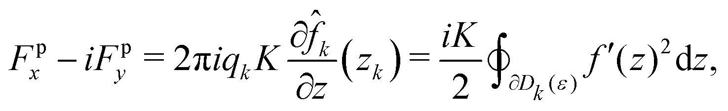


 , with its image mapped by a conformal mapping of z = g(ζ). According to our previous studies,20,32 the holomorphic function for the director field nd(x, y) in
  is expressed by
 is the holomorphic function of the director field in
  given by

 is obtained by
 is an incomplete elliptic integral of the first kind and
 . The line density around the +1/2 defects increases, which is similar to Fig. 1.

 . (b) Domain Ω mapped from the unit disk by the function g(ζ) = ζ + 0.3ζ3. (c) Domain Ω mapped from the unit disk by the function
  where a = 1.1.
 the complex potential in the mapped domain
  can be calculated as follows. It follows from the definition (1) that

 and
and 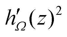 around the defect at z = +g(r), the elastic and active forces applied to the defect at z = +g(r) can be calculated from (13) as follows:


 by the function z = g(ζ) = ζ + βζ3 (0 ≤ β < 1/3) as shown in Fig. 5(a). Note that the area of the domain Ω was normalized to that of the unit disk
  , and the length scale in the experiments was normalized by taking 300 μm to be equal to 1, as in the previous study.20

 by the function g(ζ) = ζ + βζ3. Note that the area of the domain Ω is normalized to that of the unit disk
  . Blue circles represent +1/2 defects. (b) Box plots of horizontal defect positions for various geometrical parameters β. (c) Box plots of the predicted parameter

 :34
:34


 by the function (39). Blue circles represent +1/2 defects. (b) Distance D++ between the two +1/2 defects for various geometrical parameters Δq. For each Δq, the parameter a is obtained by solving (41). (c) Predicted parameter