
Elastic instability of wormlike micelle solution flow in serpentine channels†
Emily Y.
Chen
 a and
Sujit S.
Datta
*ab
a and
Sujit S.
Datta
*ab
aDepartment of Chemical and Biological Engineering, Princeton University, Princeton, NJ 08544, USA
bDivision of Chemistry and Chemical Engineering, California Institute of Technology, Pasadena, CA 91125, USA. E-mail: ssdatta@caltech.edu
First published on 22nd May 2025
Abstract
Wormlike micelle (WLM) solutions are abundant in energy, environmental, and industrial applications, which often rely on their flow through tortuous channels. How does the interplay between fluid rheology and channel geometry influence the flow behavior? Here, we address this question by experimentally visualizing and quantifying the flow of a semi-dilute WLM solution in millifluidic serpentine channels. At low flow rates, the base flow is steady and laminar, with strong asymmetry and wall slip. When the flow rate exceeds a critical threshold, the flow exhibits an elastic instability, producing spatially-heterogeneous, unsteady three-dimensional (3D) flow characterized by two notable features: (i) the formation and persistence of stagnant but strongly-fluctuating and multistable “dead zones” in channel bends, and (ii) intermittent 3D “twists” throughout the bulk flow. The geometry of these dead zones and twisting events can be rationalized by considering the minimization of local streamline curvature to reduce flow-generated elastic stresses. Altogether, our results shed new light into how the interplay between solution rheology and tortuous boundary geometry influences WLM flow behavior, with implications for predicting and controlling WLM flows in a broad range of complex environments.
1. Introduction
Above a threshold concentration in solution, many surfactants self-assemble into long, flexible, polymer-like chains reaching microns in length. However, unlike polymers, these wormlike micelles (WLMs) constantly break and reform at thermal equilibrium and under flow. Hence, they are often termed “living polymers”.1,2 When concentrated enough to be semi-dilute, WLM solutions are both strongly shear thinning and highly elastic, and therefore, are used in a wide range of energy and industrial applications, such as subsurface proppant transport,3–6 groundwater remediation,7,8 heating and cooling,9–11 drag reduction,12–16 lubrication,17 drug manufacturing and delivery,18–20 and as rheological modifiers in consumer products.4,14,21,22All of these applications involve the flow of WLM solutions through complex, confined spaces, such as winding pipes and porous rocks, where the boundary geometry introduces tortuosity to the flow. This tortuous flow in turn couples to the complex WLM solution rheology to produce unusual flow behaviors. For example, in Couette-type geometries, the homogeneous base flow can become unstable, separating into low and high shear bands that together maintain a constant shear stress with increasing shear rate23–28—a form of shear localization. The high shear rate band can subsequently exhibit another instability that produces unsteady flow,26,29–33 with pronounced spatiotemporal fluctuations similar to those exhibited by elastic polymer solutions in tortuous spaces.34–40 This instability arises at low Reynolds number (Re ≪ 1)—so the effects of inertia, which often causes flow instabilities, are negligible. Instead, it is generated by fluid elasticity, and is therefore often parameterized by the Weissenberg number, Wi, which compares the relative strength of elastic and viscous stresses. This purely-elastic instability has also been documented for WLM solutions flowing in a range of microfluidic geometries, such as through rectangular channels,41,42 around sharp bends,43,44 through contractions and expansions,45,46 in cavities,47 and past a single obstacle48–55 or two-dimensional (2D) array of obstacles.56–58 However, such geometries have multiple confounding factors, such as mixed shear and extensional flow topology and the presence of stagnation points at solid surfaces, that can simultaneously influence the flow behavior. Thus, a clear understanding of how the coupling between tortuous boundary geometry and fluid rheology influences the complex flow behavior of WLM solutions is still lacking.
Here, we simplify this problem by studying WLM solution flow at Re ≪ 1 and Wi ∼ 1 in serpentine channels comprising successive semi-circular half-loops. This microfluidic geometry enables us to isolate the role of fluid streamline curvature—which is known to be a key factor controlling purely-elastic flow instabilities since it generates elastic hoop stresses36,37—in shaping the unstable flow. Indeed, our work is inspired by prior studies of elastic instabilities in polymer solutions;59–64 these provide useful intuition, but are not directly reflective of the flow behavior of WLM solutions, which have fundamentally different microstructures and rheological properties. We find that the base steady, laminar flow exhibits strong asymmetry and wall slip at the lowest flow rates tested due to the unique rheology of the WLM solution, which enables it to support shear localization. Above a critical Wi = Wic, the flow becomes unstable, producing spatially-heterogeneous unsteady three-dimensional (3D) flow. This unsteady flow has two notable features: (i) persistent, fluctuating dead zones, which form due to the ability of the WLM solution to support shear localization, and (ii) slow “twisting” events in 3D. Our characterization of these unusual flow behaviors suggests that when WLM solutions are forced to flow in confined, tortuous spaces, they develop pathways of least resistance that minimize local streamline curvature. Altogether, our work provides a key first step toward making sense of complex fluid flows in complex spaces, potentially enabling their prediction and control in a broad range of applications.
2. Methods
2.1. Test fluid and preparation
We use a well-characterized semi-dilute, entangled WLM solution composed of 100 mM cetylpyridinium chloride (CPyCl; Sigma-Aldrich) and 60 mM sodium salicylate (NaSal; Sigma-Aldrich) in ultrapure Millipore water.45–47,51,52,58,65–70 We prepare the solution by first dissolving the CPyCl, which is a cationic surfactant, and then adding the NaSal, an aromatic organic salt, and stirring the solution for 24 h. The addition of NaSal induces the elongation of micelles due to electrostatic screening of the charged headgroups and steric interaction with the aromatic ring of the organic salt.70 We let the resulting WLM solution rest for >48 h to allow air bubbles to disappear before use. We also add 1 μm diameter fluorescent, amine-functionalized polystyrene tracer particles (Invitrogen; yellow-green) to the solution at 20 ppm for flow visualization and particle image velocimetry (PIV).2.2. Shear rheology
To characterize the shear rheology of the WLM solution, we use a stress-controlled Anton Paar MCR501 rheometer fitted with a truncated cone-plate geometry (CP50-2: 50 mm diameter, 2°, 53 μm) at a controlled temperature of 25 °C. We measure steady-state flow curves at fixed values of the shear rate![[small gamma, Greek, dot above]](https://www.rsc.org/images/entities/i_char_e0a2.gif) , ramping up and down between 0.01 and 10 s−1; shear rates exceeding 10 s−1 result in fluid ejection due to an elastic instability. The results, averaged over three replicate measurements, are shown in Fig. 1(a) and (b). As shown in Fig. 1(a), the shear stress σ increases approximately linearly with shear rate up to 0 ≈ 0.3 s−1, and then plateaus at a value σ* = 13 Pa, a signature that may reflect the presence of shear banding.24–27 As we show later on, this strong shear thinning of the WLM solution has an important consequence for its flow in serpentine channels: it enables them to support shear localization, i.e., separate into low and high shear regions under a constant imposed bulk flow rate. As shown in Fig. 1(b), the corresponding dynamic viscosity η() = σ()/ is nearly constant at η0 = 49 Pa s at low shear rates, and then continually decreases (shear thinning) with increasing > 0. This shear thinning behavior is described well by the Carreau–Yasuda model,71 as demonstrated in previous studies of similar or identical WLM solutions;49,51,54,55,58,69,72 the model is shown by the solid lines: η() = η∞ + (η0 − η∞)(1 + (/0)a)(n−1)/a, where a = 3.8 describes the transition to the shear thinning regime, the power law index n ≈ 0, and we set η∞ equal to the solvent viscosity of 1 mPa s given the absence of a measurable high shear rate Newtonian plateau. Importantly, the Carreau–Yasuda model does not capture any variations in local fluid viscosity due to any shear banding behavior; we simply use it to identify the onset and strength of shear thinning in our flow experiments.
, ramping up and down between 0.01 and 10 s−1; shear rates exceeding 10 s−1 result in fluid ejection due to an elastic instability. The results, averaged over three replicate measurements, are shown in Fig. 1(a) and (b). As shown in Fig. 1(a), the shear stress σ increases approximately linearly with shear rate up to 0 ≈ 0.3 s−1, and then plateaus at a value σ* = 13 Pa, a signature that may reflect the presence of shear banding.24–27 As we show later on, this strong shear thinning of the WLM solution has an important consequence for its flow in serpentine channels: it enables them to support shear localization, i.e., separate into low and high shear regions under a constant imposed bulk flow rate. As shown in Fig. 1(b), the corresponding dynamic viscosity η() = σ()/ is nearly constant at η0 = 49 Pa s at low shear rates, and then continually decreases (shear thinning) with increasing > 0. This shear thinning behavior is described well by the Carreau–Yasuda model,71 as demonstrated in previous studies of similar or identical WLM solutions;49,51,54,55,58,69,72 the model is shown by the solid lines: η() = η∞ + (η0 − η∞)(1 + (/0)a)(n−1)/a, where a = 3.8 describes the transition to the shear thinning regime, the power law index n ≈ 0, and we set η∞ equal to the solvent viscosity of 1 mPa s given the absence of a measurable high shear rate Newtonian plateau. Importantly, the Carreau–Yasuda model does not capture any variations in local fluid viscosity due to any shear banding behavior; we simply use it to identify the onset and strength of shear thinning in our flow experiments.
 | ||
| Fig. 1 Shear rheology of 100/60 mM CPyCl/NaSal WLM solution. (a) Shear stress σ and (b) shear viscosity η as a function of imposed shear rate , exhibiting a shear stress plateau. Solid lines correspond to a Carreau–Yasuda fit. (c) First normal stress difference N1 as a function of imposed shear rate , with power law fit (solid line). (d) Storage G′ and loss G′′ moduli as a function of angular frequency ω under small amplitude oscillatory shear in the linear viscoelastic regime at 1% strain amplitude. Solid curves are fits to the single-mode Maxwell model with a characteristic relaxation time λM = 1.4 s. Error bars correspond to the standard deviation over 3 replicate measurements. | ||
To characterize the solution elasticity, we also measure the first normal stress difference N1 and linear elastic storage and loss moduli G′ and G′′, respectively. As shown in Fig. 1(c), N1 increases with shear rate as a power law (solid curve),  , with
  and power law index nN1 = 0.85. The instrument resolution due to normal force sensitivity is roughly N1 ≈ 10 Pa. Thus, estimates of N1 using the power law model at shear rates below ≈ 1 s−1 are extrapolations of this power law and assume that the power law dependence holds in the non-shear thinning regime at low shear rates. Given that the measured power law dependence of N1 occurs over a range of shear rates corresponding to the shear stress plateau in Fig. 1(a), an interesting direction for future work could be to explore how this power law dependence relates to, and potentially can help to estimate the amount of, shear banding. As shown by the curves in Fig. 1(d), G′ and G′′ determined from small-amplitude oscillation over a range of angular frequencies ω are well described by a single-mode Maxwell model:
  and
and  , where G0 = 29 Pa is the plateau modulus and λM = 1.4 s is the Maxwell relaxation time. We thereby estimate the mesh size of the entangled micellar network as
  .73 Based on prior estimates of the persistence length for the same WLM solution (lp ≈ 28 nm67,70), we estimate the average micelle contour length to be ∼830 nm.70,74 The rheology measurements also enable estimates of the micelle breakage and reptation time scales τbreak = 0.49 s and τrept = 3.5 s, respectively, using the framework of Turner and Cates.75 Their ratio
 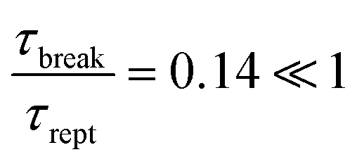 , confirming that the micelles are in the fast-breaking limit where the fluid is well-described by the idealized Maxwell model.75
2.3. Device architecture and fabrication
The serpentine channels used for the flow experiments comprise 19 semi-circular half-loops with inner radius Ri, fixed channel width W = 1 mm, outer radius Ro = Ri + W, fixed channel height H = 2 mm, and fixed aspect ratio H/W = 2; an optical top-down image of a representative example is shown in Fig. 2(a). We choose a large channel aspect ratio to ensure that the dominant velocity gradients arise in the flow imaging plane. All the quantitative results presented in this paper are for channels with Ri = 300 μm; however, as shown in ESI† Movies S3 and S4, we observe similar behavior in channels with Ri = 500 and 1000 μm. | ||
| Fig. 2 Serpentine channel geometry and experimental setup. (a) Brightfield optical image of the serpentine channel device comprised of 19 semi-circular half-loops with inner radius Ri and channel width W. (b) Schematic of experimental setup for flow visualization. | ||
We design the body of each channel [dark blue in Fig. 2(b)] using CAD software (Onshape) and 3D-print it with a clear methacrylate-based polymeric resin (FLGPCL04) using a FormLabs Form 3 stereolithography printer. This resin is inert and likely does not interact with or alter the WLM solution through specific chemical interactions.2,76,77 Moreover, while slight surfactant adsorption to the channel walls may occur, given the device geometry, we estimate that the resulting change in the solution concentration is at most 0.05%—negligible compared to the concentration used in our experiments. We assemble each millifluidic device by screwing together this 3D-printed channel body and a laser-cut transparent acrylic top sheet (McMaster-Carr) [gray in Fig. 2(b)], with a ∼1 mm-thick layer of polydimethylsiloxane (PDMS; Dow SYLGARD 184, 8.5![[thin space (1/6-em)]](https://www.rsc.org/images/entities/char_2009.gif) :1.5 base:curing agent by weight) sandwiched in between to act as a gasket. We then glue flexible Tygon tubing (McMaster-Carr) in the inlet and outlet using a 2-part watertight epoxy (JB MarineWeld).
:1.5 base:curing agent by weight) sandwiched in between to act as a gasket. We then glue flexible Tygon tubing (McMaster-Carr) in the inlet and outlet using a 2-part watertight epoxy (JB MarineWeld).
2.4. Flow imaging
Before each flow experiment, we flush the device to be used with ultrapure Millipore water to remove any residual debris or air bubbles. We then fully saturate the channel with the WLM solution to be tested at a flow rate of 1 mL h−1 for at least 3 h using a syringe pump (Harvard Apparatus PHD 2000). The device is affixed to the stage of an inverted Nikon A1R+ laser scanning confocal fluorescence microscope, ensuring that the syringe pump, device, and outlet waste jar are at the same height to avoid hydrostatic pressure differences, as shown in Fig. 2(b).In each experiment, we impose a stepwise ramp of increasing flow rate Q from 0.5 to 6 mL h−1, allowing the flow to equilibrate at each flow rate for 30 min before commencing imaging. For each flow rate tested, we use a 4× objective lens to acquire 2 min long (∼86 λM) movies at 30 frames per second focused on a horizontal optical plane, 37 μm in thickness, centered at the mid-channel height to avoid boundary effects induced by the top and bottom channel walls. Each movie is taken at each successive half-loop along the length of the serpentine array, with a 3167 × 3167 μm2 field of view at a resolution of 6 μm per pixel. The fluorescent tracer particles seeded in the fluid are excited by a 488 nm laser and their emission is detected using a 500–550 nm sensor.
To characterize the flow behavior, we define a nominal shear rate using the channel half-width W/2 as the characteristic length scale:  . Our experiments probe the range 0.14 ≤ ≤ 1.7 s−1; as shown by the gray region in Fig. 1(a), this range corresponds to strongly shear thinning conditions for the WLM solution. We thereby define the Weissenberg number Wi, which compares the relative strength of elastic and viscous stresses, as
  , where N1() and η() are given by the power law and Carreau–Yasuda fits to the bulk shear rheology, respectively. Our experiments probe the range 0.17 < Wi < 0.78, and the onset of shear thinning arises at Wi0 = Wi(0) = 0.19. For flow conditions exceeding Wi = 0.78, we are unable to obtain PIV measurements for quantitative analysis.
To visualize the WLM solution flow, we generate fluid pathline images and movies using grouped projections of mean pixel intensity over successive frames using the open-source software ImageJ.78,79 Pathlines correspond to trajectories of tracer particles as they are advected by the fluid flow. Example movies are shown in ESI† Movies S1–S4. To quantitatively analyze the flow field, we directly measure each time-resolved 2D velocity field u using PIVlab,80 manually isolating regions in the imaged field of view that only contain fluid flow. We then use the FFT window deformation algorithm with 4 passes of decreasing interrogation area from 64–32–16–16 pixel box sizes and 50% overlap, producing a spatial grid resolution of 50 μm for which particles in each PIV voxel travel approximately 4–8 pixels between successive frames.81,82 Given that the channel width of 1 mm greatly exceeds the spatial PIV resolution, this approach resolves flow gradients in the selected 2D imaging plane. Similarly, the imaging frame rate (30 frames per second) sets the temporal resolution of our velocity fields (33 ms). Given the fluid relaxation time of 1.4 s and total imaging time at each location of 120 s, our approach enables us to resolve temporal variations in the flow field for variations occurring over a broad range of timescales from 33 ms to 120 s. Finally, we use in-house MATLAB codes to process the velocity fields for all analyses. We characterize the flow in each channel using three metrics: the normalized velocity magnitude |u|/max(|u|), root mean square velocity fluctuations  and shear rate
  , where x and t represent the 2D position in the horizontal optical plane and time, respectively, and
  is the rate-of-strain tensor computed from the measured velocity field.
3. Results and discussion
3.1. Base steady laminar flow
We first characterize the steady base flow of the WLM solution in the serpentine channels at low Wi. A representative pathline image of the laminar steady flow at Wi = 0.18 is shown in Fig. 3(a), and the velocity profiles at the apex and exit of a half-loop are shown for the regions outlined in yellow and red in Fig. 3(b), respectively; the corresponding ESI† Movie S1 shows that the pathlines remain unchanging over time. Notably, at the apex of the bend, the velocity profile is highly asymmetric and skewed toward the outer bend. While the curvature of the channel walls is known to induce slight asymmetry in Newtonian flows,61,63,64,83 in this case the velocity profiles are starkly different. In particular, as shown in Fig. 3(b), the flow is plug-like, unlike the typical parabolic profile associated with Poiseuille flow, because of the shear thinning of the WLM solution. Additionally, near the channel walls, the velocity does not decrease to zero—indicating strong slip caused by shear localization at the fluid–solid boundary, as has been reported for WLM flows in other geometries.17,26,66,69 We estimate characteristic slip velocities by linearly extrapolating the velocity profiles near the solid surfaces, finding average slip velocities of 0.07, 0.22, and 0.48 mm s−1 at flow rates Q = 0.5, 1.5, and 3 mL h−1, respectively, indicating that the extent of slip increases monotonically with increasing flow rate in the steady flow regime. The corresponding slip lengths (>100 μm in all cases) greatly exceed the spatial resolution of PIV (50 μm), which additionally confirms the presence of strong slip. The estimated slip velocities are persistent in time in the steady flow regime, indicating sustained shear localization occurring at the channel walls. | ||
| Fig. 3 Base steady laminar flow exhibits strong shear thinning and slip at surfaces. (a) Pathline image of flow in the Ri = 300 μm device at Wi = 0.18 < Wic, generated using a moving average of fluorescence intensity over 60 frames. Scale bar is 500 μm. (b) Time-averaged (over 86λ) velocity profiles, normalized by the maximum velocity, at the apex (yellow rectangle) and end (red rectangle) of a half-loop. All velocity profiles exhibit highly asymmetric plug flow and indicate the presence of a substantial slip velocity at surfaces. The PIV grid resolution used is 0.05 W. (c) Streamline visualization and color maps of the normalized velocity magnitudes at selected half-loop locations further reflect strong plug flow and asymmetry in the base laminar flow state. | ||
Interestingly, we observe hints of shear inhomogeneity reminiscent of shear banding behavior—referred to here as “shear localization”—when Wi is increased slightly to 0.25, as shown by the inflection in the blue profile shown in the right-hand plot of Fig. 3(b). This effect diminishes upon further increasing Wi, as shown by the green profile in Fig. 3(b), suggesting that the flow re-homogenizes across the channel width. A representative image showing the velocity magnitudes and flow streamlines across multiple half-loops is shown in Fig. 3(c) for this case of Wi = 0.43, at which the flow remains laminar and steady. The analyses in Fig. 3 present 2D velocity profiles measured at the channel mid-plane; however, due to the 3D nature of the channel, steady secondary flows not captured by our 2D measurement likely arise due to the inversion of curvature in the serpentine geometry, as have been reported previously.83–86
3.2. Onset of 3D unsteady flow
Further increasing Wi gives rise to an elastic flow instability where this base steady flow becomes unstable to 3D unsteady flow. An example is shown in Fig. 4(a); for this channel geometry, the onset of the instability—determined as when the rms velocity fluctuations exceed a threshold value of 0.2 set by the noise threshold of the PIV measurements—occurs at a critical value Wi = Wic ≈ 0.7. Such purely-elastic instabilities are typically generated through the coupling of elastic normal stresses and streamline curvature, which gives rise to destabilizing hoop stresses.34,36–38 This coupling can also be described using a dimensionless parameter developed by Pakdel and McKinley:36,37 , where U = Q/(HW) is the average flow velocity. In our experiments, the critical value of M = Mc ≈ 2.5, in good agreement with prior measurements across a broad range of fluids and geometries.38
 | ||
Fig. 4 Unsteady 3D flow arising from an elastic instability. (a) Color maps of the flow field measured at the channel mid-height in the unsteady flow state showing the (top) normalized velocity magnitude |u|/max(|u|), (middle) root-mean-square (rms) velocity magnitude fluctuations  and (bottom) shear rate (x) in the Ri = 300 μm channel at Wi = 0.78 > Wic. The top and bottom rows show near-instantaneous flow fields that are time-averaged over a duration of 1 λM to reduce noise. The middle row shows rms velocity fluctuations over a duration of 86 λM, highlighting the spatial heterogeneity and temporal persistence of flow fluctuations. All color maps comprise stitched fields-of-view obtained sequentially during flow imaging, giving rise to the visible discontinuities between adjacent half-loops. (b) Power spectral densities of the magnitude of velocity fluctuations indicate that above the onset of the elastic instability, more energy is dissipated in fluctuations across a broad range of frequencies, with no characteristic time scale. and (bottom) shear rate (x) in the Ri = 300 μm channel at Wi = 0.78 > Wic. The top and bottom rows show near-instantaneous flow fields that are time-averaged over a duration of 1 λM to reduce noise. The middle row shows rms velocity fluctuations over a duration of 86 λM, highlighting the spatial heterogeneity and temporal persistence of flow fluctuations. All color maps comprise stitched fields-of-view obtained sequentially during flow imaging, giving rise to the visible discontinuities between adjacent half-loops. (b) Power spectral densities of the magnitude of velocity fluctuations indicate that above the onset of the elastic instability, more energy is dissipated in fluctuations across a broad range of frequencies, with no characteristic time scale. | ||
As shown by the maps in Fig. 4(a), all three flow metrics exhibit pronounced heterogeneity throughout the channel. To further characterize the flow dynamics, we examine the temporal power spectral density (PSD) of the magnitude of velocity fluctuations across different frequencies f:  , where L is the duration of the signal, Fs is the sampling rate, and FFT denotes a fast Fourier transform. Our results, spatially averaged over all PIV voxels, are shown in Fig. 4(b). Above the onset of the elastic instability, the PSD exhibits a broad power law decay E(f) ∼ f−α, with α ≈ 2.6 at Wi = 0.78, reflecting energy dissipation by flow fluctuations across a broad range of time scales—consistent with previous characterizations of polymeric and WLM elastic instabilities in other confined geometries.26,30,39,45,46,63,64,87–89 The absence of distinct peaks in the PSD indicates that the unsteady flow is aperiodic with no characteristic time scales. Analysis of the instantaneous velocity profiles shows the presence of pronounced slip behavior consistent with the strong slip present in the steady flow regime (Section 3.1); however, the estimated slip velocities now vary greatly over time (e.g. ranging from 0 to 2.54 mm s−1 at Q = 6 mL h−1) due to the strongly fluctuating nature of the flow.
≈ 0 s−1) and the flowing regions, generating a strong shear rate gradient at the dead zone boundary; by contrast, if the fluid could not support shear localization, dead zones would not form, as previously documented for non-shear banding elastic polymer solutions.61–64
 | ||
| Fig. 5 Characterization of dead zone formation, dynamics, and size. (a) Temporal evolution of shear rate profiles along the channel width (location shown in inset). Successive curves are plotted at time intervals of 6.7 s. At early times (0 < t < 90 s), a large peak in shear rate separates the dead zone ( ≈ 0 s−1) from the bulk flow, while at later times the dead zone is washed away and the shear rate profile re-homogenizes. (b) Example instantaneous pathline image of the unsteady flow state in a selected half-loop. Yellow dashed lines demarcate example dead zone regions. Scale bar shows 500 μm. (c) Temporal variation of dead zone size ADZ in selected half-loops shows considerable fluctuations. The shaded gray region denotes the range of theoretically-predicted dead zone areas from considering minimization of local streamline curvature. (d) Power spectral densities of dead zone size fluctuations indicate no characteristic time scale. (e) Probability density distribution of normalized dead zone areas ADZ/Ahalfloop with increasing advective Deborah number Deadv shows a broad increase in dead zone sizes for Deadv > 1. (f) Degree of multistability ξ describing the range of observed dead zone sizes at a given flow condition shows onset of multistable dead zone behavior above Deadv = 1. All data in (a)–(d) are for Wi = 0.78. | ||
To characterize their dynamics, we track variations in the dead zone areas (ADZ) over time. Examples for selected half loops along the length of the channel are shown by the traces in Fig. 5(c). Notably, the dead zone sizes fluctuate dramatically over time, often persisting over durations much longer than the characteristic relaxation time λM = 1.4 s. These fluctuations do not have any clear periodicity; instead, they mirror the spectrum of bulk velocity fluctuations shown in Fig. 4(b), as reflected by the broad decay in the power spectral density EDZ(f) in Fig. 5(d)—indicating that dead zone fluctuations are established by the unstable fluctuations in the freely-flowing fluid outside the dead zone. Despite these fluctuations, however, all dead zones are bounded by a maximal size AmaxDZ, indicated by the gray region in Fig. 5(c).
Intriguingly, for a given unstable flow rate and at a given time, not all half-loops contain dead zones—as shown in Fig. 4(a) and 5(c). Instead, they exhibit multistable behavior: some half-loops do not have dead zones (the dead zone-free state), while other half-loops have persistent dead zones of varying sizes (the dead zone-containing state). As time progresses, a given half-loop can randomly switch from the dead zone-free state to the dead zone-containing state and vice versa; an example is shown by the different traces in Fig. 5(a), in which a dead zone eventually washes away, as well as those in Fig. 5(c). This behavior is reminiscent of the multistability exhibited by eddies during the unstable flow of elastic polymer solutions in pore constriction arrays,90–92 in which multistability arises when flow-induced elastic stresses do not have sufficient time to relax as they are advected between constrictions. Hence, following this prior work, we parameterize the onset of the multistability observed for WLM solutions in serpentine channels using a streamwise Deborah number comparing the stress relaxation time of the WLM solution to the time required for the fluid to be advected between adjacent half-loops:  where tadv = HAhalfloop/Q and Ahalfloop is the half-loop area. Consistent with this prior work, we also find that multistability arises when Deadv ≳ 1. For example, Fig. 5(e) shows a color map of the probability density function (p.d.f.) of the dead zone areas aggregated over the different half-loops, normalized by Ahalfloop, for the different Deadv tested—showing that this p.d.f. abruptly begins to broaden, a hallmark of multistability, when Deadv ≳ 1. Furthermore, also following prior work, we define the degree of multistability
  , where ξ = 0 indicates no multistable behavior and ξ = 1 describes the maximum possible extent of multistable behavior. As shown in Fig. 5(f), we again see an abrupt increase in the degree of multistability ξ when Deadv ≳ 1. Taken together, these results demonstrate that fluid elasticity plays a key role in determining dead zone formation.
Motivated by these findings, as well as previous work describing the shapes of eddies formed in elastic polymer solutions entering contractions,93–97 we conjecture that considering the elastic stresses generated during WLM solution flow in a serpentine channel can help predict the maximal dead zone size AmaxDZ. In particular, given that these elastic hoop stresses are generated by streamline curvature,36,37 we expect that the interface between a dead zone and the surrounding freely-flowing region forms to minimize local streamline curvature. This idea can be formulated using a simple geometric description (detailed in the Appendix): for a given half-loop, we expect that the largest dead zone that can form in a half-loop is bounded by a straight line tangent to the inner bend of the loop, as shown in Fig. 7. This prediction, shown by the gray shaded region in Fig. 5(c), agrees reasonably well with the experimental measurements as an upper bound AmaxDZ to the individual traces of ADZ.
 | ||
| Fig. 6 3D twisting flows intermittently arise in the unsteady flow. (a) Snapshots of the velocity field (arrows) superimposed on a color map of normalized velocity magnitude at different times, showing a representative twisting event. (b) Probability density function of the divergence of the measured 2D flow field suggests an increase in 3D flow above the onset of instability (Wi > Wic ≈ 0.7). (c) Twisting reduces the hydrodynamic tortuosity of fluid streamlines: the blue dashed curve is the center semi-circular streamline in the base flow, and the green dashed curve is the projected 2D sinusoidal path enabled by 3D twisting. Pathline images are generated using a moving average of fluorescence intensity over 10 frames. Scale bar is 500 μm. Data in (a) and (c) are for Wi = 0.78. | ||
 | ||
| Fig. 7 Schematic describing the geometric prediction of dead zone size and shape in the serpentine channels. | ||
 , using the in-plane velocity components. Under steady flow conditions (Wi = 0.18–0.43), the 2D divergence is close to zero, with slight deviations due to small weakly-3D secondary flows generated by the inversion of curvature at corners and bends;83–86 however, in the unstable flow state (Wi = 0.78), an appreciable fraction of the 2D divergence becomes non-zero, reflecting flow in the third dimension.
Despite their complexity, we attempt to rationalize the basic geometric properties of these 3D inversion events by again considering minimization of the local streamline curvature—which here manifests as a reduction of the 2D hydrodynamic tortuosity, τ. In the base laminar flow, the streamlines can be approximated as a semi-circular path shown by the blue dashed line in Fig. 6(c); the associated tortuosity, given by the ratio of the total path length to the horizontal streamwise distance traveled, is then  . Guided by the visualization in ESI† Movie S4 and Fig. 6(a), we approximate the “disclination” boundary of the twisting flow as a periodic sinusoidal function with amplitude Ri and period 2(Ri + Ro). As shown by the green dashed line in Fig. 6(c), this approximation is in good agreement with the experimental observations. The resulting 2D hydrodynamic tortuosity is then given by
  , where x and y represent the streamwise and transverse position coordinates. For this channel, this calculation then yields a tortuosity of 1.08, representing a 31% reduction from the laminar base case.
4. Conclusions
In this study, we investigated the flow behavior of a highly elastic, shear thinning, semi-dilute WLM solution in serpentine channels at low Reynolds number (Re ≪ 1) and moderate Weissenberg numbers (Wi ∼ 1). The serpentine microchannels are composed of successive semi-circular half-loops, thereby enabling us to experimentally isolate the influence of streamline curvature—a fundamental feature of many real-world flows—on the flow behavior without being confounded by other geometric complexities. Our flow visualization experiments revealed three key phenomena:1. At low Wi, the base flow is steady and laminar but exhibits spatial asymmetry with wall slip, reflecting the shear thinning and shear localization tendencies of the WLM solution. Above a critical Wi = Wic ≈ 0.7, the flow undergoes an elastic instability and transitions to a 3D unsteady flow state characterized by pronounced spatiotemporal velocity fluctuations. This transition occurs at a critical Pakdel–McKinley parameter value of Mc ≈ 2.5, consistent with other measurements across different viscoelastic fluids and geometries.
2. Alongside this unstable bulk flow, dead zones of stagnant fluid form in the downstream portion of half-loops—reflecting the ability of the WLM solution to support shear localization, complementing reports of dead zone formation for other types of complex fluids.98–102 Due to coupling to the velocity fluctuations in the bulk flow, these dead zones fluctuate in their size; however, they are bounded by a maximal size that minimizes the fluid streamline curvature, and therefore the generation of elastic stresses. Dead zones also exhibit multistable behavior—forming and persisting in some half-loops, not forming in other half-loops, and randomly switching between these two states. This multistability arises when the advective Deborah number Deadv ≳ 1, indicating that it occurs because elastic stresses generated by fluid flow do not have sufficient time to relax between consecutive half-loops. This finding expands on previous studies of multistability, which were restricted to elastic polymer solutions flowing through pore constriction arrays,90–92 to a broader range of fluids and flow geometries.
3. The unstable flow state also features intermittent, 3D “twisting” velocity inversion events amid the spatiotemporally-fluctuating bulk flow. These twisting events reduce the hydrodynamic tortuosity compared to the base flow state, and their geometric structure can also be rationalized as minimizing the fluid streamline curvature, and therefore the generation of elastic stresses.
These findings highlight how the shear localization and elastic properties of WLM solutions give rise to unusual flow behaviors in tortuous channels, expanding current understanding of complex fluid flows in complex geometries. Further investigating the physics underlying the formation of the dead zones and 3D twisting events revealed by our experiments will be a useful direction for future work.
Several extensions of our study offer opportunities for future research. While our imaging focused on a single optical plane at the mid-channel height, full 3D velocimetry in channels of varying aspect ratio (H/W) would provide more comprehensive insights into the nature of the 3D twisting events we observed. Furthermore, direct measurements of the stress field during flow could provide deeper insights into the coupling between elastic stresses and flow structures (e.g., dead zones, 3D twisting events). Our experiments probed a wide range of shear rates, but they all fell on the stress plateau measured in the bulk shear rheology shown in Fig. 1(a); exploring a wider range of shear rates below and above this plateau will help further elucidate WLM flow dynamics across a broader range of conditions.
Finally, while here we focused on a single semi-dilute, linear, entangled WLM solution, future studies could explore other formulations with different rheological properties (e.g., varying the degrees of shear thinning and elasticity by tuning the molar ratio of surfactant to salt). Studies could also probe how variations in the micellar microstructure67,70,103,104 influence the flow behavior—which could potentially guide ways to use stimulus-responsive WLMs10,18 to achieve targeted local flow behaviors. For example, controllably forming stagnant dead zones could be a mechanism to redirect flow on demand, while conversely, prevention of dead zone formation could help promote fluid homogenization.
Author contributions
E. Y. C.: conceptualization, methodology, investigation, formal analysis, writing; S. S. D.: conceptualization, resources, supervision, writing.Data availability
The data that support the findings of this study are available within the article. Supplementary movies are available online at https://github.com/emchen6639/WLMserpentine.Conflicts of interest
There are no conflicts to declare.Appendix
Geometric prediction of dead zone shape and size
For one unit cell of the serpentine geometry, the upper boundary can be described aswhere x and y represent the streamwise and transverse position coordinates. Similarly, the bottom boundary can be described as


Given a selected fixed point (xb, yb) on the outer boundary of a half loop, as depicted in Fig. 7, we seek to determine the location on the following inner bend (x*, y*) such that the line between the two points is tangent to the inner half-loop boundary, thereby minimizing local streamline curvature. The slope between the two points is  , which is equal to the derivative of inner curve parameterization evaluated at (x*, y*):
  . Further, the point (x*, y*) must lie on both the inner curve equation and the tangent line equation. Accordingly, (x*, y*) is straightforwardly determined from the solution of:

Note that only one of two solutions is physical in the context of our experiments. By varying the selected point (xb, yb), we obtain predictions of the dead zone shape and size where the dead zone is bounded by the resulting tangent line and the outer channel boundary. Example solutions are shown by the red lines in Fig. 7. The maximum dead zone size is set by the physical constraints of the bounding geometry as conservation of mass requires that some finite region of the channel must contain non-zero flow velocity. The resulting range of theoretical dead zone size predictions 0 ≤ ApredDZ ≤ AmaxDZ is given by the shaded region in Fig. 5(c) and is in good agreement with the experimentally-measured values of dead zone sizes.
Acknowledgements
We acknowledge support from the Princeton Center for Complex Materials (PCCM), a National Science Foundation (NSF) Materials Research Science and Engineering Center (MRSEC; DMR-2011750), as well as the Camille Dreyfus Teacher-Scholar Program of the Camille and Henry Dreyfus Foundation. We also acknowledge the use of the Imaging and Analysis Center (IAC) operated by the Princeton Materials Institute at Princeton University. It is a pleasure to thank Howard Stone for useful feedback.References
- R. G. Larson, The Structure and Rheology of Complex Fluids, Oxford University Press, 1999 Search PubMed.
- C. A. Dreiss, Wormlike Micelles: Advances in Systems, Characterisation and Applications, The Royal Society of Chemistry, 2017, pp. 1–8 Search PubMed.
- B. Chase, W. Chmilowski, R. Marcinew, C. Mitchell and Y. Dang, Oilfield Rev., 1997, 9, 20–33 CAS.
- R. Zana and E. W. Kaler, Giant Micelles Properties and Applications, CRC Press, Boca Raton, 1st edn, 2007 Search PubMed.
- E. Jafari Nodoushan, T. Yi, Y. J. Lee and N. Kim, Fluids, 2019, 4, 173 CrossRef.
- A. Du, C. Ye, J. Chen, F. Sun and J. Mao, Colloids Surf., A, 2023, 672, 131707 CrossRef CAS.
- J.-H. Kwon, M.-K. Ji, R. Kumar, M. M. Islam, M. A. Khan, Y.-K. Park, K. K. Yadav, R. Vaziri, J.-H. Hwang, W. H. Lee, Y.-T. Ahn and B.-H. Jeon, Rev. Environ. Sci. Biotechnol., 2023, 22, 679–714 CrossRef CAS.
- D. B. Tripathy, ACS EST Water, 2024, 4, 4721–4740 CrossRef CAS.
- K. Gasljevic and E. Matthys, Energy Build., 1993, 20, 45–56 Search PubMed.
- H. Shi, W. Ge, H. Oh, S. M. Pattison, J. T. Huggins, Y. Talmon, D. J. Hart, S. R. Raghavan and J. L. Zakin, Langmuir, 2013, 29, 102–109 Search PubMed.
- M. Kotenko, H. Oskarsson, C. Bojesen and M. P. Nielsen, Energy, 2019, 178, 72–78 CrossRef.
- G. Rose and K. Foster, J. Non-Newtonian Fluid Mech., 1989, 31, 59–85 CrossRef CAS.
- K. Gasljevic, G. Aguilar and E. Matthys, J. Non-Newtonian Fluid Mech., 2001, 96, 405–425 CrossRef CAS.
- J. Yang, Curr. Opin. Colloid Interface Sci., 2002, 7, 276–281 CrossRef CAS.
- R. K. Rodrigues, L. A. S. Silva, G. G. Vargas and B. V. Loureiro, J. Surfactants Deterg., 2020, 23, 21–40 Search PubMed.
- R. S. Mitishita, G. J. Elfring and I. A. Frigaard, J. Non-Newtonian Fluid Mech., 2022, 301, 104724 CrossRef CAS.
- R. R. Gupta, M. Daneshi, I. Frigaard and G. Elfring, Soft. Matter., 2024, 20, 4715–4733 RSC.
- Z. Chu, C. A. Dreiss and Y. Feng, Chem. Soc. Rev., 2013, 42, 7174–7203 Search PubMed.
- H. Yu, Z. Xu, D. Wang, X. Chen, Z. Zhang, Q. Yin and Y. Li, Polym. Chem., 2013, 4, 5052 RSC.
- C. Lim, J. D. Ramsey, D. Hwang, S. C. M. Teixeira, C. Poon, J. D. Strauss, E. P. Rosen, M. Sokolsky-Papkov and A. V. Kabanov, Small, 2022, 18, 2103552 Search PubMed.
- W. Hartt, L. Bacca and E. Tozzi, Soft Matter Series, Royal Society of Chemistry, Cambridge, 2017, pp. 379–398 Search PubMed.
- F. Choi, R. Chen and E. J. Acosta, J. Colloid Interface Sci., 2020, 564, 216–229 CrossRef CAS PubMed.
- J.-B. Salmon, A. Colin, S. Manneville and F. Molino, Phys. Rev. Lett., 2003, 90, 228303 CrossRef PubMed.
- S. Lerouge and J.-F. Berret, Polymer Characterization, Springer Berlin Heidelberg, Berlin, Heidelberg, 2009, vol. 230, pp. 1–71 Search PubMed.
- S. M. Fielding and H. J. Wilson, J. Non-Newtonian Fluid Mech., 2010, 165, 196–202 Search PubMed.
- M. A. Fardin and S. Lerouge, Eur. Phys. J. E: Soft Matter Biol. Phys., 2012, 35, 91 CrossRef PubMed.
- T. Divoux, M. A. Fardin, S. Manneville and S. Lerouge, Annu. Rev. Fluid Mech., 2016, 48, 81–103 CrossRef.
- P. Rassolov, A. Scigliani and H. Mohammadigoushki, Soft. Matter., 2017, 13, 8368–8378 RSC.
- L. Bécu, D. Anache, S. Manneville and A. Colin, Phys. Rev. E: Stat., Nonlinear, Soft Matter Phys., 2007, 76, 011503 Search PubMed.
- M. A. Fardin, D. Lopez, J. Croso, G. Grégoire, O. Cardoso, G. H. McKinley and S. Lerouge, Phys. Rev. Lett., 2010, 104, 178303 Search PubMed.
- M. A. Fardin, T. J. Ober, C. Gay, G. Grégoire, G. H. McKinley and S. Lerouge, EPL, 2011, 96, 44004 CrossRef.
- J. Beaumont, N. Louvet, T. Divoux, M.-A. Fardin, H. Bodiguel, S. Lerouge, S. Manneville and A. Colin, Soft. Matter., 2013, 9, 735–749 RSC.
- S. M. Fielding, J. Rheol., 2016, 60, 821–834 CrossRef CAS.
- R. G. Larson, E. S. G. Shaqfeh and S. J. Muller, J. Fluid Mech., 1990, 218, 573–600 CrossRef CAS.
- R. Larson, S. Muller and E. Shaqfeh, J. Non-Newtonian Fluid Mech., 1994, 51, 195–225 CrossRef CAS.
- P. Pakdel and G. H. McKinley, Phys. Rev. Lett., 1996, 77, 2459–2462 CrossRef CAS PubMed.
- G. H. McKinley, P. Pakdel and A. Öztekin, J. Non-Newtonian Fluid Mech., 1996, 67, 19–47 CrossRef CAS.
- S. S. Datta, A. M. Ardekani, P. E. Arratia, A. N. Beris, I. Bischofberger, G. H. McKinley, J. G. Eggers, J. E. López-Aguilar, S. M. Fielding, A. Frishman, M. D. Graham, J. S. Guasto, S. J. Haward, A. Q. Shen, S. Hormozi, A. Morozov, R. J. Poole, V. Shankar, E. S. G. Shaqfeh, H. Stark, V. Steinberg, G. Subramanian and H. A. Stone, Phys. Rev. Fluids, 2022, 7, 080701 CrossRef.
- C. A. Browne and S. S. Datta, Sci. Adv., 2021, 7, eabj2619 CrossRef CAS PubMed.
- C. A. Browne and S. S. Datta, Proc. Natl. Acad. Sci. U. S. A., 2024, 121, e2320962121 CrossRef CAS PubMed.
- P. F. Salipante, C. A. E. Little and S. D. Hudson, Phys. Rev. Fluids, 2017, 2, 033302 CrossRef PubMed.
- S. J. Haward, F. J. Galindo-Rosales, P. Ballesta and M. A. Alves, Appl. Phys. Lett., 2014, 104, 124101 CrossRef.
- M. Y. Hwang, H. Mohammadigoushki and S. J. Muller, Phys. Rev. Fluids, 2017, 2, 043303 CrossRef.
- Y. Zhang, H. Mohammadigoushki, M. Y. Hwang and S. J. Muller, Phys. Rev. Fluids, 2018, 3, 093301 CrossRef.
- P. F. Salipante, S. E. Meek and S. D. Hudson, Soft. Matter., 2018, 14, 9020–9035 RSC.
- R. M. Matos, M. A. Alves and F. T. Pinho, Exp. Fluids, 2019, 60, 145 CrossRef.
- F. Hillebrand, S. Varchanis, C. C. Hopkins, S. J. Haward and A. Q. Shen, Soft. Matter., 2024, 20, 7133–7146 RSC.
- G. R. Moss and J. P. Rothstein, J. Non-Newtonian Fluid Mech., 2010, 165, 1505–1515 CrossRef CAS.
- S. J. Haward, N. Kitajima, K. Toda-Peters, T. Takahashi and A. Q. Shen, Soft. Matter., 2019, 15, 1927–1941 RSC.
- C. C. Hopkins, S. J. Haward and A. Q. Shen, Small, 2020, 16, 1903872 CrossRef CAS PubMed.
- C. Hopkins, A. Shen and S. Haward, Soft. Matter., 2022, 18, 8856–8866 RSC.
- C. Hopkins, S. Haward and A. Shen, Soft. Matter., 2022, 18, 4868–4880 RSC.
- S. Chen and J. P. Rothstein, J. Non-Newtonian Fluid Mech., 2004, 116, 205–234 CrossRef CAS.
- S. Wu and H. Mohammadigoushki, J. Rheol., 2018, 62, 1061–1069 CrossRef CAS.
- S. Wu and H. Mohammadigoushki, Soft. Matter., 2021, 17, 4395–4406 RSC.
- G. R. Moss and J. P. Rothstein, J. Non-Newtonian Fluid Mech., 2010, 165, 1–13 CrossRef CAS.
- S. De, S. P. Koesen, R. V. Maitri, M. Golombok, J. T. Padding and J. F. M. van Santvoort, AIChE J., 2018, 64, 773–781 CrossRef CAS.
- S. J. Haward, C. C. Hopkins and A. Q. Shen, Proc. Natl. Acad. Sci. U. S. A., 2021, 118, e2111651118 CrossRef CAS PubMed.
- A. Groisman and V. Steinberg, Nature, 2001, 410, 905–908 CrossRef CAS PubMed.
- T. Burghelea, E. Segre, I. Bar-Joseph, A. Groisman and V. Steinberg, Phys. Rev. E: Stat., Nonlinear, Soft Matter Phys., 2004, 69, 066305 CrossRef PubMed.
- J. Zilz, R. J. Poole, M. A. Alves, D. Bartolo, B. Levaché and A. Lindner, J. Fluid Mech., 2012, 712, 203–218 CrossRef CAS.
- L. Casanellas, M. Alves, R. Poole, S. Lerouge and A. Lindner, Soft. Matter., 2016, 12, 6167–6175 RSC.
- A. Souliès, J. Aubril, C. Castelain and T. Burghelea, Phys. Fluids, 2017, 29, 083102 CrossRef.
- P. Shakeri, M. Jung and R. Seemann, Phys. Fluids, 2022, 34, 073112 CrossRef CAS.
- H. Rehage and H. Hoffmann, J. Phys. Chem., 1988, 92, 4712–4719 CrossRef CAS.
- R. W. Mair and P. T. Callaghan, Europhys. Lett., 1996, 36, 719–724 Search PubMed.
- C. Oelschlaeger, M. Schopferer, F. Scheffold and N. Willenbacher, Langmuir, 2009, 25, 716–723 Search PubMed.
- S. J. Haward and G. H. McKinley, Phys. Rev. E: Stat., Nonlinear, Soft Matter Phys., 2012, 85, 031502 CrossRef PubMed.
- S. J. Haward, T. J. Ober, M. S. Oliveira, M. A. Alves and G. H. McKinley, Soft. Matter., 2012, 8, 536–555 RSC.
- D. Gaudino, R. Pasquino and N. Grizzuti, J. Rheol., 2015, 59, 1363–1375 CrossRef CAS.
- C. W. Macosko, Rheology: principles, measurements, and applications, VCH, New York, 1994 Search PubMed.
- Y. Zhao, A. Shen and S. Haward, Soft. Matter., 2016, 12, 8666–8681 RSC.
- R. G. Larson, J. Rheol., 2012, 56, 1363–1374 CrossRef CAS.
- R. Granek and M. E. Cates, J. Chem. Phys., 1992, 96, 4758–4767 Search PubMed.
- M. S. Turner and M. E. Cates, Langmuir, 1991, 7, 1590–1594 CrossRef CAS.
- Y. Zhao, P. Cheung and A. Q. Shen, Adv. Colloid Interface Sci., 2014, 211, 34–46 Search PubMed.
- J. P. Rothstein and H. Mohammadigoushki, J. Non-Newtonian Fluid Mech., 2020, 285, 104382 CrossRef CAS.
- M. D. Abràmoff, P. J. Magalhães and S. J. Ram, Biophotonics Intern., 2004, 11, 36–42 Search PubMed.
- J. Schindelin, I. Arganda-Carreras, E. Frise, V. Kaynig, M. Longair, T. Pietzsch, S. Preibisch, C. Rueden, S. Saalfeld, B. Schmid, J.-Y. Tinevez, D. J. White, V. Hartenstein, K. Eliceiri, P. Tomancak and A. Cardona, Nat. Methods, 2012, 9, 676–682 CrossRef CAS PubMed.
- W. Thielicke and E. J. Stamhuis, J. Open Res. Softw., 2014, 2, e30 Search PubMed.
- R. J. Adrian and J. Westerweel, Particle Image Velocimetry, Cambridge University Press, New York, 2011 Search PubMed.
- M. Raffel, C. E. Willert, F. Scarano, C. J. Kähler, S. T. Wereley and J. Kompenhans, Particle Image Velocimetry: A Practical Guide, Springer, Switzerland, 2018 Search PubMed.
- L. Ducloué, L. Casanellas, S. Haward, R. Poole, M. Alves, S. Lerouge, A. Shen and A. Lindner, Microfluid. Nanofluid., 2019, 23, 33 CrossRef.
- R. Rusconi, S. Lecuyer, N. Autrusson, L. Guglielmini and H. Stone, Biophys. J., 2011, 100, 1392–1399 CrossRef CAS PubMed.
- R. Poole, A. Lindner and M. Alves, J. Non-Newtonian Fluid Mech., 2013, 201, 10–16 Search PubMed.
- M. K. Kim, K. Drescher, O. Shun Pak, B. L. Bassler and H. A. Stone, New J. Phys., 2014, 16, 065024 CrossRef PubMed.
- A. Groisman and V. Steinberg, New J. Phys., 2004, 6, 29 CrossRef.
- D. W. Carlson, K. Toda-Peters, A. Q. Shen and S. J. Haward, J. Fluid Mech., 2022, 950, A36 CrossRef CAS.
- E. Y. Chen, C. A. Browne, S. J. Haward, A. Q. Shen and S. S. Datta, Stagnation points at grain contacts generate an elastic flow instability in 3D porous media, arXiv, 2024, preprint, arXiv:2412.03510 [physics] DOI:10.48550/arXiv.2412.03510,https://arxiv.org/abs/2412.03510.
- C. Browne, A. Shih and S. Datta, J. Fluid Mech., 2020, 890, A2 CrossRef CAS.
- M. Kumar, S. Aramideh, C. A. Browne, S. S. Datta and A. M. Ardekani, Phys. Rev. Fluids, 2021, 6, 033304 CrossRef.
- E. Y. Chen and S. S. Datta, J. Rheol., 2025, 69, 235–249 CrossRef CAS.
- G. K. Batchelor, J. Fluid Mech., 1971, 46, 813–829 CrossRef.
- D. V. Boger, Annu. Rev. Fluid Mech., 1987, 19, 157–182 CrossRef.
- A. Mongruel and M. Cloitre, Phys. Fluids, 1995, 7, 2546–2552 Search PubMed.
- A. Mongruel and M. Cloitre, J. Non-Newtonian Fluid Mech., 2003, 110, 27–43 Search PubMed.
- L. Rodd, J. Cooper-White, D. Boger and G. McKinley, J. Non-Newtonian Fluid Mech., 2007, 143, 170–191 CrossRef CAS.
- P. Coussot, J. Non-Newtonian Fluid Mech., 2014, 211, 31–49 CrossRef CAS.
- N. Waisbord, N. Stoop, D. M. Walkama, J. Dunkel and J. S. Guasto, Phys. Rev. Fluids, 2019, 4, 063303 CrossRef.
- M. S. Abdelgawad, S. J. Haward, A. Q. Shen and M. E. Rosti, Phys. Fluids, 2024, 36, 113127 CrossRef CAS.
- D. Kawale, G. Bouwman, S. Sachdev, P. L. J. Zitha, M. T. Kreutzer, W. R. Rossen and P. E. Boukany, Soft. Matter., 2017, 13, 8745–8755 Search PubMed.
- Y. Ichikawa and M. Motosuke, Microfluid. Nanofluid., 2022, 26, 44 CrossRef CAS.
- M. Chellamuthu and J. P. Rothstein, J. Rheol., 2008, 52, 865–884 CrossRef CAS.
- S. A. Rogers, M. A. Calabrese and N. J. Wagner, Curr. Opin. Colloid Interface Sci., 2014, 19, 530–535 CrossRef CAS.
Footnote |
| † Electronic supplementary information (ESI) available: Movie S1. Steady laminar base flow in the Ri = 300 μm channel at Wi = 0.18 < Wic. Successive half-loops are imaged with a time offset of 2 min. Scale bar is 500 μm. Movies play at 3.3× real time and are generated using a moving average of fluorescence intensity over 30 frames. Movie S2. Strongly 3D unsteady flow in the Ri = 300 μm channel at Wi = 0.78 > Wic. Successive half-loops have a time offset of 2 min. Scale bar is 500 μm. Movies play at 3.3× real time and are generated using a moving average of fluorescence intensity over 30 frames. Movie S3. Dead zones arise in the unsteady flow regime in serpentine channels of varied radii of curvature: Ri = 300, 500, and 1000 μm channels, from left to right. Flow is from left to right. Scale bar is 500 μm. Movies play at 3.3× real time and are generated using a moving average of fluorescence intensity over 30 frames. Movie S4. 3D twisting events arise in the unsteady flow regime in serpentine channels of varied radii of curvature: Ri = 300, 500, and 1000 μm channels, from left to right. Flow is from left to right. Scale bar is 500 μm. Movies play at 3.3× real time and are generated using a moving average of fluorescence intensity over 30 frames. See DOI: https://doi.org/10.1039/d5sm00344j |
| This journal is © The Royal Society of Chemistry 2025 |