 Open Access Article
General component additivity, reaction engineering, and machine learning models for hydrothermal liquefaction†
Peter M.
Guirguis
 and
Phillip E.
Savage
 *
*
Chemical Engineering Department, Pennsylvania State University, 121D CBEB Building, University Park, PA 16802, USA. E-mail: psavage@psu.edu
First published on 21st February 2025
Abstract
Hydrothermal liquefaction (HTL) is the process of breaking down renewable biomass resources in hot compressed water to produce crude bio-oil. There are more than a thousand experimental biocrude yields in the literature. We use this extensive data set to parameterize new models for HTL. These new models are general in that they can handle any biomass feedstock and HTL at any set of reaction conditions. We report new component additivity, reaction engineering, and machine learning models that correlate the experimental data and predict biocrude yields with a median absolute residual of no more than 6.3 wt%. These new models predict literature biocrude yields more accurately than any of the previously published models for HTL of biomass. The new component additivity model employs coefficients that are continuous functions of reaction severity and biomass loading (wt%). The new reaction engineering model includes the possibility of portions of the initial feedstock (e.g., lipids) being in one of the product fractions (e.g., biocrude) at t = 0. The decision tree model provided the best fit of the biocrude yields, but it also had far more parameters than did the other models. The component additivity model was superior to the reaction engineering model in fitting the HTL biocrude yields. However, the reaction engineering model is statistically better than the component additivity model at predicting biocrude yields. We use the new models to identify HTL reaction conditions that would maximize yields of biocrude for different types of biomass yet to be investigated experimentally.
Sustainability spotlightHydrothermal liquefaction (HTL) provides a sustainable route to convert wet biomass into renewable biocrude oil, addressing the global need for cleaner energy. This work advances sustainability by creating predictive models that optimize HTL efficiency across varied feedstocks, reducing resource waste and enhancing biofuel viability. By leveraging a large dataset and innovative modeling approaches, this study supports UN SDGs 7 (Affordable and Clean Energy) and 12 (Responsible Consumption and Production), offering tools for better process design, economic assessments, and environmental impact reduction in biofuel production. |
1 Introduction
Hydrothermal liquefaction (HTL) converts renewable wet biomass into biocrude oil via thermochemical processing around 150–600 °C, 30 seconds to 1.5 hours, and 10–25 MPa. A wide variety of biomasses have been used as feedstocks in HTL. These include micro and macro-algae, food waste, sludge, and lignocellulosic biomass. There has been work examining the technoeconomic feasibility of HTL, the life-cycle environmental impacts, and operation of continuous processes approaching commercial scale.1–7 Accurate mathematical models that connect the HTL process variables (e.g., temperature, time) and feedstock composition with important HTL outputs (e.g., yield and quality of biocrude oil) would facilitate more complete economic and environmental assessments as well as better-optimized process designs.Modeling has been an active area in HTL research, and one of three approaches is generally taken. One approach is to assume some output from HTL (e.g., biocrude yield) can be estimated as the sum of the individual contributions from different biochemical components in biomass. A second approach is to assume that the numerous components and individual elementary reactions taking place during HTL can be described by global reaction pathways that connect lumped reaction products (e.g., biocrude, aqueous-phase products, solids, gases). Standard chemical reaction engineering procedures then lead to mathematical models. The final approach is to use machine learning to fit a set of experimental data.
The models published to date have been handicapped by using only a small set of data for parameter estimation. In a typical investigation, the researchers would conduct HTL experiments with some specific biomass, formulate a model, and then use their results to determine the model parameters. This approach works well if interest is limited solely to that specific biomass, but the model lacks more general applicability. Moreover, the field has progressed and there is now a wealth of published data on HTL outputs from a large range of biomass feedstocks over a wide range of processing conditions.
In our previous work, we used a dataset with 1294 unique experimental biocrude yields (3867 data points in total, for yields of solid, biocrude, aqueous, and gas-phase products) to review and assess all the published component additivity models and reaction engineering models in the literature. We used the fitted parameters provided in each publication and calculated the biocrude yields each model would predict.8 Some models worked well for some feedstocks, but none could give accurate predictions of biocrude yield for all biomass feedstocks at all HTL operating conditions. Yet, it is precisely this type of robust, general model, that would be most useful in the field. In the present work, we use the new, large dataset that is now available to develop the most general component additivity, reaction engineering, and machine-learning models to date for predicting biocrude yields from HTL of biomass. These models can predict biocrude yields for HTL of any biomass feedstock at any combination of processing time and temperature.
2 Data and methods
We used 1144 unique measurements of the biocrude yield from HTL along with 2130 corresponding measurements for the yields of solid, aqueous, and gas phase product fractions from HTL.8 We were unable to use 150 of the biocrude yields in the database as they were not accompanied by the biomass loading or compositional information. The feedstocks in the dataset include whole biomass such as wood, algae, food waste, and sewage sludge; defatted biomass; isolated biomass components such as protein isolate, and kraft alkaline and dealkaline lignin, as well as model biomolecules such as stearic acid. For each reported HTL product yield, we collected the set-point temperature of the heating source, the holding and heating times of the reactor, the biomass loading (mass percentage of feedstock to water), and the reactor heating rate, if available.We use 90% of the dataset for model discrimination and parameter estimation and 10% of the dataset for testing predictive ability. The 10% subset was chosen by first using a pseudo-random algorithm, which selects one data point randomly from each publication with more than two biocrude yields reported. The remainder of the 10% was filled randomly.
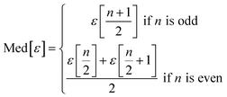
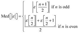
We use seven different statistical metrics to evaluate the fit and predictive ability of a given model. We use the median residual, Med[ε], in eqn (1), the mean absolute residual,  , in eqn (2), median absolute residual, Med[|ε|], in eqn (3) Mean Absolute Percent Error (MAPE) in eqn (4), Akaike Information Criteria (AIC) for normally distributed error in eqn (5), and the percentage of predictions within 5 wt% and 10 wt% of the experimental values.
 | (1) |
 | (2) |
 | (3) |
 | (4) |
 | (5) |
The Med[ε] statistic reveals any bias in the parameter estimation. An unbiased Med[ε] is zero, meaning the same number of residuals are below zero as are above zero. The values for  , Med[|ε|] and MAPE demonstrate how close the model predictions are to the experimental data. AIC is a relative measure of goodness of fit leveraging the likelihood function while avoiding over-fitting the model by penalizing use of an unnecessarily large number of fitted parameters. A low AIC indicates that the error is randomly distributed based on a normal distribution weighed against the number of parameters. The AIC metric is a relative score to compare models. The score is only meaningful if the parameters are the optimal (fitted) parameters for the data used.
3 Component additivity model
A component additivity model is an algebraic expression as in eqn (6) that uses the composition of a biomass feedstock to predict some outcome from HTL. These outcomes typically focus on the biocrude and have included its heating value, elemental composition, and yield YB.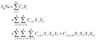 | (6) |
Initial component additivity models for HTL considered just a single time and temperature combination and their predictions were limited to HTL conditions near that single combination. Subsequent component additivity models incorporated the effects of temperature and time, often by using different discrete sets of parameters for different HTL times and temperatures.9–12 A general model for HTL needs to account for the influences of reaction time and temperature, ideally as a continuous function. Herein we use the severity index (SI) (eqn (7)) to combine the effects of time and temperature into a single variable.
 | (7) |
When the reactor heating profile was provided in the publication, we modeled the reactor temperature as a function of time using a Morse-like potential shown in eqn (8). Otherwise, the reaction is treated as isothermal.
 | (8) |
 | (9) |
 | (10) |
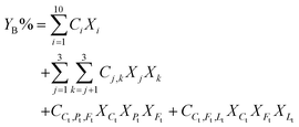
We fit the models using Python version 3.11.7, 64-bit. We used the minimize function from the scipy.optimize version 1.13.0 library with the Nelder–Mead method to minimize the sum of absolute residuals in eqn (2).14 The component additivity model that best fits and predicts the collected data for biocrude yields from HTL of biomass is shown in eqn (11). The C parameters are functions of the severity index and the biomass loading (wt%), per eqn (9). Numerical values for the C parameters for this model at different values of SI and different biomass loadings are provided in Table S1.† There are 15 C parameters and 150 parameters in total. Table 1 gives the parameters evaluated at different values of ln(SI) at 10% loading mass and different loading masses at ln(SI) = 1.64.
 | (11) |
| Parameters | Parameters evaluated at different ln(SI) and fixed 10 (gsolids/gwater)% loading | Parameters evaluated at different loadings (gsolids/gwater) % and fixed ln(SI) = 1.64 which corresponds to 350 °C and 30 min | ||||||||||||
|---|---|---|---|---|---|---|---|---|---|---|---|---|---|---|
| ln(SI) | −10 | −5 | −2.5 | 0 | 2.5 | 5 | 10 | 1.64 | 1.64 | 1.64 | 1.64 | 1.64 | 1.64 | 1.64 |
| Loading mass | 10 | 10 | 10 | 10 | 10 | 10 | 10 | 2.5 | 5 | 10 | 15 | 20 | 25 | 30 |
| C St | 1.82 | 1.81 | 2.17 | 7.18 | 8.34 | 8.35 | 8.33 | 26.7 | 18.9 | 8.28 | 3.24 | 1.21 | 0.444 | 0.162 |
| C Ce | 2.57 | 1.44 | 4.18 | 10.0 | 12.0 | 11.3 | 8.96 | 16.0 | 14.7 | 11.8 | 9.06 | 6.60 | 4.61 | 3.12 |
| C He | 8.20 | 7.99 | 6.85 | 26.8 | 28.5 | 11.2 | 8.24 | 55.1 | 51.9 | 38.5 | 25.0 | 14.7 | 8.07 | 4.25 |
| C Pe | 16.0 | 16.0 | 16.0 | 16.0 | 18.5 | 18.5 | 18.5 | 4.47 × 10⁻⁷ | 0.000185 | 18.5 | 44.9 | 44.9 | 44.9 | 44.9 |
| C Lp | 63.3 | 70.5 | 75.5 | 80.5 | 78.9 | 49.0 | 30.3 | 61.4 | 69.3 | 81.4 | 88.5 | 91.4 | 90.1 | 83.3 |
| C Lg | 0.894 | 0.894 | 0.894 | 2.35 | 14.9 | 0.894 | 0.894 | 0.0692 | 5.46 | 14.7 | 20.6 | 23.7 | 25.1 | 25.7 |
| C Sa | 1.19 × 10⁻⁵ | 2.49 × 10⁻⁵ | 1.57 | 1.57 | 0.930 | 1.19 × 10⁻⁵ | 1.19 × 10⁻⁵ | 0.515 | 0.884 | 1.57 | 2.15 | 2.62 | 2.98 | 3.25 |
| C AA | 1.02 | 1.02 | 1.02 | 1.05 | 1.33 | 3.61 | 0.258 | 0.237 | 0.554 | 1.16 | 1.72 | 2.19 | 2.58 | 2.89 |
| C FA | 36.3 | 49.6 | 55.6 | 60.3 | 15.9 | 15.0 | 17.2 | 0.0160 | 64.3 | 62.6 | 60.9 | 59.3 | 57.6 | 56.0 |
| C Ph | 28.8 | 41.1 | 47.1 | 47.1 | 26.3 | 3.88 | 2.98 | 0.0584 | 29.0 | 36.1 | 36.2 | 36.2 | 36.2 | 36.2 |
| C C t,Pt | −27.1 | −10.1 | 10.2 | 39.8 | 37.8 | −62.9 | −40.4 | 46.7 | 49.3 | 54.4 | 59.3 | −27.9 | −23.7 | −19.9 |
| C C t,Ft | 13.8 | 27.0 | 33.3 | −22.8 | −18.6 | −15.3 | −11.3 | −5.93 | −52.4 | −20.0 | −6.23 | −1.81 | −0.516 | −0.146 |
| C P t,Ft | −92.2 | −92.2 | −92.2 | −92.2 | −92.2 | −92.2 | 91.8 | 86.7 | 90.3 | −92.2 | −86.4 | −79.3 | −72.5 | −65.9 |
| C C t,Pt,Ft | −366 | −137 | 65.7 | 308 | 542 | 727 | 925 | 268 | 344 | 466 | −38.6 | −13.6 | −4.65 | −1.57 |
| C C t,Pt,Lt | 125 | 248 | 225 | 180 | 132 | 90.0 | 36.7 | −155 | −151 | 148 | 131 | 115 | 99.7 | 85.7 |
This model is a simpler version of the more general model in eqn (6). Analysis of that more general model revealed that many interaction terms were statistically insignificant and could be omitted. More specifically, we were able to combine cellulose and the uncategorized carbohydrates into a single biomass pseudo-component. This consolidation reduced the number of individual biomass components to 10 (from 11). We also determined that many interactions involving total lignin were statistically insignificant. Binary interactions are only between Ct, Pt, and Ft.
The values of Ci represent the expected yield of biocrude from HTL of that component alone at the given conditions. For the three carbohydrates, note that Ci decreases as the biomass loading increases. This trend aligns with and is influenced by the data from Gollakota and Savage,15 which showed the biocrude yield decreasing with increasing biomass loading for HTL of polysaccharides. For nearly all of the individual biomass components, the biocrude yield (Ci) first increases and then decreases with increasing reaction severity.
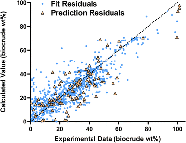
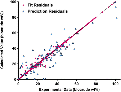
Fig. 1 compares the calculated and experimental biocrude yields for the data set used to fit and predictions for the model parameters. Table 2 summarizes the statistics for each. The model predicts biocrude yields to within 6.3 wt% median absolute error.
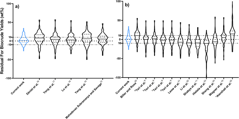
Fig. 2 compares predictions from the new component additivity model with predictions from 17 component additivity models9–12,16–25 in the literature, using the parameters provided in literature. We tested five models capable of predicting biocrude yields from HTL of lignin-containing biomass, shown in Fig. 2a, and 12 models that did not include lignin as part of the composition, shown in Fig. 2b. The models without lignin were tested on the subset of the prediction dataset that contained no lignin-containing biomass. Statistical details are available in Tables S2 and S3† in the ESI.† The new model provides the best predictions, both statistically and visually, compared to the published component additivity models.
In addition to comparing the new model to the published models with the published parameters, we fitted the general forms of these published models to the large datasets to get updated parameter values. Even here, the predictions from the new model were superior to those from the published models.
4 Reaction engineering model
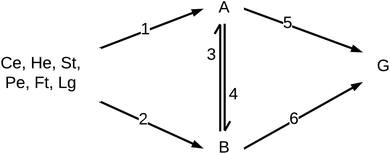
Reaction engineering models are based on chemical reaction networks that describe the conversion of material from one chemical component to another (e.g., from biomass to biocrude). Combining reaction rate equations for each path in the network with the design equation for the type of chemical reactor used in the HTL experiments leads to a set of simultaneous equations that govern the evolution of species concentrations over time. All the biocrude yields in the database used herein were obtained in batch reactors, and we used the appropriate set of differential equations for the modeling. We used mass action rate equations and Arrhenius rate constants. The Arrhenius parameters served as the fitted parameters.A general reaction engineering model for HTL of biomass would include all the biopolymers likely to be in biomass as reactants, allow each to react at its own rate, and account for interactions between biochemical components that influence the yields of product fractions. A general model would also be able to handle smaller biomolecules such as amino acids, saccharides, phenolics, and fatty acids, that are not in polymeric form. The model developed herein meets these criteria. Biomass is treated as a mixture of protein, lipids, lignin, and carbohydrates. The final group is subdivided into cellulose, hemicellulose, and starch, to account for reactivity differences for these polysaccharides. Carbohydrates that are not clearly identified as one of these three in the published work are treated as cellulose for modeling purposes. The reaction network (Fig. 3) allows for binary interactions between carbohydrates, proteins, lipids, and lignin in the biomass as they react to form aqueous-phase (A) and biocrude (B) products. Products in the aqueous phase can react to form gases (G) or molecules that partition into the biocrude phase. Likewise, molecules in the biocrude phase can react to form a water-soluble product or a gaseous product.
Eqn (12) provides the governing differential equations.
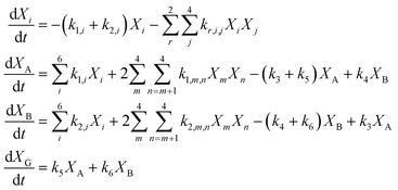 | (12) |
The HTL products are defined operationally as being gases, solids, or material soluble in water or in an organic solvent (biocrude). In many instances, material present in the original, unreacted biomass can be extracted by water or an organic solvent. Accordingly, these systems would contain “biocrude” molecules and “aqueous-phase product” molecules, even before HTL takes place. The initial conditions for the present model accounts for these materials being extractable into those phases at t = 0, before the HTL reaction has begun. We take all lipids and fatty acids to be in the biocrude phase at t = 0. We also take 60 wt% of any phenolics present and 30% of any amino acids initially present in the feedstock to be in the biocrude phase.26 The balance of these smaller biomolecules would reside in the aqueous phase, along with any saccharides initially present in the biomass feedstock. We take 46 wt% of the protein, 3 wt% of the hemicellulose, and 11 wt% of the starch to be in the aqueous phase at t = 0.27 The rest of the biopolymers in the biomass feedstock are taken to reside in the solid phase when HTL begins. Through the use of the reaction network for the biopolymers and product fractions and these initial conditions for any smaller biomolecules, we have developed a general model that can be applied to a wide range of biomass feedstocks. We assume the interactions of the other biopolymers with the polysaccharides (Ps), cellulose, hemicellulose and starch, is identical. Fitting the model to the large dataset gives the parameter values in Table 3. The model has 56 parameters.
| Parameter label | ln[A] (ln[min−1]) | E a (kJ mol−1) | k @350 °C (min−1) | Parameter label | ln[A] (ln[min−1]) | E a (kJ mol−1) | k @350 °C (min−1) |
|---|---|---|---|---|---|---|---|
| k 1,Pe | −0.107 | 0.00860 | 0.897 | k 1,Pe,Ft | 40.6 | 203 | 4.26 |
| k 1,Ft | 10.2 | 33.5 | 40.7 | k 1,Pe,Ps | 10.9 | 105 | 9.04 × 10⁻⁵ |
| k 1,Ce | 7.55 | 47.9 | 0.184 | k 1,Pe,Lg | 20.6 | 85.5 | 62.7 |
| k 1,He | 13.8 | 88.1 | 0.0387 | k 1,Ft,Ps | 7.88 | 25.2 | 20.2 |
| k 1,St | 7.42 | 40.5 | 0.668 | k 1,Ft,Lg | 4.73 | 1.33 | 87.6 |
| k 1,Lg | −2.82 | 4.35 | 0.0257 | k 1,Ps,Lg | 45.3 | 248 | 0.0758 |
| k 2,Pe | 0.370 | 5.18 | 0.533 | k 2,Pe,Ft | 15.4 | 54.5 | 126 |
| k 2,Ft | 1.73 | 3.39 | 2.93 | k 2,Pe,Ps | 9.62 | 49.7 | 1.02 |
| k 2,Ce | 10.1 | 69.9 | 0.0353 | k 2,Pe,Lg | 4.47 | 17.9 | 2.74 |
| k 2,He | 14.3 | 86.8 | 0.0887 | k 2,Ft,Ps | 16.0 | 57.4 | 133 |
| k 2,St | 9.18 | 58.7 | 0.116 | k 2,Ft,Lg | 19.1 | 36.7 | 1.66 × 10⁵ |
| k 2,Lg | −2.05 | 13.9 | 0.00872 | k 2,Ps,Lg | 25.7 | 227 | 1.35 × 10⁻⁸ |
| k 3 | 6.30 | 214 | 6.07 × 10⁻¹⁶ | k 5 | −2.86 | 10.9 | 0.00696 |
| k 4 | 2.11 | 48.9 | 0.00066 | k 6 | 14.3 | 107 | 0.00181 |
We fit all the models in Python version 3.11.7, 64-bit using solve_ivp from scipy.integrate version 1.13.0 with the Radau stiff solver to calculate the numerical solution for the system of ODEs. We used the minimize function from the scipy.optimize library with the Nelder–Mead method to minimize the sum of absolute residuals in eqn (2).14
Fig. 4 compares the calculated and experimental biocrude yields for the data set used to fit and predictions for the model parameters. Table 4 summarizes the statistics for each. The model is able to correlate and predict biocrude yields with an median absolute residual of about 5.5 wt%.
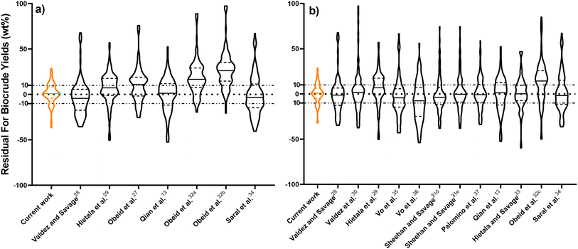
Fig. 5 compares predictions from the new reaction engineering model to predictions from 15 reaction engineering models13,27–37 in the literature. Fig. 5a displays violin plots of the distribution of residuals for the new model, three models that explicitly include lignin in biomass, and four models that do not require biomass composition. The new model gives better predictions. Fig. 5b displays violin plots of the distribution of residuals for the new reaction engineering model and eight models that do not include lignin as part of the biomass. We include data only from HTL of the lignin-void biomass in the testing dataset in Fig. 5b. All the statistical data is provided in the ESI in Tables S2 and S3.†
We also fit the parameters for the reaction networks from Valdez et al.,30 Sheehan and Savage,31 Obeid et al.,32 and Hietala and Savage33 to the new, larger dataset. The statistics for biocrude fit and predictions are available in Tables S6 and S7.† The results show the new reaction engineering model is superior to the other networks using the same dataset to parameterize all the models.
5 Machine learning model
Machine learning models explain and predict outputs by identifying the connections and patterns between inputs and outputs. These models require user input parameters such as the number of estimators and minimization criteria. To determine the optimal parameters for predictions, we separate the fitting dataset, 90% of the total dataset, into 80% training and 20% testing data subsets. While varying the user input parameters, we optimized the predictions for the 20% testing data subset. We then fit the model to the full 90% fitting dataset and used the optimal parameters to predict the 10% prediction dataset.We tested supervised, continuous input and output machine learning models. The model algorithms are from the sklearn version 1.4.0 library in Python version 3.11.7, 64-bit.38
Of all the machine learning models, the decision tree algorithm provided the highest performance in fitting and predicting of the data. The model is set to a maximum depth of 14, three random states, the minimization criterion set to absolute error, and the rest of the options as default choices. The model results in a 924-leaf tree network. We provide the code on GitHub (https://github.com/pguirguis/Model_Comparison) to print the tree and use it for predictions. The Gaussian Process Algorithm has the optimal statistics (see the ESI†), but its Gaussian structure does not align with the relationship between the HTL conditions and biocrude yields, resulting in a distinct inability to predict the data accurately. Additionally, the random forest algorithm shows a good fit and the outstanding prediction with 7241 leaves. However, this model is not chosen because its AIC is four times that of the decision tree algorithm. Tables S8–S11† provide statistics for all models that we considered.
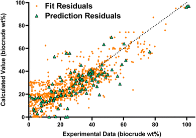
Fig. 6 compares the calculated and experimental biocrude yields for the data set used to fit and predictions for the model parameters. Table 5 summarizes the statistics for each. The model predicted biocrude yields to within 4.6 wt% median absolute residual.
6 Comparing the new models
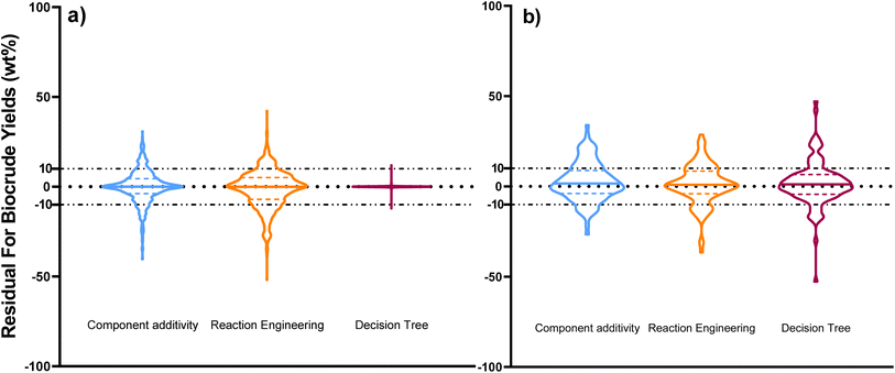
Fig. 7 shows the distribution of the residuals for all three models. Fig. 7a is the distribution for fitting each model to the literature dataset and Fig. 7b is the distribution for predictions. The decision tree model fits the data the best. It also has the largest number of parameters, with 924 leaves. The model uses a set of “decisions” to reach its predictions, and 868 out of the 924 leaves contain a single data point. The component additivity model, with 150 parameters, has lower error than the reaction engineering model, which has 56 parameters. The component additivity model uses additional parameters to correlate and predict the effects of biomass loading (wt%). For predictions, the decision tree model had the smallest median absolute error of 4.6 wt%, but it also gives the widest distribution of residuals. The component additivity model has the smallest distribution of residuals and its median absolute error was 6.33 wt%. The reaction engineering model performed similarly and has a median absolute residual of 5.53 wt%.7 Predictions for new biomass feedstocks
In this section, we use the new models to estimate the highest biocrude yields available from HTL of different biomass feedstocks, along with the corresponding HTL conditions. The feedstocks and their compositions are listed in Table 6. Three feedstocks have a high carbohydrate content. One is high in cellulose (hemp fiber), one is high in starch (macaroni noodles), and one is high in other carbohydrates (watermelon rinds). We selected one feedstock with high lipid content, which also has the highest protein content (mechanically deboned chicken meat), and one with high lignin content (apple pomace). In nature, biomass with high hemicellulose or lignin content typically also contains a significant amount of cellulose. The apricot kernel press cake contains all four components in relatively balanced proportions. Cheese sauce contains nearly equal amounts of starch and protein, along with lipids. Finally, we considered the mixture of cheese sauce and macaroni, as described in Wang et al.44| Ref. | Feedstock | C t | Un | Ce | He | St | P t | F t | L t | Ash |
|---|---|---|---|---|---|---|---|---|---|---|
| Jawaid and Abdul Khalil39 | Hemp fiber | 92.3 | 0 | 74.4 | 17.9 | 0 | 0 | 1.30 | 3.70 | N/A |
| Arivuchudar40 | Watermelon rinds | 62.8 | 62.8 | 0 | 0 | 0 | 12.5 | 2.74 | 0 | 14.7 |
| Selmane et al.41 | Mechanically deboned chicken meat | 0 | 0 | 0 | 0 | 0 | 52.7 | 42.5 | 0 | N/A |
| Vendruscolo et al.42 | Apple pomace | 59.8 | 59.8 | 0 | 0 | 0 | 5.90 | 0 | 38.2 | 3.50 |
| Sharma et al.43 | Apricot kernel press cake | 27.5 | 27.5 | 0 | 0 | 0 | 34.3 | 9.70 | 10.8 | N/A |
| Wang et al.44 | Cooked macaroni noodles | 83.9 | 0 | 0 | 0 | 83.9 | 14.0 | 1.35 | 0 | 0.800 |
| Cheese sauce | 42.9 | 0 | 0 | 0 | 42.9 | 41.5 | 12.6 | 0 | 3.03 | |
| Macaroni and cheese | 70.9 | 0 | 0 | 0 | 70.9 | 13.5 | 14.1 | 0 | 1.51 |
Table 7 presents the conditions for HTL predicted by each model to give the highest possible biocrude yield.
| Ref. | Feedstock | Component additivity model | Reaction engineering model | Decision tree model | ||||||||||
|---|---|---|---|---|---|---|---|---|---|---|---|---|---|---|
| Biocrude (wt%) | Solids (g g−1 %) | ln(SI) | Biocrude (wt%) | Time (min) | Temp. (°C) | *b (min−1) | ln(SI) | Biocrude (wt%) | Solids (g g−1 %) | Time (min) | Temp. (°C) | ln(SI) | ||
| a *b is the constant for the heating profile in eqn (8). N/A means the model did not move that value from its initial state, Iso means isothermal. | ||||||||||||||
| Jawaid and Abdul Khalil39 | Hemp fiber | 28.2 | 1.87 | 1.23 | 31.5 | 0.770 | 556 | Iso | 1.96 | 22.1 | N/A | N/A | 480 | N/A |
| Arivuchudar40 | Watermelon rinds | 22.5 | 10.7 | 1.76 | 31.8 | 0.656 | 560 | Iso | 1.86 | 17.0 | 29.0 | 15.5 | 328 | 1.02 |
| Selmane et al.41 | Mechanically deboned chicken meat | 63.9 | 12.5 | 6.05 | 54.1 | 2.84 | 388 | Iso | 0.212 | 66.0 | 13.4 | 1.03 | 575 | 2.52 |
| Vendruscolo et al.42 | Apple pomace | 22.8 | 17.7 | 1.84 | 20.3 | 152 | 328 | 1.99 | 2.67 | 23.1 | N/A | N/A | 475 | N/A |
| Sharma et al.43 | Apricot kernel press cake | 36.7 | 18.4 | 1.60 | 47.4 | 1.37 | 479 | Iso | 1.30 | 66.0 | 13.4 | 1.03 | 575 | 2.52 |
| Wang et al.44 | Cooked macaroni noodles | 39.4 | N/A | 1.71 | 36.5 | 0.322 | 591 | Iso | 1.55 | 32.0 | N/A | 2.83 | 313 | −1.73 |
| Cheese sauce | 49.1 | 0.734 | 1.75 | 48.7 | 1.39 | 467 | Iso | 1.09 | 66.0 | 13.4 | 1.03 | 575 | 2.52 | |
| Macaroni and cheese | 51.1 | 0.185 | 1.69 | 41.9 | 0.475 | 542 | Iso | 1.26 | 66.0 | 13.4 | 1.03 | 575 | 2.52 | |
Since the machine learning model is made of discrete choices, we use a grid of 1000 steps for time between 0–3 h, loading mass between 0–40 (g solids/g water)%, and temperature between 0–650 °C to find the maximum biocrude yield. The decision tree model uses discrete “decisions” or “leaves” to fit the data, which aligns the predictions closely with the correlating data. The large number of “N/A” entries in Table 7 for the decision tree model however, indicates the model has difficulty with feedstocks that do not closely match those used to determine the parameters. Additionally, predictions for four out of the eight feedstocks give the same yield and HTL conditions despite the feedstocks having very different compositions. This is a disadvantage of using a discrete model such as the decision tree. When examining predictions for a larger dataset of 39 new biomass feedstocks, we find only 11 unique optimal conditions for the decision tree machine learning model.
The three models agree that HTL of the biomasses with large fractions of carbohydrates have a lower maximum biocrude yield than the other feedstocks. Additionally, HTL of mechanically deboned chicken meat, high in fat and proteins, gives the highest biocrude yield for each model. Finally, all the models predict a higher biocrude yield for HTL of the macaroni and cheese together rather than separately. The predicted increase in biocrude yield is 8.75 wt%, 1.56 wt%, and 23.25 wt% for component additivity model, reaction engineering model, and decision tree model, respectively.
The models show large disagreement for HTL conditions for a few feedstocks. For mechanically deboned chicken meat and cheese sauce, the reaction engineering model predicts milder conditions than does the component additivity model. The models also disagree as to the reaction severity needed to liquefy the cooked macaroni noodles, cheese sauce, and macaroni and cheese. The decision tree model has the highest severity, the component additivity model has a medium severity, and the reaction engineering model gives the mildest conditions.
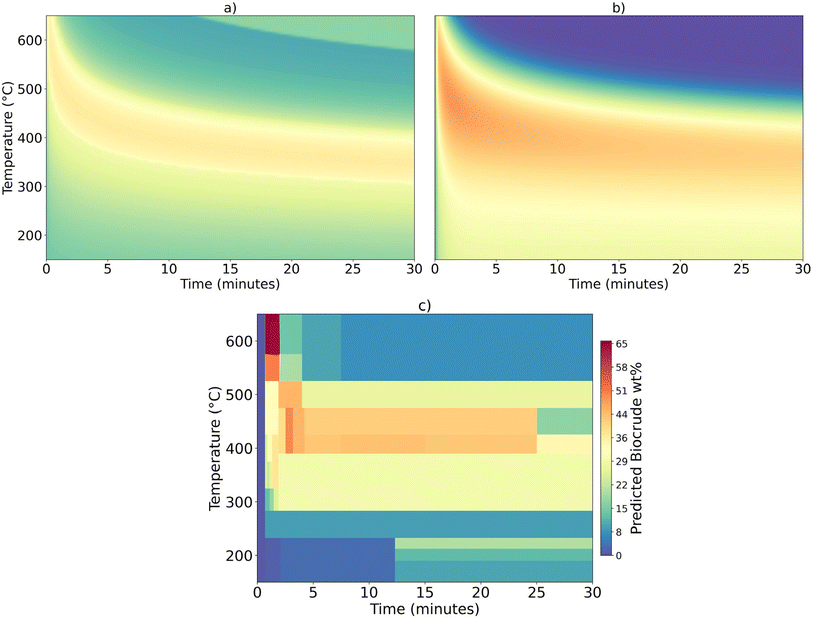
The apricot kernel press cake is the only new feedstock considered here that contains at least 10% each of carbohydrates, proteins, lipids, and lignin. Containing all these components in appreciable amounts makes this material an interesting biomass feedstock for testing the models. The three models disagree on the severity of the HTL conditions and the highest biocrude yield that can be obtained. Fig. 8 examines HTL of this feedstock in greater detail. The figure shows the biocrude yields calculated from each model over a wide range of HTL temperatures and times. The colors correspond to the biocrude yields. Fig. 8a shows the component additivity model predicts biocrude yields up to about 35 wt% follow a narrow band on the plot. Fig. 8b shows the reaction engineering model predicts biocrude yields of about 50 wt% at short times over a range of supercritical temperatures. Fig. 8c shows discrete “decision” boxes and there are no smooth transitions between the boxes.
8 Closing perspective
This work provides new models for predicting yields of biocrude from HTL of biomass. These models predicted literature data better than did previous models. The highest median absolute residual for predicting the biocrude yields was 6.3 wt%. The decision tree model fit and predicted the dataset significantly better than the new component additivity and reaction engineering models. The component additivity model is statistically better at fitting the dataset than the reaction engineering model and the reaction engineering model is better at predicting the dataset than the component additivity model. When seeking the optimal HTL conditions for new feedstocks, the discrete “leaves” from the decision tree model limits the model predictions.The models are general in that they can be applied to nearly any biomass feedstock and over a very wide range of potential HTL reaction conditions. As such, the models can be used to guide experimental work. They can also be employed in technoeconomic analyses and life cycle assessments to investigate the influence of biomass composition and HTL processing conditions on the profitability and environmental impacts of HTL conversion.
The present modeling work accepted all literature data as being of equal value. We believe even better models could be developed if there were a carefully curated set of experimental data for HTL. Ideally, the same biomass feedstocks and same sets of reaction conditions would be examined in multiple labs and the resulting data then combined and assessed. Such a harmonized data set, which would include experimental uncertainties, would be a tremendous asset in improving the general models for HTL of biomass.
The three different approaches for modeling used herein have comparative advantages and disadvantages. Component additivity models are conceptually simple and provide a connection to the physical system. They can be expanded as needed to account for statistically meaningful interactions between components. Decision tree models can do a great job of fitting data, but the predictive ability is not as good as the correlating ability (at least in the present study). Also, the decision tree has no connection to the physical situation and it is a discrete model whereas process variables are continuous. Reaction engineering models can provide predictions for all components in the reacting system – not just biocrude. That is, the model can predict (or correlate) the yields of aqueous-phase products and gaseous products as well. Moreover, a reaction engineering model can be made even more “molecular” by adopting reaction pathways that are more closely connected to the overall chemical conversions taking place (e.g., protein decomposing to peptides that decompose to amino acids that decomposes further by deamination or decarboxylation).
Each model has limitations. Using the severity index in the component additivity model ignores the individual effects of time and temperature. As a result, the conditions obtained when optimizing feedstocks include a set of temperature and time for the optimal severity index. The reaction engineering model is the only model that does not include any dependence of HTL outcomes on the wt% loading in the reactor, though this is known to have an effect for some biomass components. The decision tree model predicts biocrude yields based on given feedstock composition and HTL conditions. Its accuracy depends on the similarity between the input data and the training set. When inputs closely match the training data, predictions are reliable. However, if the training set lacks similar feedstock compositions and HTL conditions, the model may produce inaccurate predictions. With a large training dataset and numerous input parameters, identifying the specific feedstock compositions and HTL conditions needed to prevent inaccurate predictions becomes challenging. This limitation is evident when optimizing HTL conditions for the feedstocks tested in this study.
Data availability
The three models and the data associated with them are available on GitHub (https://github.com/pguirguis/Model_Comparison).Author contributions
Peter M. Guirguis: conceptualization, data curation, formal analysis, validation, visualization, writing – original draft, writing – review & editing, and Phillip E. Savage: conceptualization, funding acquisition, methodology, project administration, supervision, writing – review & editing.Conflicts of interest
There are no conflicts to declare.Acknowledgements
This work was supported with funds from the Walter L. Robb Family Chair in Chemical Engineering at Penn State.Notes and references
- M. Shahabuddin, N. Kazantzis, A. R. Teixeira and M. T. Timko, Energy Convers. Manage.:X, 2024, 24, 100756 Search PubMed.
- Y. Jiang, S. B. Jones, Y. Zhu, L. Snowden-Swan, A. J. Schmidt, J. M. Billing and D. Anderson, Algal Res., 2019, 39, 101450 CrossRef.
- P. H. Chen and J. C. Quinn, Appl. Energy, 2021, 289, 116613 CrossRef CAS.
- M. Pearce, M. Shemfe and C. Sansom, Appl. Energy, 2016, 166, 19–26 CrossRef.
- L. Ou, R. Thilakaratne, R. C. Brown and M. M. Wright, Biomass Bioenergy, 2015, 72, 45–54 CrossRef CAS.
- P. Ranganathan and S. Savithri, Bioresour. Technol., 2019, 284, 256–265 CrossRef CAS PubMed.
- Y. Zhu, M. J. Biddy, S. B. Jones, D. C. Elliott and A. J. Schmidt, Appl. Energy, 2014, 129, 384–394 CrossRef CAS.
- P. M. Guirguis, M. S. Seshasayee, B. Motavaf and P. E. Savage, RSC Sustainability, 2024, 2, 736–756 RSC.
- G. Teri, L. Luo and P. E. Savage, Energy Fuels, 2014, 28, 7501–7509 CrossRef CAS.
- J. Wagner, R. Bransgrove, T. A. Beacham, M. J. Allen, K. Meixner, B. Drosg, V. P. Ting and C. J. Chuck, Bioresour. Technol., 2016, 207, 166–174 CrossRef CAS PubMed.
- R. Shakya, S. Adhikari, R. Mahadevan, S. R. Shanmugam, H. Nam, E. B. Hassan and T. A. Dempster, Bioresour. Technol., 2017, 243, 1112–1120 CrossRef CAS PubMed.
- S. Mahadevan Subramanya and P. E. Savage, ACS Sustain. Chem. Eng., 2021, 9, 13874–13882 CrossRef CAS.
- L. Qian, S. Wang and P. E. Savage, Appl. Energy, 2020, 260, 114312 CrossRef CAS.
- P. Virtanen, R. Gommers, T. E. Oliphant, M. Haberland, T. Reddy, D. Cournapeau, E. Burovski, P. Peterson, W. Weckesser, J. Bright, S. J. van der Walt, M. Brett, J. Wilson, K. J. Millman, N. Mayorov, A. R. J. Nelson, E. Jones, R. Kern, E. Larson, C. J. Carey, Ä. Polat, Y. Feng, E. W. Moore, J. VanderPlas, D. Laxalde, J. Perktold, R. Cimrman, I. Henriksen, E. A. Quintero, C. R. Harris, A. M. Archibald, A. H. Ribeiro, F. Pedregosa, P. van Mulbregt, A. Vijaykumar, A. P. Bardelli, A. Rothberg, A. Hilboll, A. Kloeckner, A. Scopatz, A. Lee, A. Rokem, C. N. Woods, C. Fulton, C. Masson, C. Häggström, C. Fitzgerald, D. A. Nicholson, D. R. Hagen, D. V. Pasechnik, E. Olivetti, E. Martin, E. Wieser, F. Silva, F. Lenders, F. Wilhelm, G. Young, G. A. Price, G.-L. Ingold, G. E. Allen, G. R. Lee, H. Audren, I. Probst, J. P. Dietrich, J. Silterra, J. T. Webber, J. Slavič, J. Nothman, J. Buchner, J. Kulick, J. L. Schönberger, J. V. de Miranda Cardoso, J. Reimer, J. Harrington, J. L. C. Rodríguez, J. Nunez-Iglesias, J. Kuczynski, K. Tritz, M. Thoma, M. Newville, M. Kümmerer, M. Bolingbroke, M. Tartre, M. Pak, N. J. Smith, N. Nowaczyk, N. Shebanov, O. Pavlyk, P. A. Brodtkorb, P. Lee, R. T. McGibbon, R. Feldbauer, S. Lewis, S. Tygier, S. Sievert, S. Vigna, S. Peterson, S. More, T. Pudlik, T. Oshima, T. J. Pingel, T. P. Robitaille, T. Spura, T. R. Jones, T. Cera, T. Leslie, T. Zito, T. Krauss, U. Upadhyay, Y. O. Halchenko and Y. Vázquez-Baeza, Nat. Methods, 2020, 17, 261–272 CrossRef CAS PubMed.
- A. Gollakota and P. E. Savage, Energy Fuels, 2019, 33, 11328–11338 CrossRef CAS.
- M. Déniel, G. Haarlemmer, A. Roubaud, E. Weiss-Hortala and J. Fages, Waste Biomass Valorization, 2017, 8, 2087–2107 CrossRef.
- J. Yang, Q. S. He, H. Niu, K. Corscadden and T. Astatkie, Appl. Energy, 2018, 228, 1618–1628 CrossRef CAS.
- J. Lu, Z. Liu, Y. Zhang and P. E. Savage, ACS Sustain. Chem. Eng., 2018, 6, 14501–14509 CrossRef CAS.
- J. Yang, Q. S. He, K. Corscadden, H. Niu, J. Lin and T. Astatkie, Appl. Energy, 2019, 233–234, 906–915 CrossRef CAS.
- P. Biller and A. B. Ross, Bioresour. Technol., 2011, 102, 215–225 CrossRef CAS PubMed.
- S. Leow, J. R. Witter, D. R. Vardon, B. K. Sharma, J. S. Guest and T. J. Strathmann, Green Chem., 2015, 17, 3584–3599 RSC.
- Y. Li, S. Leow, A. C. Fedders, B. K. Sharma, J. S. Guest and T. J. Strathmann, Green Chem., 2017, 19, 1163–1174 RSC.
- D. C. Hietala, C. K. Koss, A. Narwani, A. R. Lashaway, C. M. Godwin, B. J. Cardinale and P. E. Savage, Algal Res., 2017, 26, 203–214 CrossRef.
- L. Sheng, X. Wang and X. Yang, Bioresour. Technol., 2018, 247, 14–20 CrossRef CAS PubMed.
- A. Aierzhati, M. J. Stablein, N. E. Wu, C.-T. Kuo, B. Si, X. Kang and Y. Zhang, Bioresour. Technol., 2019, 284, 139–147 CrossRef CAS PubMed.
- R. Obeid, D. M. Lewis, N. Smith, T. Hall and P. van Eyk, Chem. Eng. J., 2020, 389, 124397 CrossRef CAS.
- R. Obeid, D. M. Lewis, N. Smith, T. Hall and P. van Eyk, Energy Fuels, 2020, 34, 419–429 CrossRef CAS.
- P. J. Valdez and P. E. Savage, Algal Res., 2013, 2, 416–425 CrossRef.
- D. C. Hietala, J. L. Faeth and P. E. Savage, Bioresour. Technol., 2016, 214, 102–111 CrossRef CAS PubMed.
- P. J. Valdez, V. J. Tocco and P. E. Savage, Bioresour. Technol., 2014, 163, 123–127 CrossRef CAS PubMed.
- J. D. Sheehan and P. E. Savage, Bioresour. Technol., 2017, 239, 144–150 CrossRef CAS PubMed.
- R. Obeid, N. Smith, D. M. Lewis, T. Hall and P. van Eyk, Chem. Eng. J., 2022, 428, 131228 CrossRef CAS.
- D. C. Hietala and P. E. Savage, Chem. Eng. J., 2021, 407, 127007 CrossRef CAS.
- J. S. Saral, D. G. C. V. Reddy and P. Ranganathan, Biomass Convers. Biorefin., 2022, 1, 1–9 Search PubMed.
- T. K. Vo, O. K. Lee, E. Y. Lee, C. H. Kim, J.-W. Seo, J. Kim and S.-S. Kim, Chem. Eng. J., 2016, 306, 763–771 CrossRef CAS.
- T. K. Vo, S.-S. Kim, H. V. Ly, E. Y. Lee, C.-G. Lee and J. Kim, Bioresour. Technol., 2017, 241, 610–619 CrossRef CAS PubMed.
- A. Palomino, L. C. Montenegro-Ruíz and R. D. Godoy-Silva, Algal Res., 2019, 44, 101669 CrossRef.
- F. Pedregosa, G. Varoquaux, A. Gramfort, V. Michel, B. Thirion, O. Grisel, M. Blondel, P. Prettenhofer, R. Weiss, V. Dubourg, J. Vanderplas, A. Passos, D. Cournapeau, M. Brucher, M. Perrot and E. Duchesnay, J. Mach. Learn. Res., 2011, 12, 2825–2830 Search PubMed.
- M. Jawaid and H. Abdul Khalil, Carbohydr. Polym., 2011, 86, 1–18 CrossRef CAS.
- R. Arivuchudar, Biosci., Biotechnol. Res. Asia, 2023, 20, 263–269 Search PubMed.
- D. Selmane, V. Christophe and D. Gholamreza, Meat Sci., 2008, 79, 640–647 CrossRef CAS PubMed.
- F. Vendruscolo, P. M. Albuquerque, F. Streit, E. Esposito and J. L. Ninow, Crit. Rev. Biotechnol., 2008, 28, 1–12 CrossRef CAS PubMed.
- P. C. Sharma, B. M. K. S. Tilakratne and A. Gupta, J. Food Sci. Technol., 2010, 47, 682–685 CrossRef CAS PubMed.
- Y. Wang, T. D. Wig, J. Tang and L. M. Hallberg, J. Food Eng., 2003, 57, 257–268 CrossRef.
Footnote |
| † Electronic supplementary information (ESI) available. See DOI: https://doi.org/10.1039/d4su00737a |
| This journal is © The Royal Society of Chemistry 2025 |

