Multiscale modelling of nuclear magnetisation dynamics: spin relaxation, polarisation transfer and chemical exchange in ¹²⁹Xe@cryptophane(aq) structures

Abstract

Computational nuclear magnetic resonance (NMR) spectroscopy of supramolecular Xe@cryptophane(aq) complexes requires a multiscale approach due to the interplay of molecular dynamics, spin relaxation, chemical exchange, and solvent effects. The flexible cryptophane cage consists of approximately 150 atoms, including 50 protons, and the encapsulated xenon atom undergoes significant dynamics. Furthermore, the biosensing applications of this structure occur in aqueous, non-deuterated solvents. Consequently, fluctuations in internuclear dipole–dipole (DD) couplings lead to spin relaxation and polarisation transfer between nuclei, with Xe exchange between the solvent and the cage playing a pivotal role. Here, we introduce a novel molecular dynamics (MD)-based approach to simulate DD-driven magnetisation dynamics, incorporating intermolecular relaxation and cross-relaxation effects that are often overlooked in traditional MD–DD modelling. We compute the ¹²⁹Xe and ¹H relaxation times for Xe(aq) and two water-soluble Xe@cryptophane(aq) systems and examine the spin polarisation-induced nuclear Overhauser effect (SPINOE) between hyperpolarised xenon and the surrounding protons, obtaining results in good agreement with the available experimental data. Using a two-site exchange model and first-principles computed Xe chemical shifts, we assess the impact of xenon exchange on observable relaxation and polarisation transfer and simulate the ¹²⁹Xe NMR spectrum, accounting for both chemical exchange and DD relaxation. This work bridges the gap between fully quantum-mechanical spin dynamics simulations and traditional MD–DD approaches and presents the first comprehensive SPINOE modelling and relaxation analysis in xenon biosensor systems.

---

1 Introduction

1.1 Background

1.1.1 Magnetisation dynamics in molecular systems. A nuclear spin ensemble displaced from thermal equilibrium undergoes a combination of coherent time evolution and incoherent relaxation back towards the equilibrium. The resulting, observable NMR signal is the free induction decay (FID) of the macroscopic nuclear magnetisation M(t) = [M_x(t), M_y(t), M_z(t)]^T, where the coherent and incoherent effects are responsible for the oscillation and decay of the signal, respectively. In high-field liquid-state NMR, and in the absence of externally applied radiofrequency fields (i.e., during free evolution), the oscillation frequencies are determined by isotropic spin interactions, whereas molecular dynamics and the resulting incoherent fluctuations of spin interactions contribute to relaxation.¹ The incoherent mechanisms can lead to cross-relaxation, i.e., magnetisation transfer between spins. A famous example is the nuclear Overhauser effect (NOE)² caused by the direct dipole–dipole (DD) coupling. In the presence of hyperpolarised (hp) spins, the NOE is particularly strong and is called spin polarisation-induced NOE (SPINOE).^3–6

In addition to single-molecule dynamics, particularly rotation with respect to the direction of the external magnetic field, the time evolution of M(t) is affected by chemical exchange, which typically occurs on a much slower time scale than the molecular tumbling. Chemical exchange can lead to signal decay, coalescence of spectral peaks and magnetisation transfer between the exchanging sites.¹ In many cases, a satisfactory model for the dynamics of M(t) requires a combination of coherent evolution, spin relaxation and chemical exchange.

A particularly challenging task is the modelling of relaxation. For approximately rigid molecules in isotropic solvents, it is reasonable to assume that isotropic rotational diffusion of a rigid rotor provides a relevant motional model. This approximation can be applied in the framework of NMR relaxation theory to estimate the auto- and cross-relaxation rates of the spins, which can then be used in spin dynamics simulations. However, this model can be too simple for describing conformationally flexible molecules. In addition, it cannot explicitly describe intermolecular relaxation. These features can become important in relatively large and flexible molecules with tens of spins, in solvents of high proton spin density (such as water) and/or when the system includes non-covalently bonded chemical units or atoms. Due to the complexity of such systems, a fully quantum-mechanical treatment of spin dynamics is usually not feasible.

When the DD mechanism dominates relaxation, a usual situation for liquid-phase spin-1/2 systems in the absence of unpaired electrons, relaxation rates can be computed from molecular dynamics (MD) simulation trajectories.^7–15 MD simulations account for all types of motion in the system, and allow straightforward computation of the intermolecular contributions to relaxation.^8,9,14,16,17 As opposed to analytical motional models, no distinction between different motional modes, such as rotation and translation, needs to be made. MD simulations are typically more accurate in describing the internuclear dynamics and, therefore, the DD relaxation rates, than the rigid-rotor model. However, it is a common practice in DD-relaxation modelling with MD simulations (termed MD–DD modelling from now on) to neglect cross-relaxation and, thereby, the resulting polarisation transfer between chemically non-equivalent spins. Hence, although the traditional MD–DD modelling provides a better dynamical description than the rigid-rotor model, the inherently coupled time evolution of spins is not routinely taken into account.

From the modelling point of view, the presence of chemical exchange introduces further difficulties. If it plays an important role in the studied system, the coherent and incoherent mechanisms have to be computed for each exchanging site n. The exchange rates between the sites, within a suitable exchange model, can then be used to simulate the combined time evolution of all the {M⁽ⁿ⁾(t)}. The total size of the combined system is a sum over the sizes of the individual systems, which increases the computational demands.

1.1.2 Xe NMR. Xenon atoms can noncovalently bind to various microscopic pockets and cavities in molecules and materials. Within such environments, interaction takes place between the sensitive electron cloud of the guest and the host, reported by the NMR chemical shift (CS) of the xenon nucleus.^18–21 In the 1990s, Xe was shown to form supramolecular host–guest complexes with organic cage molecules, particularly with cryptophanes (Cr).^22–24 Inside such hosts, the xenon CS can span a range of hundreds of ppm. Among the NMR-active isotopes of xenon, the spin-1/2 ¹²⁹Xe isotope is notable for its relatively high natural abundance of 26% and the absence of rapid quadrupolar relaxation, as compared to the spin-3/2 ¹³¹Xe isotope.

In addition to the favourable chemical and NMR properties of ¹²⁹Xe, the spin-exchange optical pumping (SEOP) method^25,26 can be used to easily hyperpolarise a sample of xenon gas. This process involves transferring the electron spin polarisation of alkali–metal atoms (typically rubidium) to the polarisation of xenon nuclei. SEOP can enhance the Xe NMR signal by a factor of ε = 10⁴ as compared to thermal polarisation at room temperature. Consequently, hp ¹²⁹Xe NMR has found use in the study of porous materials and in medical imaging.^20,27,28

1.1.3 Xe NMR biosensors. Because xenon is a noble gas and, hence, chemically inert, it cannot be used as such to target specific molecules. To overcome this issue, it was demonstrated by the Pines lab in 2001²⁹ that ¹²⁹Xe could be used for molecule-selective chemical sensing after encapsulating it in a functionalised cryptophane cage. Such guest–host complexes are nowadays called xenon biosensors (XBSs).^30–36 The functional unit is a chemical moiety attached onto the cage, designed to bind with a specific target molecule. The binding changes the chemistry of the XBS, the effect is mediated to the sensitive electron cloud of the xenon guest and, finally, the event is reported by the Xe CS.

A direct NMR measurement of Xe is not typically feasible due to the low population of the host-bound site prevailing in typical biosensing situations. Because the binding to the host cage is weak, chemical exchange occurs between the bound and free xenon sites, with ‘free’ here referring to the hp Xe in the bulk solvent. The exchange process is illustrated in Fig. 1 and described by the rate equation

The exchange-rate constants k_± describe the association and dissociation of the Xe@Cage complex, and are related to the exchange rates ν_± and the concentrations as

ν₊ = k₊[Xe][Cage]

ν₋ = k₋[Xe@Cage].

The equilibrium exchange rate is defined as

ν_ex ≡ ν^eq₊ + ν^eq₋. (2)

For most cages, including the Cr structures, ν_ex is of the order of 10²–10³ s⁻¹.^37–47 Because the Xe CS is a sensitive probe of the chemical environment – resulting in a significant change in the NMR frequency ω between the bound and free sites – ν_ex is located in the slow exchange regime, such that . Here, Δω is the difference in the resonance frequencies of the exchanging sites. The binding equilibrium is also characterised by the association constant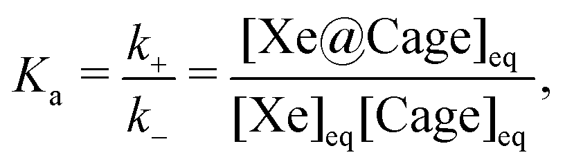with value in the order of 10³–10⁴ M⁻¹.^22,38–52 These characteristics allow the use of the chemical exchange saturation transfer (CEST)⁵³ method, which can enhance the Xe NMR signal by a factor of the order of 10³.

Fig. 1 Chemical exchange of xenon with a cryptophane cage. The 3AC and 6AC cryptophane-A derivatives studied in the present work are composed of two connected cyclotribenzylene (CTB) bowls. The chemical groups attached to the six binding sites of the cages, Rⁱ in the figure, are indicated.

The use of XBSs in low-concentration chemical sensing is founded in the combination of the SEOP and CEST methods in the so-called hyper-CEST experiment.^54–57 There, hp Xe gas is allowed to undergo chemical exchange [eqn (1)] between the solvent and the host cages, with frequency-swept, continuous irradiation applied over the CS range of Xe. Irradiation coinciding with the resonance frequency of the host-bound Xe renders equal the populations of the nuclear spin states, and destroys the longitudinal magnetisation of the bound site at that frequency. As a result of the exchange back to the majority (solution) site, the intensity of the solution-state Xe signal decreases by an amount that depends on the irradiation frequency. When the bulk signal intensity is plotted as a function of the irradiation frequency, in the so-called z-spectrum, the resonance frequencies of the less populated sites are revealed. Hyper-CEST can increase the signal intensity altogether by a factor of 10⁷, which significantly reduces the minimum concentration of the Xe@Cage complexes that can be detected. This was demonstrated in ref. 58 where picomolar detection of cryptophane-based complexes was possible.

1.2 Relaxation

1.2.1 Relaxation as chemical contrast. The Xe CS has been used as the main source of information in the field of XBSs. However, when the biosensor attaches to a target molecule, not only do its static spectral properties change, but also its magnetisation dynamics, including relaxation. In particular, the reorientational motion of the XBS, which strongly influences the relaxation rate of the Xe guest due to the DD coupling to the cage protons, can be expected to slow down. Hence, the relaxation time of Xe can be indicative of the same binding information as the CS, as was experimentally demonstrated in ref. 59.

1.2.2 Polarisation transfer and SPINOE. Previous studies have shown that polarisation transfer between Xe and its surrounding spins can provide structural and thermodynamic information.^60–64 Importantly, polarisation transfer from hp ¹²⁹Xe to other spins, specifically via the DD cross-relaxation mechanism, was first proposed by Navon and coworkers, in 1996.³ This technique was termed spin polarisation-induced NOE, or SPINOE.^4–6 During the decade that followed, the SPINOE signal enhancement of the spins residing in the spatial proximity of hp ¹²⁹Xe found use in studies of both molecules that bind xenon,^65–69 as well as surfaces and solids,^70–73 where solid-state NMR techniques could be combined with SPINOE.^74–77 Polarisation transfer from hp Xe acting in the role of solvent for various solute molecules, has also been demonstrated.^78,79 In 1999, Luhmer et al. were the first to study the SPINOE enhancement of cryptophane protons in the presence of encapsulated hp Xe.⁸⁰ According to the results, the signal enhancement depends on the average Xe-proton distance, which provides valuable insight into the structural details of xenon confinement within the host cage, relevant to the field of XBSs. SPINOE has then been used in further studies of Xe@cryptophane complexes.^81–84

One of the difficulties in interpreting Xe-proton SPINOE measurements has been the presence of cross-relaxation between protons (spin diffusion), which mixes their SPINOE enhancement intensities and renders the extraction of, e.g., interatomic Xe-proton distances less straightforward.^66,80 Experimental techniques that quench the proton–proton cross-relaxation during the SPINOE transfer were demonstrated.⁸¹ Computational modelling of SPINOE, which could provide the necessary microscopic information for the interpretation of the experimental results was, however, never conducted.

1.3 Modelling

1.3.1 Multiscale modelling of Xe@host systems. Features that need to be considered in realistic magnetisation-dynamic modelling of Xe@host systems are

(1) coherent time evolution due to Xe CS,

(2) spin relaxation and polarisation transfer between the guest and the host, caused by the DD mechanism, as well as

(3) chemical exchange of hp Xe between the bulk solution and the cage confinement.

The Xe@Cr complex consists of the roughly spherical cage containing tens of proton spins, and the encapsulated, non-covalently bonded hp ¹²⁹Xe, as shown on the right-hand-side of Fig. 1. Hence, a specific Xe-few proton subsystem of relevance cannot be identified. Cryptophanes are structurally flexible and the chemical moieties at the perimeter of the CTB bowls are mobile. In the XBS context the natural solvent environment is water, so intermolecular relaxation due to the H₂O protons needs also be considered. All these features suggest that the MD–DD approach is more reasonable than the rigid-rotor model. On the other hand, accounting for cross-relaxation and, hence, spin diffusion is desirable to model the SPINOE polarisation transfer.

The present work advances the theoretical and computational modus operandi for liquid-state NMR modelling of magnetisation dynamics in large and motionally flexible systems, affected by chemical exchange. We aim at bridging the gap between the traditional MD–DD modelling, which neglects cross-relaxation, and fully quantum-mechanical spin-dynamics simulations, which conventionally employ the rigid-rotor model. This is done by (i) organising chemically equivalent spins to a few groups, which allows simulation of large spin systems, (ii) simulating the magnetisation dynamics via direct time propagation of the NMR observables and (iii) replacing the analytical motional models by detailed microscopic MD trajectories. The present approach represents multiscale modelling because it involves computing nuclear spin interactions at the microscopic scale using electronic structure theory and MD simulations. These interactions then drive the time evolution of the macroscopic-scale nuclear magnetisation dynamics, computed by propagating the magnetisation observables. This allows, for the first time, a comprehensive computational modelling of SPINOE experiments. The developed methods are applied to simulate the magnetisation dynamics in three model systems relevant to the XBS field: free Xe and two different water-soluble Xe@cryptophane-A derivatives, named 3AC and 6AC [see Fig. 1], with each system in explicit water solvation. A two-site model is used to combine the time evolution of the free and host-bound Xe sites undergoing chemical exchange. We simulate the longitudinal magnetisation dynamics of the systems, including NOE/SPINOE polarisation transfer, as well as the ¹²⁹Xe NMR spectrum under different chemical-exchange conditions.

2 Theoretical background

The following assumptions, which are practically always made in MD–DD modelling, are also used throughout the present work:

(1) Only the DD-mechanism contributes to relaxation and

(2) cross-correlation between the DD couplings is neglected.

When only DD-relaxation is significant, no quantum-chemical calculations, which are computationally very demanding for large systems, are needed – the atomic MD trajectories contain the necessary information. We restrict ourselves to spin-1/2 nuclei, which means that there is no quadrupolar relaxation. Note that cross-relaxation and cross-correlation are distinct. The former describes the interconnection of the time evolution of different spins, such as those of nuclei 1 and 2, due to incoherent spin interactions. In contrast, cross-correlation refers to the contributions to relaxation rates that arise from correlation between two different spin interactions, such as DD and chemical shift anisotropy, for a single spin. The contribution from cross-correlated DD couplings can be assumed relatively weak as compared to the autocorrelated part, because DD cross-correlation only couples the time evolution of single-spin operators to product operators of spin order (the total number of single-spin operators in the product) three or more, as shown in the ESI.† The latter have nearly zero population at room-temperature thermal equilibrium. Furthermore, they do not gain significant population during the dynamics, either. Hence, their overall effect on the time evolution of the spin system can be deemed small.⁸⁵ We also assume that, due to the fact that there are no covalent bonds, the Xe-proton J-couplings are negligible, when simulating the ¹²⁹Xe NMR spectrum.

2.1 Magnetisation dynamics

2.1.1 Longitudinal and transverse magnetisation. Under the above assumptions, the DD relaxation mechanism is left to only intermix the longitudinal single-spin operators among themselves, and the well-known two-spin Solomon equations,⁸⁶(for spins 1 and 2) can be trivially extended to a system of any number of spins:Here, we have denoted the expectation value as 〈Ŝ_z,i〉(t) ≡ S_z,i(t), the deviation from thermal equilibrium as ΔS_z,i(t) ≡ 〈S_z,i〉(t) − S^eq_z,i, and . 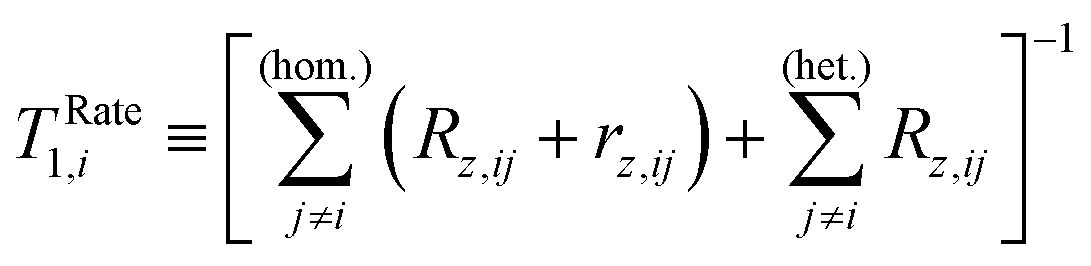The summation in each case is carried out over all spins other than i. The longitudinal auto- and cross-relaxation rates between spins i and j,respectively, depend on the autocorrelated spectral density functions J^D_ij(ω) (vide infra) of the DD interaction between the spins, evaluated at different combinations of their resonance frequencies ω_i and ω_j.⁸⁷Eqn (5) effectively treats the entire spin assembly as a network of DD-coupled two-spin systems.

2.1.2 Chemical equivalence. In NMR experiments, the chemically equivalent (CE) spins have the same resonance frequency and cannot be distinguished – only their sum magnetisation can be manipulated and observed. Using eqn (6) and (7), we get for the sum magnetisation of a pair of CE spinswhereand ω_i = ω_j = ω. We later develop the general framework for systems of any number of spins.

In the case of transverse magnetisation, we have

where S_+,i(t) = S_x,i(t) +iS_y,i(t) and . The transverse auto- and cross-relaxation rates arerespectively. At high field, transverse cross-relaxation between chemically non-equivalent (CnE) spins is suppressed by virtue of the secular approximation:^1,88 CnE spins have large differences in their resonance frequencies, due to their distinct CS values. This leads to rapidly oscillating, complex phase factors in the matrix elements of the relaxation superoperator that correspond to transverse cross-relaxation. Such matrix elements average to zero during the time evolution of the spin system, and this suppresses transverse cross-relaxation. However, similarly to the longitudinal case, transverse cross-relaxation does contribute to the observable auto-relaxation rate of the sum magnetisation of CE spins, and we havewhereThe analytic expressions of all the relaxation rates of this paper were obtained using the RELA²X programme,^87,89 and a Jupyter Notebook⁹⁰ with the necessary calculations is provided in the ESI.†

As the main interest in this work is longitudinal magnetisation dynamics and the NMR spectrum of Xe, we assume that the secular approximation holds between all CnE protons and, therefore, neglect transverse cross-relaxation between them.

2.1.3 Traditional MD–DD modelling. Conventionally one assumes all homonuclear spins (of the same isotopic type), e.g., protons, to be chemically equivalent to the extent that the analytic formulae for the relaxation rates in eqn (9) and (14) are applicable, but with each pair of spins ij having their own J_ij(ω), as governed by their internuclear dynamics. Heteronuclear (different isotopic type) relaxation is, then, computed using eqn (6), neglecting cross-relaxation. This means that, in this approximation, each spin is relaxed by all the other spins, but still evolves independently. The resulting decay is single-exponential, and is characterised by the following longitudinal and transverse relaxation times:respectively. Here, the summations are over the homo- and heteronuclear pairs, as indicated. For T₂, this can produce good results, because the transverse cross-relaxation between the CnE spins is suppressed, as noted above. The situation is different for T₁, since all mutually homonuclear spins are assumed to be chemically equivalent. Consequently, this method only works for such NMR relaxation experiments where hard inversion pulses over the entire CS range of the given isotope, which flip all spins of the same isotopic type from thermal equilibrium, are used. The traditional approach can complicate the comparison between experimental and computational T₁ results for the following reasons:

(1) The homonuclear contribution to eqn (15) is strictly speaking only valid for a system of CE spins (such as water protons), and cannot be easily justified using eqn (5) for a general system including CnE spins. In reality, the time evolution between CnE spins is coupled by cross-relaxation and, hence, deviates from the single-exponential decay.

(2) The network of nuclei coupled by cross-relaxation results in polarisation transfer and spin diffusion across the entire spin system, which can become important in large systems and/or in the presence of spin-dense solvents, such as H₂O. The traditional approach cannot describe these phenomena.

(3) Even though the experimentally measured magnetisation decay often is approximately single-exponential, due to the presence of cross-relaxation, it does, in fact, arise from coupled time evolution that inherently is not single-exponential. Therefore, the parameter that is obtained from experiments using (typically) a single-exponential fit to the decay, denoted as T^Fit₁ is, in reality, influenced by cross-relaxation. Hence, the parameters obtained from experimental data are results of fitting, whereas those extracted from traditional MD–DD modelling [eqn (15)] are inverses of self-relaxation rates. In general, the two are not the same quantity, T^Rate₁ ≠ T^Fit₁.

If the longitudinal cross-relaxation between the CnE spin groups were negligibly small, e.g., due to very weak DD couplings, the above issues (1–3) regarding T₁ would also disappear, but this is not in general the case. In the traditional MD–DD approach, it is also fairly common to neglect intermolecular relaxation, i.e., the terms where the spins i and j belong to different molecules.

Instead of neglecting longitudinal cross-relaxation, in the present work we compute all intra- and intermolecular auto- and cross-relaxation rates from MD trajectories, and simulate in full detail a physically motivated and computationally manageable version of eqn (5). This is done by formally dividing the spin system into groups of CE nuclei, with the details elaborated below. Once cross-relaxation is included, no simple analytical relationship between T₁ and the relaxation rates exists.

2.1.4 New MD–DD modelling. We now present a system of differential equations that govern the time evolution of the experimentally observable sum magnetisation of CE groups of spins. In the present context, chemical equivalence implies identical evolution under eqn (5). This establishes a close connection with experiments by using as the dynamic variable the quantity that can be experimentally manipulated and measured.

Let us formally divide the spin system into groups of chemically equivalent nuclei {I}, for which

R_z,ij ≡ R_z,IJ, ∀i ∈ I and j ∈ J

r_z,ij ≡ r_z,IJ, ∀i ∈ I and j∈J.

We then define the sum magnetisation of all S_z,i(t) within I aswhere N_I is the number of spins in group I, and the equality follows from the requirement that all CE spins have identical time evolution. Starting from eqn (5), a system of differential equations can now be derived for each M_z,I(t):The intermediate steps in the derivation are shown in the ESI.† Here,

R^CE_z,I = (N_I − 1)(R_z,II + r_z,II)

and the summation in the latter formula is carried out over all groups J other than I.

Eqn (18) generalises the traditional MD–DD approach. Each term therein has a clear interpretation: R^CE_z,I is the contribution to the observable auto-relaxation rate of M_I(t) from the DD interactions (N_I − 1 being their number) of a single nucleus within the group I of CE nuclei, and is computed according to eqn (9). R^CnE_z,I is the contribution to the auto-relaxation rate from the CnE nuclei of the other groups J ≠ I in the spin assembly, and is computed using eqn (6). The last term, which in the traditional MD–DD approach is implicitly neglected, represents the longitudinal cross-relaxation between the CnE groups, computed according to eqn (7). For a system of just two CE spins, there is only one group I, N_I = 2, and eqn (8) would be recovered. For two CnE nuclei, there are two groups I and J with N_I = 1 in both, which leads to eqn (4).

An exactly analogous derivation for the transverse magnetisation leads to

where cross-relaxation between CnE groups is suppressed by the secular approximation, and

R^CE_+,I = (N_I − 1)(R_+,II + r_+,II)

are calculated using eqn (14) and (11), respectively.Eqn (18) reduces to a differential equation for the single-exponential decay of ΔM_z,I(t), provided that one approximates that all ΔM_z,J(t) ≈ ΔM_z,I(t). In this case, the decay of ΔM_z,I(t) is described by the traditional MD–DD formulas (15) and (16). This is only true if the spin groups I and J do indeed have very similar time evolution and/or the cross-relaxation r_z,IJ between them is negligible. Later we show that the deviation between the relaxation times predicted by the simulations using eqn (18), and those using the traditional formulae, can be significant. This situation prevails for spin groups that have strong cross-relaxation to other CnE groups and do not evolve identically. In the transverse case, due to the absence of cross-relaxation between the CnE spins, the present and the traditional methods remain identical.

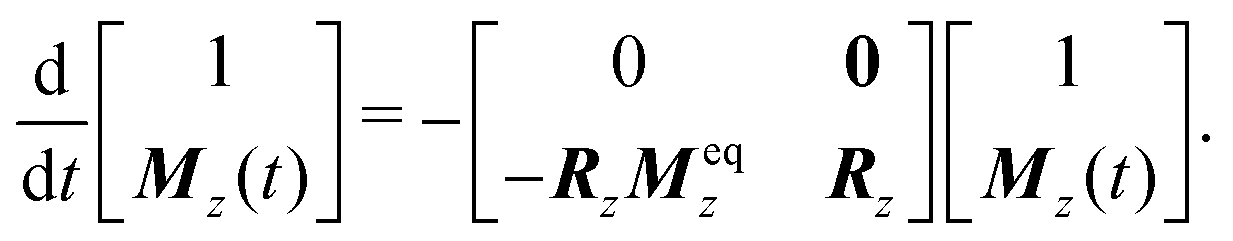
The system of eqn (18) can be cast into matrix form as

or, equivalently,where K is the total number of spin groups and we denote r_z,IJ = r_z,JI. The grouping procedure renders the array dimensions associated with eqn (21) much smaller than when eqn (5) would have been used directly, i.e., without grouping. This enables fast simulations of large spin systems over long periods of time on a standard laptop computer.

Eqn (21) is still inhomogenous and cannot be solved directly. It can, however, be effectively homogenised by adding one extra dimension to the matrix equation:

whereThe prime stands for the homogenised versions of the original matrix and vector. With a given initial condition, M_z(0), the solution to the differential equation then readsDifferent initial states M_z(0) realise standard NMR relaxation measurements for the longitudinal magnetisation, such as the inversion recovery (IR) experiment. In that context, the present framework allows modelling both hard and selective inversion pulses.

Simulated direct time propagation of M_z(t) allows the magnetisation decay to be fitted, which corresponds to extracting T^Fit₁ rather than T^Rate₁. This establishes a more justified comparison between experimental and computational results, as now both parties are referring to the same quantity, and include cross-relaxation effects in both cases. The present method implied by eqn (18) also enables simulations of polarisation transfer including spin diffusion. Furthermore, hyperpolarisation can be easily taken into account in the initial condition.

2.1.5 NOE and SPINOE enhancement. Let us then look at a model that is used to interpret SPINOE experiments in a two-spin system (spins i and j). As a result of cross relaxation-mediated polarisation transfer from spin j, the extrema (maximum or minimum) or steady-state of the magnetisation of spin i is reached when . The NOE enhancement of spin i at such a time, t₀, is defined asand, using eqn (4), we getThere are two interesting cases of eqn (26) that can be analytically studied:

(1) In the usual NOE context, the spin j is irradiated by an external radio-frequency field that depletes its spin polarisation. Then, S_z,j(t) = 0 and ΔS_z,j(t) = −S^eq_z,j. In this situation, the system reaches a steady state, where

Using the high-temperature approximation for S^eq_z and restricting our attention to spin-1/2 nuclei, we get
Here, η_ij is called the NOE enhancement factor of spin i coupled to spin j, and γ_i is the gyromagnetic ratio of i. We see that a strong cross-relaxation rate does not necessarily lead to a strong NOE enhancement, because η_ij can be suppressed by a high self-relaxation rate of spin i. The sign of η_ij depends on the ratio .

The above expression holds for a two-spin system. To take into account the presence of other spins that also contribute to the relaxation of spin i, it is common to replace R_z,i by the inverse of the experimentally obtained relaxation time T_1,i, which in the traditional computational MD–DD framework corresponds to T^Rate_1,i:

(2) The second interesting case is when spin j is hyperpolarised and relaxes relatively slowly, such that, for t ≤ t₀, we have R_z,jΔS_z,j(t) ≫ r_z,ijΔS_z,i(t), in eqn (5). We then obtain

ΔS_z,j(t₀) ≈ ΔS_z,j(0)e^−R_z,jt₀ = (ε − 1)S^eq_z,je^−R_z,j.

Here, ε is the hyperpolarisation enhancement factor of spin j, S_z,j(0) = εS^eq_z,j. The SPINOE enhancement of spin i in the presence of such a slowly relaxing, hp spin j is, therefore,where we have again accounted for the presence of other spins in the system, which contribute to the relaxation of spin j. We will refer to these two-spin models that consider the presence of other spins by adjusting the relaxation rates as “pseudo two-spin models”.

Interpretation of Xe-proton SPINOE experiments has most often used eqn (27) or formulas derived from it ref. 6, because Xe relaxation is typically much slower than that of protons by more than an order of magnitude (vide infra). However, this neglects the effects of spin diffusion, which cannot be described by a two-spin model, even when using the empirical replacement for the relaxation rate. We will later in the paper compare simulated proton SPINOE enhancements that include spin diffusion with the results predicted by eqn (27).

2.2 Relaxation-rate constants

2.2.1 Molecular dynamics simulations. We now turn our attention to computing the four relaxation-rate constants, R_z,IJ, r_z,IJ, R_+,IJ and r_+,IJ, between the different spin groups using MD simulations. First, in order to compute the rates between each spin, the spectral density functions J^D_ij(ω) are needed. If one neglects dynamic frequency shifts, J^D_ij(ω) equals the one-sided cosine transform⁸⁷Here, G^D_ij(τ) is the time-correlation function (TCF) of the rank-2, component 0 irreducible spherical tensor of the DD coupling between spins i and j:

G^D_ij(τ) = 〈V^D_ij(t)V^D_ij(t − τ)〉,

where
θ_ij(t) is the angle between the vector connecting the two spins and the external magnetic field direction (the z axis). Note that, in the present work, the approximation r_ij³(t) ≈ r_ij³ appropriate to the rigid rotor model is not used. Instead, the dynamically varying distance between the nuclei is taken into account. This is particularly important for the non-covalently bound ¹²⁹Xe spin, which samples a range of distances to other spins.

In the present MD–DD framework we work with spin groups, and the natural way to compute the relaxation rates is to take the double average over each spin in the groups i ∈ I and j ∈ J, such that and similarly for the other rates. Due to the finite length and system size (number of atoms) in a MD simulation, however, V^D_ij(τ) for a single nuclear pair ij can be quite noisy. Consequently, their cosine transforms, which would yield the spectral density functions and, eventually, the resulting relaxation rates, are often rendered unfeasible. Instead, the averaging can be carried out in the “grouped” basis, i.e.,

wherePerforming the average at the level of the grouped TCFs is computationally attractive as, with sufficient length of the MD trajectory and number of unique spin pairs in the groups I and J, the resulting TCFs G^D_IJ(τ) can have relatively little noise.

Exponentially decaying functions can be fitted to the numerical TCFs, followed by the cosine transform performed analytically. Here, we choose to use the commonly employed Lipari–Szabo double-exponential model,⁹¹ which can describe a relatively broad range of different motions. The model is a simple three-parameter fit

where the notation [ ]_IJ means that each pair IJ obtains its own fitted parameters S², τ_g and τ_e. In the present context this is primarily a convenient analytical form for the fitting function, but we will later interpret the average global correlation time τ_g between Xe and the cage protons as the rotational correlation time of the cage. Using eqn (29), we then get

The final thing we need is the G^D_IJ(0) factor, which corresponds to the mean-square amplitude of the DD coupling between spins in groups I and J. For that one has to evaluate the ensemble averages

for all i ∈ I and j ∈ J. Taken that the internuclear distances are uncorrelated with the angles, which is a reasonable assumption for ordinary isotropic liquid-state systems, the angular part can be integrated analytically to yield
In the above-mentioned rigid-rotor model one would approximate . However, this assumption needs not be made, whenever detailed MD simulations are available. The ensemble average is related to the radial distribution function (RDF),⁹²g_ij(r), between the spins i and j:where V is the volume of the system. We then defineExtracting the RDF from the MD trajectory is a routine task, after which the integral in eqn (33) can be computed numerically. In practice, the asymptotic limit R → ∞ of the integral is, e.g., for the present XBS systems, reached at roughly R = 7 Å. Hence, it can be important to be able to simulate a thick enough layer of solvent around the studied molecule, especially in cases where the solvent is expected to affect the relaxation dynamics.

Combining all of the above, the final expression for the spectral density functions J^D_IJ(ω), which is used to compute the relaxation rate constants R_z,IJ, r_z,IJ, R_+,IJ, and r_+,IJ in the present work, is

2.3 Chemical exchange

2.3.1 Two-site exchange model. Computing the relaxation rates in the different sites involved in mutual chemical exchange paves way for combining relaxation and exchange, in MD–DD modelling. Let us denote by f the free Xe atoms in the water solvent. The bound site b represents the Xe@Cage complexes. From the point of view of Xe, we can describe this as a two-state system with the rate equationwhere the relative populations of the two sites are given byHere, [n] denotes the concentration of the site n. At equilibrium, the principle of detailed balance holds:

p_fν^eq₊ = p_bν^eq₋. (38)

The chemical equilibrium state is, according to eqn (38), described by the stationary point of the differential equation for the vector P(t) = [p_f(t), p_b(t)]^T of the relative populations (concentrations):From the point of view of populations “nothing happens” in the chemical equilibrium. However, each exchanging site n is associated with a macroscopic nuclear spin state described by the magnetisation vector M⁽ⁿ⁾(t), which in NMR experiments is deliberately deviated from the equilibrium. To describe the combined evolution of both the populations and nuclear magnetisation, we assume that chemical processes are independent of the nuclear spin states, which is practically always true.

We then define the population-weighted magnetisation vector as

O(t) = P(t)⊙M(t).

where ⊙ is the Hadamard (elementwise, O_ε = P_εM_ε) product and M(t) = [M^(f)(t), M^(b)(t)]^T. The equation of motion for the longitudinal magnetisation dynamics, including chemical exchange in the two-site system, eqn (36), can then be obtained using the product rule of differentiation (details in the ESI†):Here, 1 is a unit matrix of the same dimension as R⁽ⁿ⁾_z. It is seen that chemical exchange intermixes the longitudinal relaxation dynamics of the free and bound Xe sites. Magnetisation transfer between nuclei via cross-relaxation is therefore also affected by the exchange.

Longitudinal magnetisation does not evolve under the coherent interactions, but in the transverse case we need to account for the coherent time evolution of Xe caused by the nuclear shielding interaction:

The resonance frequencies ω correspond to the Xe CS in the two different environments. The resulting trajectory of O^(f)₊(t) + O^(b)₊(t) corresponding to the NMR signal can be Fourier-transformed to obtain the ¹²⁹Xe NMR spectrum.

2.3.2 Multiscale modelling. As a final methodological note, eqn (40) and (41) realise a multiscale modelling paradigm for nuclear spin magnetisation affected by both relaxation and chemical exchange:

(1) The motionally averaged chemical shifts in ω are obtained by combining MD simulations and quantum-chemical electronic-structure calculations (see Computational details).

(2) The MD simulations allow detailed computation of the (DD) relaxation-rate constants in R, as well as (in some cases) reaction rates in ν.

(3) Magnetisation dynamics simulations combine the previous parameters into the time propagation of the appropriate observables, allowing computational spectroscopy.

3 Computational details

3.1.1 MD simulations and chemical shift calculations

Molecular dynamics simulations were performed on the xTB programme.⁹³ The three different systems, Xe(aq), Xe@3AC(aq) and Xe@6AC(aq), were simulated at the partially polarisable GFN-FF⁹⁴ force-field level of theory because of its good performance in earlier work.^47,95,96 The simulations were performed at constant temperature of 293.15 K, using the Berendsen thermostat,⁹⁷ a time step Δt = 1.0 fs and a finite droplet model with 1000 or 500 solvent H₂O molecules for the Xe(aq) or Xe@3AC/6AC(aq) systems, respectively. A weak confinement potential was used to keep the volume of the droplet approximately constant. For the Xe(aq) system a single production period of 1.8 ns was simulated, whereas for the Xe@3AC/6AC(aq) systems three independent simulations, each of 8…9 ns production period, were carried out. Snapshots were recorded every 0.1 ps.

In our previous work,⁹⁵ using similarly obtained MD trajectories, the dynamically averaged NMR chemical shifts of ¹²⁹Xe(aq) and ¹²⁹Xe@6AC(aq) were computed on the Turbomole programme^98,99 at the X2C^100,101 scalar-relativistic density-functional theory level using the BHandHLYP^102–104 exchange–correlation functional. Extensive details of the CS calculations are described in ref. 95.

3.1.2 MD trajectory analysis and DD time-correlation functions

The MD trajectory analysis, including the RDF and TCF computations, were performed using in-house written Python programmes that build upon the NumPy,¹⁰⁵ SciPy¹⁰⁶ and Numba¹⁰⁷ Python libraries. Starting from the MD trajectories, computing the full set of RDFs using a single AMD Ryzen 7 PRO processor on a standard laptop computer took roughly half an hour for each presently modelled system, and 2–3 hours for the TCFs. After the TCFs were obtained, they were fitted to the functional form of eqn (31). The computed TCFs and the fits are shown in the ESI† (Fig. S1–S3). The obtained parameters and the RDFs were used to compute the spectral density functions using eqn (35). The auto- and cross-relaxation rates between each group were then obtained according to eqn (6), (7), (9), (11), (12) and (14). Standard magnetic field of B₀ = 9.4 T was used.

The resulting longitudinal relaxation matrices, −R_z, for the Xe@Cr(aq) systems, with and without the intermolecular contributions from the solvent H₂O molecules, are shown in Fig. 2.

Fig. 2 Longitudinal relaxation matrices, −R_z, for the Xe@Cr(aq) systems (in s⁻¹). Intra- and intermolecular (the water solvent) contributions are compared. The values “0.00” correspond to matrix elements with magnitude less than 0.005. The used spin grouping is defined in Fig. 3.

3.1.3 Spin groups and magnetisation dynamics

The presently used division of the Cr cage protons into CE groups is shown in Fig. 3. Due to computational limitations (MD trajectory length), all protons of the CH₂ COOH arms were grouped together although they are not exactly equivalent. This rendered the number of spins in each group large enough for gaining sufficient statistics for G^D_IJ(τ). Protons in the solvent water pool were taken as one spin group in each case.

Fig. 3 Division of the Cr cage protons into spin groups. The number of spins in each group is shown. Note that the 3AC cage is divided into five groups, and the 6AC cage into four.

Time propagation of eqn (24) and the analysis of the results were carried out on in-house written programmes using the Python and Jupyter Notebook⁹⁰ environments. To extract T^Fit₁ from the simulated magnetisation decay we used the following single-parameter fit

which corresponds to how T₁ is extracted in experiments. The magnitude of the NOE/SPINOE polarisation transfer was in eqn (25) and (27) defined as the maximum of S_z(t), which occurs when t = t₀. Hence, the simulated maximum polarisation transfer for each group I was also extracted as

3.1.4 Chemical exchange

The equilibrium exchange-rate constants ν^eq_± are presently the only parameters that had to be obtained using experimental data. Their computation is very difficult because the Xe exchange events are extremely rare in the MD simulation time scale. Hence, gaining statistically trustworthy computational values for ν^eq_± was considered to lie outside the scope of the current computational methodology. The actual parameter that was taken from experiments is K_a = 6800 M⁻¹ for Xe@6AC in D₂O, as reported in ref. 48. The input parameters for the simulations are the initial concentrations [Xe]_init and [Cage]_init, which were here chosen to be equal to obtain comparable peak intensities in the ¹²⁹Xe NMR spectrum. We then solve for [Xe@Cage]_eq using eqn (3) with

[Xe]_eq = [Xe]_init − [Xe@Cage]_eq

[Cage]_eq = [Cage]_init − [Xe@Cage]_eq,

as detailed in the ESI.† In the language of the two-site model, the concentrations of the free site f and the bound site b are

[f] = [Xe]_eq and [b] = [Xe@Cage]_eq.

Using eqn (37), this leads to p_f = 0.32 and p_b = 0.68. With ν_ex, which is taken to be the central control variable in the present series of simulations, using eqn (38) one can then solve for the equilibrium exchange rates as

4 Results and discussion

4.1 Relaxation times of the free and bound sites

First we survey the results obtained in the absence of chemical exchange. Table 1 shows the longitudinal relaxation times and the NOE/SPINOE enhancements of each spin resulting from different initial states M_z(0), which correspond to different inversion recovery experiments. The traditional MD–DD approach (T^Rate₁), the presently introduced method (T^Fit₁), as well as the simulated SPINOE enhancement and the enhancement predicted by the pseudo two-spin model of eqn (27), are compared. The transverse relaxation times T^Rate₂ are also shown.

Table 1 Simulated longitudinal (T₁) and transverse (T₂) relaxation times and NOE/SPINOE enhancements for the free Xe(aq), Xe@3AC(aq) and Xe@6AC(aq) systems. Results starting from different initial states M_z(0) are shown. In the case of longitudinal relaxation, the traditional approach (T^Rate₁) is compared with the presently introduced method (T^Fit₁). The simulated SPINOE enhancement is compared with prediction of the pseudo two-spin model of eqn (27). The time t₀ is when the SPINOE maximum is reached. Chemical exchange effects are not yet included in these data

System	M z (0)^a	Property	^129Xe	^1H linker	^1H aromatic	^1H axial	^1H acid	^1H methoxy	^1H water
a Specifies the inverted (ε = −1) or hyperpolarised (by a factor of 1000, ε = 1000) nuclei. εH denotes an initial nonequilibrium state for all protons, whereas εH(xAC) means that only the cage protons were in a nonequilibrium initial state.
Xe(aq)		T ^Rate1 (s)	138.53	–	–	–	–	–	6.53
		T ^Rate2 (s)	138.63	–	–	–	–	–	6.53
	ε Xe = 1000	T ^Fit1 (s)	138.53	–	–	–	–	–	6.53
		t 0 (s)	–	–	–	–	–	–	20.93
		SPINOE(t0) [%]	–	–	–	–	–	–	0.28
		SPINOE(t0), eqn (27) [%]	–	–	–	–	–	–	0.28
	ε H = −1	T ^Fit1 (s)	–	–	–	–	–	–	6.53
		t 0 (s)	20.93	–	–	–	–	–	–
		NOE(t0) [%]	−14.59	–	–	–	–	–	–
Xe@3AC(aq)		T ^Rate1 (s)	16.89	0.52	1.14	0.61	0.85	1.24	6.3
		T ^Rate2 (s)	12.86	0.09	0.26	0.04	0.51	0.52	6.3
	ε Xe = 1000	T ^Fit1 (s)	16.89	–	–	–	–	–	–
		t 0 (s)	–	2.22	3.15	3.34	2.99	4.13	8.96
		SPINOE(t0) [%]	–	7.62	12.76	4.75	5.84	5.79	0.22
		SPINOE(t0), eqn (27) [%]	–	6.91	13.12	2.24	4.96	4.04	0.38
	ε H(3AC) = −1	T ^Fit1 (s)	–	0.59	1.28	0.85	0.98	1.51	–
		t 0 (s)	3.14	–	–	–	–	–	2.3
		NOE(t0) [%]	−10.39	–	–	–	–	–	0.61
	ε H = −1	T ^Fit1 (s)	–	0.52	1.03	0.74	0.8	1.21	6.29
		t 0 (s)	4.51	–	–	–	–	–	–
		NOE(t0) [%]	−14.96	–	–	–	–	–	–
Xe@6AC(aq)		T ^Rate1 (s)	17.08	0.47	1.16	0.68	0.78	–	6.07
		T ^Rate2 (s)	12.24	0.09	0.22	0.04	0.3	–	6.07
	ε Xe = 1000	T ^Fit1 (s)	17.08	–	–	–	–	–	–
		t 0 (s)	–	2.27	3.15	3.62	3.12	–	8.97
		SPINOE(t0) [%]	–	5.85	12.06	5.48	4.55	–	0.24
		SPINOE(t0), eqn (27) [%]	–	5.03	13.16	2.16	3.31	–	0.38
	ε H(6AC) = −1	T ^Fit1 (s)	–	0.55	1.32	1.06	0.95	–	–
		t 0 (s)	3.12	–	–	–	–	–	2.18
		NOE(t0) [%]	−9.31	–	–	–	–	–	0.63
	ε H = − 1	T ^Fit1 (s)	–	0.48	1.06	0.89	0.78	–	6.06
		t 0 (s)	4.83	–	–	–	–	–	–
		NOE(t0) [%]	−14.32	–	–	–	–	–	–

---

4.1.1 Relaxation of ¹²⁹Xe. Let us first look at the relaxation of ¹²⁹Xe in the free and host-bound environments. The simulated longitudinal magnetisation decay starting from a hyperpolarised initial state with ε_Xe = 1000, is plotted in Fig. 4 [relaxation of Xe was found practically independent of the initial polarisation, so we use the same ε_Xe = 1000 simulation to discuss both Xe relaxation and the polarisation transfer to the surrounding protons (vide infra)]. We see that T₁ is of the order of 10¹…10² s in all the presently considered environments, i.e., relaxation is relatively slow as compared to, e.g., typical proton relaxation, with T₁ of the order of 10⁻¹…10⁰ s. This is because no other atoms are covalently bound to the noble gas atom, which renders the average internuclear Xe-proton distances relatively high and, hence, weakens the DD relaxation. The rapid rotational tumbling of H₂O molecules around the free Xe in solution is less effective in causing relaxation as compared to the slower tumbling of the Cr cages (see below), and this is reflected in the decay profiles.

Fig. 4 Longitudinal magnetisation decay of the free and host-bound ¹²⁹Xe sites starting from a state with ε_Xe = 1000.

Relaxation of Xe in each environment is characterised by the relaxation times shown in Table 1. The computed free-Xe T₁ is 138.53 s, whereas for Xe@3AC and Xe@6AC, it is much shorter, 16.89 and 17.08 s, respectively. Notably, the relaxation of Xe in water is very slow with a T₁ of more than two minutes. The difference between the T₁ values of the two kinds of bound sites is very small, roughly 0.2 s. For both of them, a substantial contribution, roughly 20%, of the encapsulated Xe relaxation-rate values comes from the intermolecular relaxation caused by the water solvent (see the longitudinal relaxation matrices in Fig. 2). In all cases the traditional (T^Rate₁) and the presently used method (T^Fit₁) produce identical results for ¹²⁹Xe. This is because of the relatively weak cross-relaxation between Xe and the surrounding protons, resulting from the weak Xe-proton DD couplings.

Transverse relaxation times T^Rate₂ of 138.63, 12.86 and 12.24 s were obtained for the free, Xe@3AC and Xe@6AC sites, respectively. T₁ and T₂ are nearly equivalent for the free site. This is a feature of a slow relaxation caused by rapid rotational tumbling, which is precisely the situation due to the water molecules around the free xenon. The difference between T₁ and T₂ becomes more pronounced for the bound Xe sites, where the computed T₂ values are smaller than T₁ by roughly 4… 5 s. The average τ_g values [see eqn (31)] obtained from the DD-TCF fits between Xe and the cage protons are 1.38 and 1.48 ns for the Xe@3AC and Xe@6AC systems, respectively. These values can be interpreted as due to the relatively slow rotation of the Cr cages. This, in turn, renders the relative contribution of the zero-frequency spectral density function J(0) in the expression for the transverse relaxation rate [eqn (11)] much larger than in the case of the rapidly tumbling H₂O molecules, which rationalises the difference from Xe(aq). For comparison, a much faster rotational correlation time of 0.6 ns was experimentally found for a prototypic (0AC) cryptophane-A cage dissolved in deuterated tetrachloroethane (C₂D₂Cl₄).⁸⁰ The water-soluble 3AC and 6AC cages carry the CH₂COOH acetic acid groups [see Fig. 1], which are longer than the six methoxy (CH₃) groups of the 0AC cage, extend further into the bulk solvent, and hydrogen-bond with the water molecules. Hence, the CH₂COOH groups can be expected to slow down the rotation of the 3AC and 6AC cages, as seen in the MD simulations.

The presently computed longitudinal relaxation time for Xe(aq), T₁ = 138.53 s, is in an excellent agreement with the previous experimental result of 137 ± 4 s at 293 K,¹⁷ albeit in that work also other relaxation mechanisms were reported to affect the experimental value. For the Xe@3AC and Xe@6AC systems, no directly comparable experimental data are available, but the T₁ values of 16 s for Xe@0AC in C₂D₂Cl₄ at 295 K⁸⁰ and 12 s for Xe@6AC in D₂O at 293 K, at a magnetic field of B₀ = 11.7 T,⁴⁸ have been reported. The present simulations predict somewhat slower relaxation of Xe than in these experiments. We suspect that the confinement potential used in the present droplet-model GFN-FF MD simulations might restrict the rotational motion of the Cr cages, leading to longer rotational correlation times and, in fact, slower Xe relaxation (see Fig. S4 and discussion in the ESI†). This issue is not present in the Xe(aq) MD simulations, however. More reliable MD trajectories could be obtained by using a larger droplet model with a thicker layer of solvent around the Xe@3AC and Xe@6AC systems, or, preferably, periodic boundary conditions. Longer MD trajectories would also be desirable for gaining improved DD TCF statistics at large values of the time offset τ.

4.1.2 Relaxation of ¹H. We then turn to the relaxation of the Cr protons. Fig. 5 illustrates the simulated M_z,I(t) for the different proton groups and the exponential fits thereto, carried out using eqn (42). Two different inversion-recovery experiments were simulated, one with just the cage protons being initially inverted [ε_H(xAC) = −1] and the other with all, both cage and water protons inverted (ε_H = −1). The T₁ values obtained by the traditional MD–DD method (here including both intra- and intermolecular contributions), are compared with the values extracted from the exponential fits, in Fig. 6.

Fig. 5 Results after the inversion of the cage protons for (a) 3AC and (b) 6AC cages. Results after the inversion of all protons in the system for (c) 3AC and (d) 6AC cages.

Fig. 6 Relaxation rates of ¹H in the Xe@3AC and Xe@6AC systems. (a) and (b) T₁ obtained by different methods. (c) and (d) T^Rate₂. The core (left) and arm (right) protons are divided by the dashed black line.

All three methods predict that the 3AC and 6AC protons have a T₁ around 1 s, which is roughly an order of magnitude smaller than what was found the encapsulated ¹²⁹Xe. This is because the hydrogen atoms in the Cr cages have other hydrogens (both in the cage and the H₂O solvent) relatively near, which renders the average DD couplings stronger than in the Xe-proton case. In addition, the gyromagnetic ratio of ¹H is about a factor of four times larger than that of ¹²⁹Xe. This increases the proton relaxation rates and, hence, decreases T₁. The intermolecular relaxation of the cage protons caused by the water solvent amounts to roughly 20… 30% of the total longitudinal relaxation rate values, as shown in Fig. 2.

In the first simulated experiment in which only the cage protons are inverted, ε_H(3AC) = −1 shown in panels (a) and (b) of Fig. 5, the intramolecular relaxation of the Cr protons dominates because the water group remains close to thermal equilibrium. Apart from contributing to the self-relaxation rates, the water protons in this experiment only have a minor impact on the time evolution of the cage protons. We see that the simulated decay curves are roughly single-exponential, albeit some deviation is caused by cross-relaxation between the CnE groups.

In the second, ε_H = −1 experiment [Fig. 5(c) and (d)], also the intermolecular cross-relaxation with the water solvent becomes important. The H₂O group relaxes relatively slowly as compared to the Cr protons. All presently computed cross-relaxation rates between the cage and the water protons are negative (see Fig. 2). Consequently, after inversion, the negative total magnetisation of the water group drives, in its part, the Cr groups towards the positive equilibrium magnetisation. Hence, cross-relaxation manifests itself in the effectively faster decay towards the equilibrium and leads to a smaller value of T^Fit₁, as compared to the ε_H(xAC) = −1 simulation without water group inversion [see Table 1]. For t > 3…4 s, the inverted magnetisation of water acts as an additional source of polarisation that results in a long, positive “NOE magnetisation tail” of the cage protons.

In Fig. 6(a) and (b), we see that the T^Rate₁ values are on average closer to T^Fit₁ obtained from the ε_H = −1 simulations than to those obtained from the ε_H(xAC) = −1 simulations. This is because T^Rate₁ is calculated by summing up the contributions from all homonuclear spins [eqn (15)], which effectively assumes that all protons are inverted in the NMR experiment (vide supra), corresponding exactly to the ε_H = −1 situation. The ε_H(3AC) = −1 simulations, where the water protons are not inverted, lead to T^Fit₁ values that are systematically larger than T^Rate₁. This results from the near-absence of cross-relaxation between the cage and water protons, which would drive the cage protons towards thermal equilibrium, as discussed above.

For the linker, acid and methoxy proton groups, which have no other nearby CnE spins [Fig. 3], the T^Rate₁ values are very close to T^Fit₁ obtained from the ε_H = −1 simulations. The situation is, however, very different for the aromatic and axial protons that belong to the CTB bowls of the Cr cages. In these cases, the differing self-relaxation rates and the presence of strong mutual cross-relaxation (see Fig. 2) render the difference between the T^Rate₁ and T^Fit₁ approaches to amount to roughly 15…30%, depending on which of the two cages and which proton group is investigated. This reflects the fact that approximating ΔM_z,J(t) ≈ ΔM_z,I(t) in eqn (18), which leads to the traditional MD–DD approach, is not necessarily justified between such CnE spin groups that do not have nearly identical self-relaxation rates, and which are connected by strong cross-relaxation. Magnetisation transfer between the aromatic and axial protons is seen to effectively intermix their observable relaxation times, which tend to, in the T^Fit₁ simulations, converge towards an average of the two distinct T^Rate₁ values of these spin groups.

The simulated T₂ values, roughly 0.05…0.5 s in Fig. 6(c) and (d), are smaller than T₁ by a factor of 2…15, depending on the proton group. Similarly as in the case of ¹²⁹Xe, the J(0) term in the proton T₂ [eqn (11) and (14)], which does not appear in the corresponding T₁ expressions [eqn (6) and (9)], increases in importance due to the slow rotational tumbling of the Cr cage. The relative differences between the core and arm protons [see Fig. 3], particularly in the 3AC cage, becomes visible. This is because of their different dynamics; the slow rotation of the cage leads to a smaller value of T₂ for the core protons than for the arm protons, which undergo less restricted, more dynamic motion. In the 6AC cage, the CH₂COOH groups block each other sterically, which somewhat hinders their overall motions. This is different from the situation in the 3AC cage, where the acid protons are less restricted: the smaller methoxy groups on the opposite CTB bowl do not similarly block the mobility of the CH₂COOH arms.⁹⁶ Hence, the acid protons in 6AC are more dynamically similar to the core protons than in the 3AC cage, which leads to the predicted differences in T₂.

Experimental relaxation times of the Cr protons are only available for the longitudinal magnetisation in the Xe@0AC(C₂D₂Cl₄) system, at 295 K.⁸⁰ Therein, T₁ values of 0.39, 0.80, 0.31 and 0.83 s were measured for the linker, aromatic, axial and methoxy protons, respectively. The corresponding, presently simulated values of 0.59/0.55, 1.28/1.32, 0.85/1.06 and 1.51 s for the 3AC/6AC cages, are in an order-of-magnitude agreement with these experimental data. As discussed above, we believe that the quality of the MD simulations may contribute to this discrepancy. In addition, the different cage structures and solvents can induce significant differences in the proton relaxation dynamics. In our simulations, the rotational correlation times of the 3AC/6AC cages in H₂O (1.38 and 1.48 ns) are much larger than that measured for the 0AC cage in C₂D₂Cl₄ (0.60 ns). According to Fig. S4 (ESI†), in this correlation-time regime, the presently simulated, slower rotational dynamics corresponds to a longer T₁—precisely as we see from the simulations results for the latter quantity.

4.2 Polarisation transfer

4.2.1 SPINOE of ¹H. We turn our attention to the SPINOE polarisation transfer from the hp Xe to the surrounding protons. The time evolution of each proton group, starting from an initial state characterised by ε_Xe = 1000 [same simulation as in Fig. 4], is shown Fig. 7(a) and (b). The time t₀ when the SPINOE maximum is reached, and the corresponding SPINOE value at that time, are reported in Table 1. 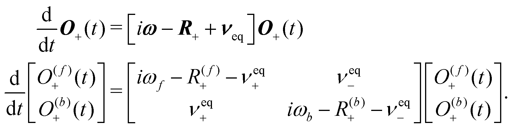The ensemble average , as in eqn (33) and (34), between Xe and each proton group, is shown in panels (c) and (d) of the Figure.

Fig. 7 (a) and (b) Transient SPINOE curves of the proton groups resulting from the presence of hyperpolarised Xe with ε_Xe = 1000. (c) and (d) [in units of Å⁻⁶] as in eqn (33) and (34). All water molecules of the simulation droplet were included in the water proton group.

Fig. 7(a) and (b) show the typical shape of a transient NOE peak, now resulting from the presence of hp Xe with ε_Xe = 1000. The maximum SPINOE enhancement of the protons is in the range of 4…13%. The maxima are reached at roughly t₀ = 2…4 s, after which the protons decay following the relaxation of ¹²⁹Xe, as is seen by comparing with Fig. 4. Inside the Cr cages, the hp Xe acts as a source of polarisation for the surrounding protons, prolonging their relaxation times as compared to the situation without Xe hyperpolarisation.

Because the Xe-proton DD couplings and the resulting cross-relaxation rates depend on the interatomic distances as 1/r⁶, the distance distribution of the protons around the encapsulated Xe is an important factor in the SPINOE transfer. Fig. 7(c) and (d) show that the values of the ensemble average (at the asymptotic limit, R_Xe–H > 7 Å) for the different proton groups are reflected in the SPINOE enhancements [panels (ab)], but do not alone determine the relative size of the latter. SPINOE is also affected by the self-relaxation rates of the protons, as was discussed in connection with eqn (27). For both Xe@3AC and Xe@6AC, the linker and aromatic protons reside on average in close proximity to the encapsulated Xe (see Fig. 1 and 3). This renders the DD couplings of the Xe-linker and Xe-aromatic pairs strong, as implied by the values. The fact that the linker protons relax much faster as compared to the aromatic protons (Fig. 6), is clearly reflected in the SPINOE peaks. Polarisation transfer to the aromatic protons is the strongest among all the proton groups, whereas that to the linker protons is clearly weaker. According to the values, in the Xe@3AC system the linker protons have on average a slightly larger DD coupling to Xe than in the Xe@6AC case. This leads to a higher SPINOE enhancement in the 3AC cage. In both systems, protons in the axial group reside far away from the xenon atom, which weakens their DD couplings and SPINOE transfer. As was discussed earlier, the acid groups of the 6AC cage extend further out into the solvent and block each other from getting close to Xe. In contrast, in the 3AC cage, the methoxy and acid protons are able to reach positions in close vicinity of xenon. These features are reflected in the and SPINOE values.

However, even considering both the average Xe-proton DD couplings and the self-relaxation rates of the proton spins, is not sufficient to understand the relative order of the individual simulated SPINOE enhancements. Yet another important mechanism, which affects the efficiency of the SPINOE transfer, is provided by the proton–proton cross-relaxation, i.e., spin diffusion. In Fig. 8, the simulated results are compared with those predicted by the pseudo two-spin model of eqn (27), where the latter neglects the proton–proton cross-relaxation. We see that for the aromatic protons, the two-spin model predicts results that are slightly higher than, but still in good agreement with the full simulations. This is because these protons on average reside relatively close to the Xe guest, such that most of their SPINOE enhancement is a result of direct DD coupling to the xenon nucleus [Fig. 7(c) and (d)]. In contrast, the linker, axial, methoxy and acid protons receive a higher SPINOE enhancement in the simulations than what eqn (27) predicts. Due to the proton–proton cross-relaxation network in the systems (see the off-diagonal elements in Fig. 2), polarisation transfer from the hp Xe is mediated by the aromatic protons, which are in strong contact with Xe and relax relatively slowly, to the faster-relaxing linker and axial protons. Then, the proton–proton cross-relaxation network conveys the polarisation to the methoxy and acid protons, as well. This is reflected in the higher SPINOE maxima predicted for these spin groups by the full simulations, which include spin diffusion effects. It can be concluded that the SPINOE polarisation transfer in the Xe@cryptophane systems is a fairly complicated process influenced by three effects: direct Xe-proton cross-relaxation, proton self-relaxation and proton–proton cross-relaxation.

Fig. 8 Maximum SPINOE transfer to the 3AC and 6AC cage protons from hyperpolarised Xe with enhancement factor ε_Xe = 1000. Simulations that account for proton–proton cross-relaxation are compared to the pseudo two-spin model of eqn (27).

The present simulations were performed at B₀ = 9.4 T. We note that, at lower magnetic fields, the proton SPINOE enhancement relative to the thermal polarisation would be much greater in magnitude. Xe hyperpolarisation factors ε_Xe exceeding the value of 1000 used in this paper can nowadays be obtained with modern SEOP setups.

4.2.2 NOE of ¹²⁹Xe. In Table 1, results for the NOE polarisation transfer to thermally polarised Xe are shown after inversion of either all or only the cage protons. The sign of the NOE transfer is always negative, which is due to the negative gyromagnetic ratio of the ¹²⁹Xe nucleus. In each system, the inversion of all protons depletes the initial Xe magnetisation by up to 15%, whereas the inversion of merely the cage protons leads to a roughly 10% depletion. Based on these results, ¹²⁹Xe NMR signal enhancement of up to 15% could be obtained in experiments of similar systems by first inverting the Xe pool followed by a proton inversion, and then waiting for t₀ = 3…21 s for the Xe polarisation to build up, before performing the actual measurement.

4.3 Effect of chemical exchange

Xenon exchange between the solution and cryptophane cage confinement is treated using the two-site model described above, in the Section Theoretical Background. The longitudinal relaxation times of ¹²⁹Xe and the SPINOE transfer to the Cr protons are studied as a function of ν_ex ranging from the situation of no exchange (ν_ex = 0) to a rapid exchange with ν_ex = 10³ s⁻¹, corresponding to a typical Xe exchange rate in Xe@Cage(aq) systems. We also simulate the ¹²⁹Xe NMR spectrum as obtained by the present multiscale modelling paradigm (see theoretical background), with the equilibrium constant K_a = 6800 M⁻¹ [experimental result for Xe@6AC(aq)⁴⁸] constituting the only empirical input. The presently computed transverse relaxation times T^Rate₂ are used, and the CS values of the free and host-bound Xe are adopted from our earlier work.⁹⁵ We restrict ourselves to the Xe@6AC system, since both the experimental K_a value and the earlier CS calculations involved the 6AC cage. As such, the present methodology can be readily applied for the Xe@3AC, or any other Xe@host system.

4.3.1 Longitudinal ¹²⁹Xe relaxation. Fig. 9 shows T^Fit₁ of ¹²⁹Xe as a function of ν_ex for the free (f) and host-bound (b) sites. At ν_ex = 0, there is no chemical exchange and the values correspond to those in Table 1. When ν_ex increases, we see that the T₁ value for the bound site increases slowly, whereas there is a rapid decrease for the free site. Because of the overall faster relaxation of the bound site, T₁ of the free site diminishes due to Xe exchange. As ν_ex increases towards 1000 s⁻¹, the two T₁ values converge to a common, population-weighted average value. The final simulation result, T₁(ν_ex = 1000 s⁻¹) = 23.3 s, is in perfect agreement with the prediction based on the analytical formula which is appropriate for exchange that is fast with respect to the relaxation times of the individual exchanging sites. Due to the relatively slow relaxation of ¹²⁹Xe, the above formula continues, in fact, to be applicable down to ν_ex ≈ 1 s⁻¹, as can be seen from Fig. 9. Note that this situation does not yet, however, correspond to fast exchange in the sense of the difference in the resonance frequencies of the two sites. We will return to this issue below, in the discussion of the ¹²⁹Xe NMR spectrum.

Fig. 9 T ^Fit₁ of ¹²⁹Xe as a function of the exchange rate ν_ex (s⁻¹) for the free (f) Xe(aq) and host-bound (b) Xe@6AC(aq) sites. The relative populations are p_f = 0.32 and p_b = 0.68.

4.3.2 ¹H SPINOE. The maximum SPINOE enhancement of the 6AC cage protons is shown in Fig. 10 as a function of ν_ex. Panel (a) compares the free and bound sites. The situation resembles that in Fig. 9: at ν_ex = 0, the SPINOE transfer only takes place within the bound site, because there is no cross-relaxation between Xe and the cage protons in the free site. As ν_ex increases, the SPINOE enhancement of the bound-site protons decreases and that of the free-site protons increases. A converged plateau is, again, reached at ν_ex = 100 s⁻¹.

Fig. 10 (a) SPINOE transfer from hp ¹²⁹Xe to the 6AC protons as a function of ν_ex for the free and host-bound sites. (b) Total SPINOE transfer.

Fig. 10(b) shows the total SPINOE transfer, equalling the sum of the free and bound sites. The total SPINOE increases with the Xe exchange rate, until the plateau at ν_ex = 100 s⁻¹ is reached. This can be understood based on the very slow relaxation of ¹²⁹Xe in the free site (T₁ = 138.53 s, see Table 1). In water solution, the hp ¹²⁹Xe retains its high magnetisation level for a long time. Through the chemical exchange, the pool of host-bound Xe spins is replenished from the free Xe pool, which, during the timescale of the SPINOE transfer (2…5 s, see t₀ values in Table 1), has not had time to relax by a substantial amount. Thus, the free site in this case acts as a long-lived “storage” of hyperpolarisation, which eventually is conveyed to the cage protons via chemical exchange. The resulting overall increase in the SPINOE transfer with ν_ex = 100 s⁻¹ amounts up to 40%, as compared to the situation with no exchange.

4.3.3 ¹²⁹Xe NMR spectrum. As a final demonstration of the present multiscale simulations, Fig. 11 shows the computational ¹²⁹Xe NMR spectra for different values of ν_ex. Starting from the top, two clearly distinguishable peaks are seen when the exchange rate is small as compared to the difference in resonance frequencies of the free and bound sites, . In this case the system is in the slow-exchange regime. The peak on the left with CS of 182 ppm corresponds to Xe(aq), and the one on the right to Xe@6AC(aq) at 67 ppm. These are the first-principles calculated shift values from ref. 95. The intensities of the peaks are proportional to the populations p_f = 0.32 and p_b = 0.68. When the exchange rate increases towards the bottom of the figure, a characteristic, asymmetric exchange broadening of the peaks takes place and a crossover occurs at ν_ex ≈ |Δω|. At this point, the exchange broadening affects the spectrum the most and the combined peak is barely visible. When ν_ex increases further, towards the fast-exchange regime a single peak at the population-weighted average CS, δ = p_fδ_f + p_bδ_b ≈ 104 ppm, is seen.

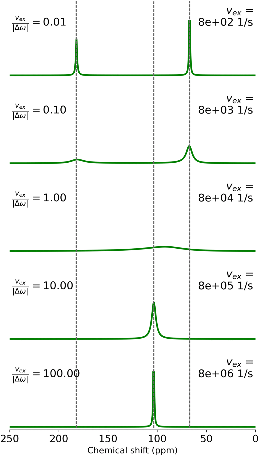Fig. 11 Simulated NMR spectra of ¹²⁹Xe exchanging between free and 6AC-bound environments for different values of exchange rate ν_ex. The dashed vertical lines indicate the computed chemical shift values of the free and bound states, as well as their population-weighted average.

5 Conclusions

Dynamic modelling of large, conformationally flexible molecules and their magnetisation dynamics remains a challenge in computational NMR. On the one hand, fully quantum-mechanical spin dynamics simulations, which incorporate relaxation effects, offer accurate insights into the behaviour of small and relatively rigid molecules. These methods face, however, scalability issues when applied to large molecular systems and/or cases requiring intermolecular relaxation, such as in aqueous solvation environments of relevance to biological applications. On the other hand, molecular dynamics simulations have been used to model particularly the dipole–dipole relaxation in scenarios where full spin dynamics simulations have been unfeasible. Unfortunately the traditional MD–DD approaches have typically neglected cross-relaxation effects, which are responsible for the NOE polarisation transfer, between chemically non-equivalent spin groups. This limitation has complicated direct comparison between experimentally determined relaxation rates and those derived from MD–DD simulations.

This work bridges the methodological gap between fully quantum-mechanical spin dynamics simulations and conventional MD–DD methods. We have developed new multiscale modelling techniques for simulating the longitudinal relaxation dynamics in large, flexible molecular systems. Specifically, we improved upon traditional MD–DD modelling by incorporating cross-relaxation effects and directly propagating the equations of motion for the magnetisation observables. This also facilitates the inclusion of chemical exchange processes in relaxation modelling across arbitrary exchange rate regimes. The newly developed methods enable simulation of not only relaxation but also that of polarisation transfer among spins and between the chemically exchanging sites.

Computational feasibility was achieved by partitioning a large spin system into groups of chemically equivalent nuclei, allowing fast simulations on a standard laptop computer. Starting from the Solomon equations, we derived a set of differential equations that generalise the conventional MD–DD approach for spin systems including chemically non-equivalent nuclei, maintaining rigour in the expressions of the spectral densities involving two different spin groups, and presented the computational approach for determining DD relaxation rates between the spin groups and simulating their time evolution.

The developed methods were applied to examine longitudinal magnetisation dynamics in three model systems pertinent to the field of ¹²⁹Xe NMR biosensors: Xe(aq), Xe@3AC(aq) and Xe@6AC(aq), where 3AC and 6AC are water-soluble derivatives of cryptophane-A. In these Xe@host systems, Xe hyperpolarisation, DD relaxation, and Xe exchange are interdependent, and the present methods enable their simultaneous modelling. Additionally, the ¹²⁹Xe NMR spectrum was simulated under various exchange conditions. Xe and proton relaxation times, NOE and SPINOE polarisation transfer, and the impact of chemical exchange on these features, were reported. This work establishes a foundation for studying DD relaxation and cross relaxation-mediated polarisation transfer across diverse molecular systems, including those in non-deuterated solvents. Our principal message is that the analysis methodology introduced here is highly general and allows for systematic and theoretically consistent generation of computational data for direct comparison with experiments, provided that carefully calibrated MD force fields are employed and sufficient statistics is reached. The rigorous analysis of the magnetisation dynamics data may, in turn, also aid in the development of the force fields. The present capability for relaxation modelling opens up new avenues for studying Xe@host systems, complementing existing work focused on Xe chemical shifts as means of achieving chemical resolution in sensor applications. We hope that these advances in modelling relaxation and Xe-proton SPINOE experiments will foster new experimental studies in the field, including those involving selective inversion-recovery pulses and/or combined ¹H and ¹²⁹Xe pulse sequences.

Author contributions

P. Hilla was responsible for data curation, general investigation, software coding, visualisation of methods and results, and writing of the original draft; J. Vaara supervised the entire work. Both authors contributed together to conceptualisation of the project and reviewing/editing of the manuscript.

Data availbility

The Rela2x Jupyter Notebook file supporting this article has been included as part of the ESI.†

Conflicts of interest

There are no conflicts to declare.

Acknowledgements

Joni Eronen, Pau Mayorga Delgado, Anu Kantola and Ville-Veikko Telkki (Oulu) are thanked for many useful discussions. Funding from Jenny and Antti Wihuri foundation and the University of Oulu Graduate School is appreciated (P. H.). We acknowledge funding from the Academy of Finland (grants 331008 and 361326) and U. Oulu (Kvantum Institute).

Notes and references

1. J. Kowalewski and L. Mäler, Nuclear Spin Relaxation in Liquids, CRC Press, 2nd edn, 2018.
2. A. W. Overhauser, Phys. Rev., 1953, 92, 411–415.
3. G. Navon, Y. Song, T. Rom, S. Appelt, R. E. Taylor and A. Pines, Science, 1996, 271, 1848–1850.
4. Y. Song, B. M. Goodson, R. E. Taylor, D. D. Laws, G. Navon and A. Pines, Angew. Chem., Int. Ed. Engl., 1997, 36, 2368–2370.
5. T. Pietraß, Colloids Surf., 1999, 158, 51–57.
6. Y.-Q. Song, Concepts Magn. Reson., 2000, 12, 6–20.
7. G. Lippens, D. van Belle, S. J. Wodak and J. Jeener, Mol. Phys., 1993, 80, 1469–1484.
8. M. Odelius, A. Laaksonen, M. H. Levitt and J. Kowalewski, J. Magn. Reson., Ser. A, 1993, 105, 289–294.
9. M. Luhmer, A. Moschos and J. Reisse, J. Magn. Reson., Ser. A, 1995, 113, 164–168.
10. C. Peter, X. Daura and W. F. van Gunsteren, J. Biomol. NMR, 2001, 20, 297–310.
11. J.-P. Grivet, J. Chem. Phys., 2005, 123, 034503.
12. J. T. Gerig, Mol. Simul., 2012, 38, 1085–1093.
13. P. M. Singer, D. Asthagiri, W. G. Chapman and G. J. Hirasaki, J. Magn. Reson., 2017, 277, 15–24.
14. A. Philips and J. Autschbach, Phys. Chem. Chem. Phys., 2019, 21, 26621–26629.
15. D. Asthagiri, W. G. Chapman, G. J. Hirasaki and P. M. Singer, J. Phys. Chem. B, 2020, 142, 10802–10810.
16. P. S. Hubbard, Phys. Rev., 1963, 131, 275–282.
17. I. E. Dimitrov, R. Reddy and J. S. Leigh, J. Magn. Reson., 2000, 145, 302–306.
18. M. Gerken and G. J. Schrobilgen, Coord. Chem. Rev., 2000, 197, 335–395.
19. B. Goodson, J. Magn. Reson., 2002, 155, 157–216.
20. A.-M. Oros and N. J. Shah, Phys. Med. Biol., 2004, 49, 105–153.
21. D. Raftery, Annu. Rep. NMR Spectrosc., 2006, 57, 206–261.
22. K. Bartik, M. Luhmer, J.-P. Dutasta, A. Collet and J. Reisse, J. Am. Chem. Soc., 1998, 120, 784–791.
23. T. Brotin and J.-P. Dutasta, Chem. Rev., 2009, 109, 88–130.
24. G. El-Ayle and K. Travis, Comprehensive Supramolecular Chemistry II, Elsevier, 2017, pp. 199–249.
25. T. Walker and W. Happer, Rev. Mod. Phys., 1997, 69, 629–642.
26. J. Eills, D. Budker, S. Cavagnero, E. Y. Chekmenev, S. J. Elliott, S. Jannin, A. Lesage, J. Matysik, T. Meersmann and T. Prisner, et al. , Chem. Rev., 2023, 123, 1417–1551.
27. A. Cherubini and A. Bifone, Prog. Nucl. Magn. Reson. Spectrosc., 2003, 42, 1–30.
28. B. Driehuys, Science, 2006, 314, 432–433.
29. M. M. Spence, S. M. Rubin, I. E. Dimitrov, E. J. Ruiz, D. E. Wemmer, A. Pines, S. Qin Yao, F. Tian and P. G. Schultz, Proc. Natl. Acad. Sci. U. S. A., 2001, 98, 10654–10657.
30. M. Spence, J. Ruiz, S. Rubin, T. Lowery, N. Winssinger, P. Schultz, D. Wemmer and A. Pines, J. Am. Chem. Soc., 2004, 126, 15287–15294.
31. P. Berthault, G. Huber and H. Desvaux, Prog. NMR Spectrosc., 2009, 55, 35–60.
32. O. Taratula and I. J. Dmochowski, Curr. Opin. Chem. Biol., 2010, 14, 97–104.
33. K. Palaniappan, M. Francis, A. Pines and D. Wemmer, Isr. J. Chem., 2014, 54, 104–112.
34. L. Schröder, Phys. Med., 2013, 29, 3–16.
35. Y. Wang and I. J. Dmochowski, Acc. Chem. Res., 2016, 49, 2179–2187.
36. J. Jayapaul and L. Schröder, Molecules, 2020, 25, 4627.
37. T. Brotin, A. Lesage, L. Emsley and A. Collet, J. Am. Chem. Soc., 2000, 122, 1171–1174.
38. T. Brotin, T. Devic, A. Lesage, L. Emsley and A. Collet, Chem. – Eur. J., 2001, 7, 1561–1573.
39. T. Brotin and J.-P. Dutasta, Eur. J. Org. Chem., 2003, 973–984.
40. H. Fogarty, P. Berthault, T. Brotin, G. Huber, H. Desvaux and J.-P. Dutasta, J. Am. Chem. Soc., 2007, 129, 10332–10333.
41. A. Hill, Q. Wei, R. Eckenhoff and I. Dmochowski, J. Am. Chem. Soc., 2007, 129, 9262–9263.
42. G. Huber, L. Beguin, H. Desvaux, T. Brotin, H. Fogarty, J.-P. Dutasta and P. Berthault, J. Phys. Chem. A, 2008, 112, 11363–11372.
43. S. Korchak, W. Kilian and L. Mitschang, Chem. Commun., 2015, 51, 1721–1724.
44. S. Korchak, W. Kilian, L. Schröder and L. Mitschang, J. Magn. Reson., 2016, 265, 139–145.
45. S. Korchak, T. Riemer, W. Kilian and L. Mitschang, Phys. Chem. Chem. Phys., 2018, 20, 1800–1808.
46. M. Kunth and L. Schröder, Chem. Sci., 2021, 12, 158–169.
47. P. Hilla and J. Vaara, Phys. Chem. Chem. Phys., 2022, 24, 17946–17950.
48. G. Huber, T. Brotin, L. Dubois, H. Desvaux, J.-P. Dutasta and P. Berthault, J. Am. Chem. Soc., 2006, 128, 6239–6246.
49. A. Hill, Q. Wei, T. Troxler and I. Dmochowski, J. Am. Chem. Soc., 2009, 131, 3069–3077.
50. P. Berthault, H. Desvaux, T. Wendlinger, M. Gyejacquot, A. Stopin, T. Brotin, J.-P. Dutasta and Y. Boulard, Chem. – Eur. J., 2010, 16, 12941–12946.
51. R. Fairchild, A. Joseph, T. Holman, H. Fogarty, T. Brotin, J.-P. Dutasta, C. Boutin, G. Huber and P. Berthault, J. Am. Chem. Soc., 2010, 132, 15505–15507.
52. D. R. Jacobson, N. S. Khan, R. Collé, R. Fitzgerald, L. Laureano-Pérez, Y. Baa and I. J. Dmochowski, Proc. Natl. Acad. Sci. U. S. A., 2011, 108, 10969–10973.
53. K. Ward, A. Aletras and R. Balaban, J. Magn. Reson., 2000, 143, 79–87.
54. L. Schröder, T. Lowery, C. Hilty, D. Wemmer and A. Pines, Science, 2006, 314, 446–449.
55. M. Zaiss, M. Schnurr and P. Bachert, J. Chem. Phys., 2012, 131, 144106.
56. M. Kunth, C. Witte and L. Schröder, J. Chem. Phys., 2014, 141, 1–9.
57. V. Batarchuk, Y. Shepelytskyi, V. Grynko, A. H. Kovacs, A. Hodgson, K. Rodriguez, R. Aldossary, T. Talwar, C. Hasselbrink and I. C. Ruset, et al. , Int. J. Mol. Sci., 2024, 25, 1939.
58. Y. Bai, A. Hill and I. Dmochowski, Anal. Chem., 2012, 84, 9935–9941.
59. M. D. Gomes, P. Dao, K. Jeong, C. C. Slack, C. C. Vassiliou, J. A. Finbloom, M. B. Francis, D. E. Wemmer and A. Pines, J. Am. Chem. Soc., 2016, 138, 9747–9750.
60. H. W. Long, H. C. Gaede, J. Shore, L. Reven, C. R. Bowers, J. Kritzenberger, T. Pietrass and A. Pines, J. Am. Chem. Soc., 1993, 115, 8491–8492.
61. H. C. Gaede, Y. Song, R. E. Taylor, E. J. Munson, J. A. Reimer and A. Pines, Appl. Magn. Reson., 1995, 8, 373–384.
62. K. Bartik, M. Luhmer, S. J. Heyes, R. Ottinger and A. J. Reisse, J. Magn. Reson., 1995, 109, 164–168.
63. Y. Xu and P. Tang, Biochim. Biophys. Acta, 1997, 1323, 154–162.
64. S. M. Rubin, M. M. Spence, B. M. Goodson, D. E. Wemmer and A. Pines, Proc. Natl. Acad. Sci. U. S. A., 2000, 97, 9472–9475.
65. A. Stith, T. K. Hitchens, D. P. Hinton, S. S. Berr, B. Driehuys, J. R. Brookeman and R. G. Bryant, J. Magn. Reson., 1999, 139, 225–231.
66. H. Desvaux, T. Gautier, G. L. Goff, M. Pétro and P. Berthault, Eur. Phys. J. D, 2000, 12, 289–296.
67. S. Appelt, F. W. Haesing, S. Baer-Lang, N. J. Shah and B. Blümich, Chem. Phys. Lett., 2001, 346, 263–269.
68. H. Desvaux, L. Dubois, G. Huber, M. L. Quillin, P. Berthault and B. W. Matthews, J. Am. Chem. Soc., 2005, 127, 11676–11683.
69. M. Kelley, N. Bryden, S. W. Atalla and R. T. Branca, ChemPhysChem, 2023, 24, e202300284.
70. T. Rõõm, S. Appelt, R. Seydoux, E. L. Hahn and A. Pines, Phys. Rev. B: Condens. Matter Mater. Phys., 1997, 55, 11604–11610.
71. M. Haake, A. Pines, J. A. Reimer and R. Seydoux, J. Am. Chem. Soc., 1997, 119, 11711–11712.
72. J. Smith, K. Knagge, L. J. Smith, E. MacNamara and D. Raftery, J. Magn. Reson., 2002, 159, 111–125.
73. X. Zhou, J. Luo, X. Sun, X. Zeng, S. Ding, M. Liu and M. Zhan, Phys. Rev. B: Condens. Matter Mater. Phys., 2004, 80, 052405.
74. D. Raftery, E. MacNamara, G. Fisher, C. V. Rice and J. Smith, J. Am. Chem. Soc., 1997, 119, 8746–8747.
75. T. Pietraß, R. Seydoux and A. Pines, J. Magn. Reson., 1998, 133, 299–303.
76. E. Brunner, M. Haake, A. Pines, J. Reimer and R. Seydoux, Chem. Phys. Lett., 1998, 290, 112–116.
77. E. Brunner, R. Seydoux, M. Haake, A. Pines and J. A. Reimer, J. Magn. Reson., 1998, 130, 145–148.
78. J. C. Leawoods, B. T. Saam and M. S. Conradi, Chem. Phys. Lett., 2000, 327, 359–364.
79. A. Cherubini, G. Payne, M. Leach and A. Bifone, Chem. Phys. Lett., 2003, 371, 640–644.
80. M. Luhmer, B. M. Goodson, Y.-Q. Song, D. D. Laws, L. Kaiser, M. C. Cyrier and A. Pines, J. Am. Chem. Soc., 1999, 121, 3502–3512.
81. H. Desvaux, J. G. Huber, T. Brotin, J.-P. Dutasta and P. Berthault, ChemPhysChem, 2003, 4, 384–387.
82. L. Dubois, P. Berthault, J. G. Huber and H. Desvaux, C. R. Phys., 2004, 5, 305–313.
83. L. Dubois, S. Parrès, J. G. Huber, P. Berthault and H. Desvaux, J. Phys. Chem. B, 2004, 108, 767–773.
84. P. Berthault, C. Boutin, E. Léonce, E. Jeanneau and T. Brotin, ChemPhysChem, 2017, 18, 1561–1568.
85. A. Karabanov, I. Kuprov, G. T. P. Charnock, A. van der Drift, L. J. Edwards and W. Köckenberger, J. Chem. Phys., 2011, 135, 084106.
86. I. Solomon, Phys. Rev., 1955, 99, 559–565.
87. P. Hilla and J. Vaara, J. Magn. Reson., 2025, 372, 107828.
88. I. Kuprov, Spin: From Basic Symmetries to Quantum Optimal Control, Springer, 2023.
89. P. Hilla, Rela2x, 2024, https://github.com/hillaper/Rela2x.
90. T. Kluyver, B. Ragan-Kelley, F. Pérez, B. Granger, M. Bussonnier, J. Frederic, K. Kelley, J. Hamrick, J. Grout, S. Corlay, P. Ivanov, D. Avila, S. Abdalla, C. Willing and J. D. Team, Positioning and Power in Academic Publishing: Players, Agents and Agendas, IOS Press, 2016, pp. 87–90.
91. G. Lipari and A. Szabo, J. Am. Chem. Soc., 1982, 104, 4546–4559.
92. M. P. Allen and D. J. Tildesley, Computer simulation of liquids, Oxford University Press, 2nd edn, 2017.
93. C. Bannwarth, E. Caldeweyher, S. Ehlert, A. Hansen, P. Pracht, J. Seibert, S. Spicher and S. Grimme, Wiley Interdiscip. Rev.: Comput. Mol. Sci., 2020, 11, e01493.
94. S. Spicher and S. Grimme, Angew. Chem., Int. Ed., 2020, 59, 15665–15673.
95. P. Hilla and J. Vaara, Phys. Chem. Chem. Phys., 2023, 25, 22719–22733.
96. P. Hilla and J. Vaara, J. Phys. Chem. B, 2024, 25, 3027–3036.
97. H. Berendsen, J. Postma, W. van Gunsteren, A. DiNola and J. Haak, J. Chem. Phys., 1984, 81, 3684–3690.
98. TURBOMOLE V7.5.1, a development of University of Karlsruhe and Forschungszentrum Karlsruhe GmbH, 1989-2007, TURBOMOLE GmbH, since 2007, https://www.turbomole.org.
99. Y. J. Franzke, C. Holzer, J. H. Andersen, T. Begušić, F. Bruder, S. Coriani, F. D. Sala, E. Fabiano, D. A. Fedotov, S. Fürst, S. Gillhuber, R. Grotjahn, M. Kaupp, M. Kehry, M. Krstić, F. Mack, S. Majumdar, B. D. Nguyen, S. M. Parker, F. Pauly, A. Pausch, E. Perlt, G. S. Phun, A. Rajabi, D. Rappoport, B. Samal, T. Schrader, M. Sharma, E. Tapavicza, R. S. Treß, V. Voora, A. Wodyński, J. M. Yu, B. Zerulla, F. Furche, C. Hättig, M. Sierka, D. P. Tew and F. Weigend, J. Chem. Theory Comput., 2023, 19, 6859–6890.
100. D. Peng, N. Middendorf, F. Weigend and M. Reiher, J. Chem. Phys., 2013, 138, 184105.
101. Y. J. Franzke and F. Weigend, J. Chem. Theory Comput., 2019, 15, 1028–1043.
102. A. D. Becke, Phys. Rev. A: At., Mol., Opt. Phys., 1988, 38, 3098–3100.
103. C. Lee, W. Yang and R. G. Parr, Phys. Rev. B: Condens. Matter Mater. Phys., 1988, 37, 785–789.
104. A. D. Becke, J. Chem. Phys., 1993, 98, 1372–1377.
105. C. R. Harris, K. J. Millman, S. J. van der Walt, R. Gommers, P. Virtanen, D. Cournapeau, E. Wieser, J. Taylor, S. Berg, N. J. Smith, R. Kern, M. Picus, S. Hoyer, M. H. van Kerkwijk, M. Brett, A. Haldane, J. F. del Río, M. Wiebe, P. Peterson, P. Gérard-Marchant, K. Sheppard, T. Reddy, W. Weckesser, H. Abbasi, C. Gohlke and T. E. Oliphant, Nature, 2020, 585, 357–362.
106. P. Virtanen, R. Gommers, T. E. Oliphant, M. Haberland, T. Reddy, D. Cournapeau, E. Burovski, P. Peterson, W. Weckesser, J. Bright, S. J. V. Walt, M. Brett, J. Wilson, K. J. Millman, N. Mayorov, A. R. J. Nelson, E. Jones, R. Kern, E. Larson, C. J. Carey, I. Polat, Y. Feng, E. W. Moore and J. VanderPlas, Nat. Methods, 2020, 17, 261–272.
107. S. K. Lam, A. Pitrou and S. Seibert, ACM Proc., 2015, 1–6.

---

Footnote

† Electronic supplementary information (ESI) available: Discussion of cross-correlated dipole–dipole (DD) couplings, derivation of the equation of motion (EOM) of chemically equivalent spin groups, derivation of the EOM of population-weighted magnetisation in chemical exchange conditions, presently computed DD time-correlation functions, extraction of chemical exchange rates from the experimental association constant and ¹²⁹Xe relaxation rate as a function of rotational correlation time. See DOI: https://doi.org/10.1039/d5cp00984g

---