 Open Access Article
Electron density learning of non-covalent systems†
Alberto
Fabrizio
ab,
Andrea
Grisafi
cb,
Benjamin
Meyer
ab,
Michele
Ceriotti
 cb and
Clemence
Corminboeuf
 *ab
*ab
aLaboratory for Computational Molecular Design, Institute of Chemical Sciences and Engineering, École Polytechnique Fédérale de Lausanne, CH-1015 Lausanne, Switzerland. E-mail: clemence.corminboeuf@epfl.ch
bNational Centre for Computational Design and Discovery of Novel Materials (MARVEL), École Polytechnique Fédérale de Lausanne, 1015 Lausanne, Switzerland
cLaboratory of Computational Science and Modeling, IMX, École Polytechnique Fédérale de Lausanne, 1015 Lausanne, Switzerland
First published on 9th September 2019
Abstract
Chemists continuously harvest the power of non-covalent interactions to control phenomena in both the micro- and macroscopic worlds. From the quantum chemical perspective, the strategies essentially rely upon an in-depth understanding of the physical origin of these interactions, the quantification of their magnitude and their visualization in real-space. The total electron density ρ(r) represents the simplest yet most comprehensive piece of information available for fully characterizing bonding patterns and non-covalent interactions. The charge density of a molecule can be computed by solving the Schrödinger equation, but this approach becomes rapidly demanding if the electron density has to be evaluated for thousands of different molecules or very large chemical systems, such as peptides and proteins. Here we present a transferable and scalable machine-learning model capable of predicting the total electron density directly from the atomic coordinates. The regression model is used to access qualitative and quantitative insights beyond the underlying ρ(r) in a diverse ensemble of sidechain–sidechain dimers extracted from the BioFragment database (BFDb). The transferability of the model to more complex chemical systems is demonstrated by predicting and analyzing the electron density of a collection of 8 polypeptides.
1 Introduction
Non-covalent interactions (NCIs) govern a multitude of chemical phenomena and are key components for constructing molecular architectures.1 Their importance fostered an intense research effort to accurately quantify their magnitude and develop an intuitive characterization of their physical nature using quantum chemistry.2–6 Among the different approaches to characterize non-covalent interactions, one of the simplest and most generally applicable takes as a starting point the electron density ρ(r) that encodes, in principle, all the information needed to fully characterize a chemical system.7 Despite the fact that the universal functional relationship between total energy and ρ(r) remains unknown, existing approximations within the framework of Kohn–Sham DFT (KS-DFT)8 do permit access to all molecular properties within a reasonable degree of accuracy.9–11Properties that can be derived exactly from the electron density distribution include molecular and atomic electrostatic moments (e.g., charges, dipole, quadrupoles), electrostatic potentials and electrostatic interaction energies. Knowledge of these quantities is fundamental in diverse chemical applications, including the computation of the IR intensities,12 the identification of binding sites in host–guest compounds,13–15 and the exact treatment of electrostatics within molecular simulations.16 Moreover, analyzing the deformation of ρ(r) in the presence of an external field provides access to another set of fundamental properties, namely molecular static (hyper)polarizabilities and, thus, to the computation of Raman spectra17 and non-linear optical properties.18–21
The natural representation of the electron density in real space makes it especially suitable for accessing spatial information about structural and electronic molecular properties, including X-ray structure refinement22–27 and representations using scalar fields.6 Routinely used examples include the quantum theory of atoms in molecules (QTAIM),28,29 the density overlap region indicator (DORI),30 and the non-covalent interaction (NCI) index.31,32
ρ(r) is generally obtained by solving the electronic structure problem through ab initio computations. The main advantage of this approach is that it returns the variationally optimized electronic density for a given Hamiltonian. Yet, ab initio computations can become increasingly burdensome if ρ(r) has to be evaluated for thousands of different molecules or very large chemical systems, such as peptides and proteins. These large scale problems are typically tackled using a more scalable approach that consists of either using linear scaling techniques such as Mezey's molecular electron density LEGO assembler (MEDLA)33,34 and adjustable density matrix assembler (ADMA),35–37 as well as approaches based on localized molecular orbitals, such as ELMO.38–41 Another methodology belonging to this second category involves the use of experimental techniques, such as X-ray diffraction, to probe the electron density and subsequently reconstructing ρ(r) through multipolar models42–44 and pseudo-atomic libraries, such as ELMAM,45–48 ELMAM2,49,50 UBDB,51,52 Invarioms53 and SBFA.54 While successful, these two methodologies have intrinsic limits: the first is unable to capture the deformations of the charge density due to intermolecular interactions unless a suitable fragment is generated ad hoc, while the second relies on experimental data and is difficult to extend to thousands of different chemical systems at once. Recently, the development of several machine-learning models targeting the electron density has effectively established a third promising methodology, with the potential to overcome the limitations of the more traditional approaches.
The first machine-learning model of ρ(r) was developed on the basis of the Hohenberg–Kohn mapping between the nuclear potential and the electron density.55,56 Although successful, the choice of the nuclear potential as a representation of the different molecular conformations and the expansion of the electron density in an orthogonal plane-wave basis effectively constrained this landmark model to relatively small and rigid molecules with limited transferability to larger systems. Recently, we proposed an atom-centered, symmetry-adapted Gaussian process regression57 (SA-GPR) framework explicitly targeting the learning of the electron density.58 Using an optimized non-orthogonal basis set, pseudo-valence electron densities could be predicted in a linear-scaling and transferable manner, meaning that the model is able to tackle much larger chemical systems than those used to train the regression model. A third approach, that can also achieve transferability between different systems, uses a direct grid-based representation of the atomic environment to learn and predict the electronic density in each point of the molecular space.59–61 Representing the density field on a large set of grids points rather than on a basis set effectively avoids the introduction of a basis set error, but also dramatically increases the computational effort.
One should also consider that machine learning, being a data-driven approach, requires high-quality, diverse reference data. Fortunately, several specialized benchmark databases that target NCIs have appeared over the past decade. From the original S22 (ref. 62) to NCIE53,63 S66,64 NBC10/NBC10ext,65–67 and S12L,68,69 the evolution of these datasets has, generally, followed a prescription of increasing the number of entries, principally by including subtler interactions and/or larger systems. In this respect, the databases of Friesner,70 Head-Gordon,71 Shaw,72 and the recent BFDb of Sherrill,73 constitute a special category because of their exceptional size (reaching thousands of entries) which are now sufficiently large to be compatible with machine-learning applications. Beyond their conceptual differences, each of these benchmark sets aims at improving the capability of electronic structure methods to describe the energetic aspects of non-covalent interactions.
In this work, we introduce a dramatic improvement of our previous density-learning approach by making the regression machinery of ρ(r) compatible with density-fitting auxiliary basis sets. These specialized basis sets are routinely used in quantum chemistry to approximate two-center one-electron densities. Here, the auxiliary basis sets are used directly to represent the electron densities that enter our machine-learning model, with the additional advantage of avoiding the arbitrary basis set optimization procedures on the machine-learning side. This enhanced framework leverages the transferability of our symmetry-adapted regression method and is capable of learning the all-electron density across a vast spectrum of 2291 chemically diverse dimers formed by sidechain–sidechain interactions extracted from the BioFragment Database (BFDb).73 The performance of the method is demonstrated through the reproduction of ρ(r) between and within each monomer forming the dimers. The accuracy of the predicted densities is assessed by computing density-based scalar fields and electrostatic potentials, while the errors made with respect to the reference densities are computed by direct integration on three-dimensional grids. As a major breakthrough, the model is used to predict the charge density of a set of 8 polypeptides (∼100 atoms) at DFT accuracy in few minutes.
2 Methods
Gaussian process regression (GPR) can be extended to encode all the fundamental symmetries of the O(3) group, effectively allowing machine-learning of all the molecular properties that transform as spherical tensors under rotation and inversion operations.57,74 In the specific case of the electron density, the scheme relies upon the decomposition of the field into additive, atom-centered contributions and the subsequent prediction of the corresponding expansion coefficients.58 In SA-GPR, each molecule is represented as a collection of atom-centered environments, whose relationships and similarities are measured by symmetry adapted kernels. An in-depth discussion about how a symmetry adapted regression model of the electron density can be constructed is reported in the ESI.†The decomposition of the electron density in continuous atom-centered basis functions is the cornerstone of the scalability and transferability of our SA-GPR model. Besides being generally desirable, these properties are actually crucial to accurately describe the chemical diversity present in the BioFragment database within a reasonable computational cost. On the other hand, the projection of the density field onto a basis set leads to an additional error on top of that which can be ascribed to machine learning. In practice, all the efforts placed into achieving a negligible machine-learning error are futile if the overall accuracy of the model is dictated by a large basis set decomposition error.
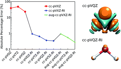
Standard quantum chemical basis sets are generally optimized to closely reproduce the behavior of atomic orbitals75 and results in unacceptable errors if used to decompose the electronic density (Fig. 1). In contrast, specialized basis sets used in the density fitting approximation (also known as resolution-of-the-identity (RI) approximation)76–82 are specifically optimized to represent a linear expansion of one-electron charge densities obtained from the product of atomic orbitals. Using the RI-auxiliary basis sets {ϕRIk}, the total electron density field can be expressed as:
 | (1) |
As shown in Fig. 1, the use of the RI-auxiliary basis sets results in nearly two orders of magnitude increase in the overall accuracy with respect to the corresponding standard basis set. The addition of diffuse functions marginally improves the performance of the decomposition, but leads to instabilities of the overlap matrix (high condition number) and increases dramatically the number of basis functions per atom.
In practice, Weigend's cc-pVQZ/JKFIT81 basis set (henceforth: cc-pVQZ-RI) offers the best trade-off between accuracy and computational demand and therefore represents the best choice for the density decomposition.
2.1 Computational details
The dataset of molecular dimers has been selected from the side-chain side-chain interaction (SSI) subset of the BioFragment database (BFDb).73 The original set is made of 3380 dimers formed by amino-acids side-chain fragments taken from 47 different protein structures. Dimers with more than 25 atoms as well as those containing sulfur atoms were not considered. While the total number of sulfur-containing structures is too small to enable the machine-learning model to accurately capture its rich chemistry, the inclusion of the larger systems does not increase dramatically the chemical diversity of the dataset. The final dataset contains a total of 2291 dimers.As shown in Fig. 2, the complete set of 2291 dimers spans a large variety of dominant interaction types, ranging from purely dispersion dominated complexes (in blue) to mixed-influence (green and yellow) to hydrogen-bonded and charged systems (red). We retain the same classification criteria as in the original database to attribute the nature of the dominant interaction.
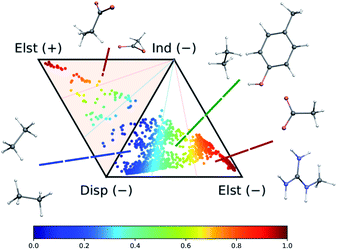 | ||
| Fig. 2 Ternary diagram representation of the attractive components of the dimer interaction energies for the 2291 systems considered in this work. The values of the SAPT analysis are taken from ref. 73. | ||
For each dimer, the reference full-electron density has been computed at the ωB97X-D/cc-pVQZ level using the resolution of identity approximation for the Coulomb and exchange potential (RI-JK). This implies that RI-auxiliary functions up to l = 5 are included for carbon, nitrogen and oxygen atoms while auxiliary functions up to l = 4 are used for hydrogen atoms.
3 Results and discussion
The training set for the density-learning model was chosen by randomly picking 2000 dimers out of a total of 2291 possibilities. The remaining 291 were used to test the accuracy of the predictions. Given the tremendous number of possible atomic environments (∼40![[thin space (1/6-em)]](https://www.rsc.org/images/entities/char_2009.gif) 000) associated with such a chemically diverse database, a subset of M reference environments was selected to reduce the dimensionality of the regression problem (see ESI†). To assess the consequences of this dimensionality reduction, the learning exercise was performed on three different sizes M = {100, 500, 1000} for the reference atomic environments. Fig. 3 summarizes the performance of the machine learning algorithm, expressed in terms of the mean absolute difference between the predicted and the reference densities (QM). Here, only the machine-learning error is shown as the reference densities derive from the RI-expansion of the computed ab initio densities. Since the test set contains molecules of different sizes, the contribution of each dimer has been weighted considering the ratio between its number of electrons and the total number of electrons in the test set.
000) associated with such a chemically diverse database, a subset of M reference environments was selected to reduce the dimensionality of the regression problem (see ESI†). To assess the consequences of this dimensionality reduction, the learning exercise was performed on three different sizes M = {100, 500, 1000} for the reference atomic environments. Fig. 3 summarizes the performance of the machine learning algorithm, expressed in terms of the mean absolute difference between the predicted and the reference densities (QM). Here, only the machine-learning error is shown as the reference densities derive from the RI-expansion of the computed ab initio densities. Since the test set contains molecules of different sizes, the contribution of each dimer has been weighted considering the ratio between its number of electrons and the total number of electrons in the test set. | (2) |
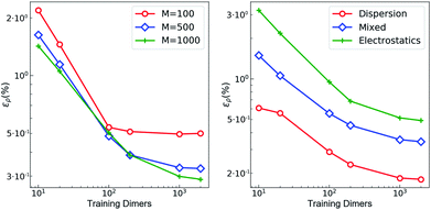 | ||
| Fig. 3 Learning curves with respect to RI-expanded densities (ML error). (left) weighted mean absolute percentage error (ερ (%)) of the predicted SA-GPR densities as a function of the number of training dimers. The weights correspond to the number of electrons in each dimer and the normalization is defined by the total number of electrons. Color code reflects the number of reference environments. (right) ερ (%) of the predicted SA-GPR densities (M = 1000) divided per dominant contribution to the interaction energy according to ref. 73. | ||
As shown in the first panel of Fig. 3, 100 training dimers were sufficient to reach saturation of the density error around 0.5% for M = 100. This result already outperforms the level of accuracy reached in our previous work, which is remarkable given the large chemical diversity of the dataset and the consideration of all-electron densities. Learning curves obtained with M = 500 and M = 1000 show steeper slopes, approaching saturation at about 2000 training dimers with errors that were reduced to ∼0.2–0.3%. The predicted full-electron densities are five times more accurate than the previous predictions of valence-only densities (approximately 1%).58 A more detailed analysis of the M = 1000 learning curve reveals a strong dependence on the nature of the dominant interaction (Fig. 3). Specifically, a stronger non-local character in the interaction yields a larger error. This is especially prevalent for dimers dominated by electrostatic interactions (i.e., hydrogen bonds, charged systems), which are characterized by errors that are twice as large as those found in other regimes.
The origin of this slow convergence arises from two factors. First, only about 20% of the dimers are dominantly bound by electrostatics.73 The priority of the regression model is thus to minimize the error on the other classes. Second, there is a fundamental dichotomy between the local nature of our symmetry-adapted learning scheme and the long-range nature of the interactions. In fact, the electron density encodes information about the whole chemical system at once, while the machine-learning model represents molecules as a collection of 4 Å wide atom-centered environments. This difference in the spatial reach of the information encoded in the target and in the representation is a limitation. In this respect, a global molecular representation, which includes the whole chemical system, would be more suitable, but this would imply renouncing to the scalability and transferability of the model. Given a large enough training set, however, our SA-GPR model is able to capture the density deformations due to the field generated by the neighboring molecule. The reason is rooted in the intrinsic locality of density deformations and in the concept of “nearsightedness”83,84 of all local electronic properties, which constitutes a theoretical justification for a local decomposition of such quantities.
The fundamental advantage of setting the electron density as the machine-learning target is the broad spectrum of chemical properties that are directly derivable from ρ(r). For instance, the predicted charge densities are the key ingredient in density-dependent scalar fields aimed at visualizing and characterizing interactions between atoms and molecules in real space. Examples of the density overlap region indicator (DORI)30 are given in Fig. 4 for representative dimers. Compared to the rather featureless ρ(r), DORI reveals fine details of the electronic structure, which constitute a more sensitive probe for the quality of the machine-learning predictions. In particular, it reveals density overlaps (or clashes) associated with bonding and non-covalent regions on equal footing through the behavior of the local wave-vector (∇ρ(r)/ρ(r)).85–87
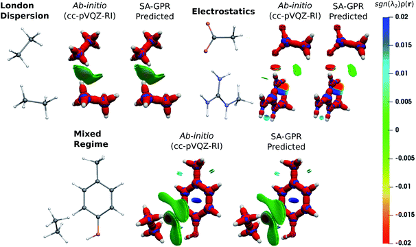 | ||
| Fig. 4 DORI maps of representative dimers for each type of dominant interaction (DORI isovalue: 0.9). Isosurfaces are color-coded31 with sgn(λ2)ρ(r) in the range from attractive −0.02 a.u. (red) to repulsive 0.02 a.u. (blue). In particular, sgn(λ2)ρ(r) < 0 characterizes covalent bonds or strongly attractive NCIs (e.g. H-bonds); sgn(λ2)ρ(r) ∼ 0 indicates weak attractive interactions (van der Waals); sgn(λ2)ρ(r) > 0 repulsive NCIs (e.g. steric clashes). | ||
As shown in Fig. 4, the intra- and intermolecular DORI domains obtained with the SA-GPR densities are indistinguishable from those in the ab initio maps. This performance is especially impressive for the density clashes associated with low-density values, as is typical for the non-covalent domains. All the features are well captured by the predicted densities ranging from large and delocalized basins typical of the van der Waals complexes (in green) to the compact and directional domains typical of electrostatic interactions to intramolecular steric clashes (e.g. phenol, mixed regime). A quantitative measure of the DORI accuracy for the most characteristic basin of each type of interaction is reported in the ESI.† Overall, these results illustrate that the residual 0.2% mean absolute percentage error does not significantly affect the density amplitude in the valence and intermolecular regions that are accurately described by the SA-GPR model. The highest amplitude errors are concentrated near the nuclei in the region dominated by the core-density fluctuations.
The versatility of the machine-learning prediction is further illustrated by using the predicted densities to compute the molecular electrostatic potential (ESP) for the same representative dimers (Fig. 5). ESP maps based on predicted densities agree quantitatively with the ab initio reference and correctly attribute the sign and magnitude of the electrostatic potential in all regions of space. Importantly, the accuracy of the ESP magnitude remains largely independent of the dominant interaction type. This is especially relevant for charged dimers (electrostatics) as it demonstrates that despite slower convergence of the learning curve for this category, the achieved accuracy of the model is sufficient to describe the key features of the electrostatic potential.
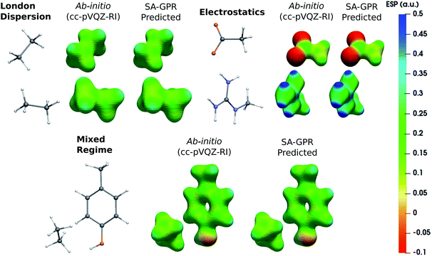 | ||
| Fig. 5 Electrostatic potential (ESP) maps of representative dimers for each type of dominant interaction (density isovalue: 0.05 e− bohr−3). ESP potential is given in Hartree atomic units (a.u.). | ||
The most widespread applications of ESP maps exploit qualitative information (e.g., identification of the molecular regions most prone to electrophilic/nucleophilic attack) but the electrostatic potentials can be related to quantitative properties such as the degree of acidity of hydrogen bonds and the magnitude of binding energies.88–92 As a concrete example related to structure-based drug design, we used a recent model that estimates the strength of the stacking interactions between heterocycles and aromatic amino acid side-chains directly from the ESP maps.88,91,93 This model derives the stacking energies of drug-like heterocycles from the maximum and mean value of their ESP within a surface delimited by molecular van der Waals volume (at 3.25 Å above the molecular plane).88 Following this procedure, we used the ESP derived from the ML predicted densities to compute the binding energies between a representative heterocycle included in our dataset, the tryptophan side-chain, and the three aromatic amino acid side-chains (Fig. 6).
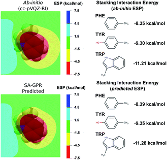 | ||
| Fig. 6 (left) Electrostatic potential maps 3.25 Å above the plane of the tryptophan (TRP) side-chain. The van der Waals volume of TRP is represented in transparency. The color code represents the electrostatic potential in kcal mol−1 according the scale chosen in ref. 88. (Right) Stacking interaction energies of TRP with the phenylalanine (PHE), tyrosin (TYR) and tryptophan (TRP) side-chains computed as detailed in ref. 88 on the basis of ab initio (top) and ML-predicted (bottom) ESP. | ||
Comparison between ab initio and ML predicted stacking interaction energies shows that the deviations in the ESP maps lead to minor errors on the order of 0.05 kcal mol−1. The largest deviations in the ESP would appear further away from the molecule, beyond the region exploited for the computation of the energy descriptors (i.e., the sum of the atomic van der Waals radii). The predicted ESP shows larger relative deviations far from the nuclei owing to the error propagation of the density predictions ρ(r) to the electrostatic potential ϕ(r). This can be best understood in the reciprocal space, where the deviations of the potential at a given wave-vector k are related to the density error by δ![[small phi, Greek, circumflex]](https://www.rsc.org/images/entities/i_char_e0b5.gif) (k) = 4πδ
(k) = 4πδ![[small rho, Greek, circumflex]](https://www.rsc.org/images/entities/i_char_e0b7.gif) (k)/k2. Because of the k−2 scaling, the error on ϕ(k) increases as k → 0, implying that larger relative errors of the electrostatic potential are expected in regions of space where ϕ(r) is slowly varying (i.e., thus determined by the long-wavelength components).
(k)/k2. Because of the k−2 scaling, the error on ϕ(k) increases as k → 0, implying that larger relative errors of the electrostatic potential are expected in regions of space where ϕ(r) is slowly varying (i.e., thus determined by the long-wavelength components).
3.1 Prediction on polypeptides
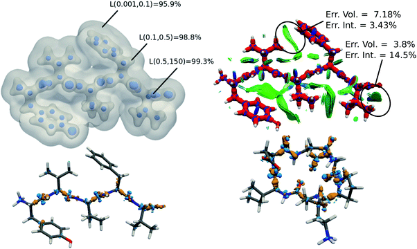
The tremendous advantage of the atom-centered density decomposition is to deliver a machine-learning model that depends only on the different atomic environments and not on the identity of the molecules included in the training set. Thanks to its transferability, the model provides access to density information of large macromolecules, at the sole price of including sufficient diversity, that can capture the chemical complexity of a larger system. The predictive power of this extrapolation procedure is demonstrated by using the machine-learning model exclusively trained on the 2291 BFDb dimers to predict the electron density of 8 polypeptides taken from the Protein DataBank (PDB).94 The performance of the ML model for each macromolecule, labeled by their PBD ID, is reported in Fig. 8.Overall, the predictions lead to a low average error of only 1.5% for the 8 polypeptides, which is in line with the highest density errors obtained on the BFDb test set. Relevantly, the largest discrepancies are obtained for 3WNE, which is the only cyclopeptide of the set. The origin of these differences can be understood by performing a more detailed analysis of a representative polypeptide, the leu-enkephalin (4OLR). The errors in this percentage range do not affect the density-based properties, such as the spatial analysis of the non-covalent interactions with scalar fields (Fig. 7 top right panel). Yet, the density differences indicate that the highest absolute errors occur along the amino acid backbone (Fig. 7 lower panels). In addition, the analysis of the relative error with the Walker–Mezey L(a,a′) index34 shows the highest similarity at the core (99.3%), slowly decreasing while approaching the non-covalent domain (96.3%) (Fig. 7 top left panel). The L(a,a′) index complements the density difference information by showing that the actual density amplitudes and the prediction error do not decrease at the same rate. Nevertheless, the loss of relative accuracy remains modest and the quality of the density is mainly governed by the predictions along the peptide backbone, which are especially sensitive for the more strained 3WNE cyclopeptide. Although similar chemical environments were included in the training set, the error is mainly determined by the lack of an explicit peptide bond motif and cyclopeptides in the training set. While this limitation could be addressed by ad hoc modification of the training set, the overall performance of the machine-learning model is rather exceptional as it provides in only a few minutes, instead of almost a day (about 500 times faster for e.g. enkephalin with the same functional and basis set), electron densities of DFT quality for large and complex molecular systems. For comparison, the superposition of atomic densities (i.e., the promolecular approach), which has been used to qualitatively analyze non-covalent interactions in peptides and proteins (e.g.ref. 32) lead to much larger mean absolute percentage errors (17 times higher, see Fig. S1 in the ESI†).
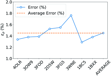 | ||
| Fig. 8 Weighted mean absolute percentage error (ερ (%)) with respect to ωB97X-D/cc-pVQZ densities of the predicted densities extrapolated for 8 biologically relevant peptides (protein databank ID). | ||
4 Conclusion
Given its central role in electronic structure methods, the total electron density is a very promising target for machine learning, since accurate predictions of ρ(r) give access to all the information needed to characterize a chemical system. Among the many possible properties that can be computed from the electron density, the patterns arising from non-covalent interactions constitute a particular challenge for machine learning models owing to their long-range nature and subtle physical origin. An effective ML model should be transferable across different systems, efficient in learning from relatively small training sets, and accurate in predicting ρ(r) both in the quickly-varying region around the atomic nuclei, in the tail and – crucially for the study of non-covalent interactions – in those regions that are characterized by low densities and low density gradients. In this work, we have presented a model that fulfills all of these requirements, based on an atom-centered decomposition of the density with a quadruple-zeta resolution-of-identity basis set, a symmetry-adapted Gaussian Process regression ML scheme, and training on a diverse database of 2000 sidechain–sidechain dimers extracted from the BioFragment database.The model reaches a 0.3% accuracy on a validation set, that is sufficient to investigate density-based fingerprints of NCIs, and to evaluate the electrostatic potential with sufficient accuracy to quantitatively estimate residue–residue interactions. The transferability of the model is demonstrated by predicting, at a cost that is orders of magnitude smaller than by explicit electronic structure calculations, the electron density for a demonstrative set of oligopeptides, with an accuracy sufficient to reliably visualize bonding patterns and non-covalent domains using the DORI scalar field. Even though the model reaches an impressive accuracy (0.5% mean absolute percentage error) for dimers that are predominantly bound by electrostatic interactions, the comparatively larger error suggests that future work should focus on resolving the dichotomy between the local machine learning framework and the long-range nature of the intermolecular interactions.
Conflicts of interest
There are no conflicts to declare.Acknowledgements
The National Centre of Competence in Research (NCCR) “Materials' Revolution: Computational Design and Discovery of Novel Materials (MARVEL)” of the Swiss National Science Foundation (SNSF) and the EPFL are acknowledged for financial support.Notes and references
- A. Stone, The Theory of Intermolecular Forces, Oxford University Press, 2013 Search PubMed.
- A. D. Buckingham, P. W. Fowler and J. M. Hutson, Chem. Rev., 1988, 88, 963–988 CrossRef CAS.
- A. Castleman Jr and P. Hobza, Chem. Rev., 1994, 94, 1721–1722 CrossRef.
- B. Brutschy and P. Hobza, Chem. Rev., 2000, 100, 3861–3862 CrossRef CAS PubMed.
- P. Hobza and J. Řezáč, Chem. Rev., 2016, 116, 4911–4912 CrossRef CAS PubMed.
- E. Pastorczak and C. Corminboeuf, J. Chem. Phys., 2017, 146, 120901 CrossRef PubMed.
- R. Parr and Y. Weitao, Density-Functional Theory of Atoms and Molecules, Oxford University Press, 1994 Search PubMed.
- W. Kohn and L. J. Sham, Phys. Rev., 1965, 140, A1133–A1138 CrossRef.
- A. J. Cohen, P. Mori-Sánchez and W. Yang, Chem. Rev., 2012, 112, 289–320 CrossRef CAS PubMed.
- A. D. Becke, J. Chem. Phys., 2014, 140, 18A301 CrossRef PubMed.
- N. Mardirossian and M. Head-Gordon, Mol. Phys., 2017, 115, 2315–2372 CrossRef CAS.
- D. Porezag and M. R. Pederson, Phys. Rev. B: Condens. Matter Mater. Phys., 1996, 54, 7830–7836 CrossRef CAS PubMed.
- M. K. Gilson and B. H. Honig, Nature, 1987, 330, 84–86 CrossRef CAS PubMed.
- S. Mecozzi, A. P. West and D. A. Dougherty, Proc. Natl. Acad. Sci. U. S. A., 1996, 93, 10566–10571 CrossRef CAS PubMed.
- T. Sagara, J. Klassen and E. Ganz, J. Chem. Phys., 2004, 121, 12543 CrossRef CAS PubMed.
- S. Cardamone, T. J. Hughes and P. L. A. Popelier, Phys. Chem. Chem. Phys., 2014, 16, 10367 RSC.
- P. L. Polavarapu, J. Phys. Chem., 1990, 94, 8106–8112 CrossRef CAS.
- J. L. P. Hughes and J. E. Sipe, Phys. Rev. B: Condens. Matter Mater. Phys., 1996, 53, 10751–10763 CrossRef CAS PubMed.
- J. E. Sipe and A. I. Shkrebtii, Phys. Rev. B: Condens. Matter Mater. Phys., 2000, 61, 5337–5352 CrossRef CAS.
- S. Sharma and C. Ambrosch-Draxl, Phys. Scr., T, 2004, 109, 128 CrossRef.
- A. E. Masunov, A. Tannu, A. A. Dyakov, A. D. Matveeva, A. Y. Freidzon, A. V. Odinokov and A. A. Bagaturyants, J. Chem. Phys., 2017, 146, 244104 CrossRef PubMed.
- T. S. Koritsanszky and P. Coppens, Chem. Rev., 2001, 101, 1583–1628 CrossRef CAS PubMed.
- C. Lecomte, B. Guillot, N. Muzet, V. Pichon-Pesme and C. Jelsch, Cell. Mol. Life Sci., 2004, 61, 774–782 CrossRef CAS PubMed.
- D. Jayatilaka and B. Dittrich, Acta Crystallogr., Sect. A: Found. Crystallogr., 2008, 64, 383–393 CrossRef CAS PubMed.
- M. J. Schnieders, T. D. Fenn, V. S. Pande and A. T. Brunger, Acta Crystallogr., Sect. D: Biol. Crystallogr., 2009, 65, 952–965 CrossRef CAS PubMed.
- A. Brunger and P. Adams, Comprehensive Biophysics, Elsevier, 2012, pp. 105–115 Search PubMed.
- C. Gatti and P. Macchi, Modern Charge-Density Analysis, Springer Netherlands, Dordrecht, 2012 Search PubMed.
- R. F. W. Bader, Chem. Rev., 1991, 91, 893–928 CrossRef CAS.
- R. Bader, The Quantum Theory of Atoms in Molecules, Wiley-VCH Verlag GmbH & Co. KGaA, Weinheim, Germany, 2007 Search PubMed.
- P. de Silva and C. Corminboeuf, J. Chem. Theory Comput., 2014, 10, 3745–3756 CrossRef CAS PubMed.
- E. R. Johnson, S. Keinan, P. Mori-Sánchez, J. Contreras-García, A. J. Cohen and W. Yang, J. Am. Chem. Soc., 2010, 132, 6498–6506 CrossRef CAS PubMed.
- J. Contreras-García, E. R. Johnson, S. Keinan, R. Chaudret, J.-P. Piquemal, D. N. Beratan and W. Yang, J. Chem. Theory Comput., 2011, 7, 625–632 CrossRef PubMed.
- P. D. Walker and P. G. Mezey, J. Am. Ceram. Soc., 1993, 115, 12423–12430 CAS.
- P. D. Walker and P. G. Mezey, J. Am. Chem. Soc., 1994, 116, 12022–12032 CrossRef CAS.
- T. E. Exner and P. G. Mezey, J. Phys. Chem. A, 2002, 106, 11791–11800 CrossRef CAS.
- T. E. Exner and P. G. Mezey, J. Comput. Chem., 2003, 24, 1980–1986 CrossRef CAS.
- Z. Szekeres, T. Exner and P. G. Mezey, Int. J. Quantum Chem., 2005, 104, 847–860 CrossRef CAS.
- H. Stoll, G. Wagenblast and H. Preuβ, Theor. Chim. Acta, 1980, 57, 169–178 CrossRef CAS.
- B. Meyer, B. Guillot, M. F. Ruiz-Lopez and A. Genoni, J. Chem. Theory Comput., 2016, 12, 1052–1067 CrossRef CAS PubMed.
- B. Meyer, B. Guillot, M. F. Ruiz-Lopez, C. Jelsch and A. Genoni, J. Chem. Theory Comput., 2016, 12, 1068–1081 CrossRef CAS PubMed.
- B. Meyer and A. Genoni, J. Phys. Chem. A, 2018, 122, 8965–8981 CrossRef CAS PubMed.
- F. L. Hirshfeld, Acta Crystallogr., Sect. B: Struct. Crystallogr. Cryst. Chem., 1971, 27, 769–781 CrossRef CAS.
- R. F. Stewart, Acta Crystallogr., Sect. A: Found. Crystallogr., 1976, 32, 565–574 CrossRef.
- N. K. Hansen and P. Coppens, Acta Crystallogr., Sect. A: Found. Crystallogr., 1978, 34, 909–921 CrossRef.
- V. Pichon-Pesme, C. Lecomte and H. Lachekar, J. Phys. Chem., 1995, 99, 6242–6250 CrossRef CAS.
- C. Jelsch, V. Pichon-Pesme, C. Lecomte and A. Aubry, Acta Crystallogr., Sect. D: Biol. Crystallogr., 1998, 54, 1306–1318 CrossRef CAS PubMed.
- B. Zarychta, V. Pichon-Pesme, B. Guillot, C. Lecomte and C. Jelsch, Acta Crystallogr., Sect. A: Found. Crystallogr., 2007, 63, 108–125 CrossRef CAS PubMed.
- C. Lecomte, C. Jelsch, B. Guillot, B. Fournier and A. Lagoutte, J. Synchrotron Radiat., 2008, 15, 202–203 CrossRef CAS PubMed.
- S. Domagala, P. Munshi, M. Ahmed, B. Guillot and C. Jelsch, Acta Crystallogr., Sect. B: Struct. Crystallogr. Cryst. Chem., 2011, 67, 63–78 CrossRef CAS.
- S. Domagala, B. Fournier, D. Liebschner, B. Guillot and C. Jelsch, Acta Crystallogr., Sect. A: Found. Crystallogr., 2012, 68, 337–351 CrossRef CAS PubMed.
- T. Koritsanszky, A. Volkov and P. Coppens, Acta Crystallogr., Sect. A: Found. Crystallogr., 2002, 58, 464–472 CrossRef.
- P. M. Dominiak, A. Volkov, X. Li, M. Messerschmidt and P. Coppens, J. Chem. Theory Comput., 2007, 3, 232–247 CrossRef CAS.
- B. Dittrich, T. Koritsánszky and P. Luger, Angew. Chem., Int. Ed., 2004, 43, 2718–2721 CrossRef CAS.
- V. R. Hathwar, T. S. Thakur, T. N. G. Row and G. R. Desiraju, Cryst. Growth Des., 2011, 11, 616–623 CrossRef CAS.
- F. Brockherde, L. Vogt, L. Li, M. E. Tuckerman, K. Burke and K.-R. Müller, Nat. Commun., 2017, 8, 872 CrossRef PubMed.
- M. Bogojeski, F. Brockherde, L. Vogt-Maranto, L. Li, M. E. Tuckerman, K. Burke and K.-R. Müller, arXiv:1811.06255, 2018.
- A. Grisafi, D. M. Wilkins, G. Csányi and M. Ceriotti, Phys. Rev. Lett., 2018, 120, 036002 CrossRef CAS.
- A. Grisafi, A. Fabrizio, B. Meyer, D. M. Wilkins, C. Corminboeuf and M. Ceriotti, ACS Cent. Sci., 2019, 5, 57–64 CrossRef CAS.
- J. M. Alred, K. V. Bets, Y. Xie and B. I. Yakobson, Compos. Sci. Technol., 2018, 166, 3–9 CrossRef CAS.
- A. Chandrasekaran, D. Kamal, R. Batra, C. Kim, L. Chen and R. Ramprasad, npj Comput. Mater., 2019, 5, 22 CrossRef.
- A. T. Fowler, C. J. Pickard and J. A. Elliott, Journal of Physics: Materials, 2019, 2, 034001 Search PubMed.
- P. Jurečka, J. Šponer, J. Černý and P. Hobza, Phys. Chem. Chem. Phys., 2006, 8, 1985–1993 RSC.
- Y. Zhao and D. G. Truhlar, Acc. Chem. Res., 2008, 41, 157–167 CrossRef CAS PubMed.
- J. Řezáč, K. E. Riley and P. Hobza, J. Chem. Theory Comput., 2011, 7, 2427–2438 CrossRef PubMed.
- L. A. Burns, Á. Vázquez-Mayagoitia, B. G. Sumpter and C. D. Sherrill, J. Chem. Phys., 2011, 134, 084107 CrossRef PubMed.
- M. S. Marshall, L. A. Burns and C. D. Sherrill, J. Chem. Phys., 2011, 135, 194102 CrossRef PubMed.
- D. G. A. Smith, L. A. Burns, K. Patkowski and C. D. Sherrill, J. Phys. Chem. Lett., 2016, 7, 2197–2203 CrossRef CAS.
- S. Grimme, Chem.–Eur. J., 2012, 18, 9955–9964 CrossRef CAS PubMed.
- T. Risthaus and S. Grimme, J. Chem. Theory Comput., 2013, 9, 1580–1591 CrossRef CAS PubMed.
- S. T. Schneebeli, A. D. Bochevarov and R. A. Friesner, J. Chem. Theory Comput., 2011, 7, 658–668 CrossRef CAS.
- N. Mardirossian and M. Head-Gordon, J. Chem. Phys., 2016, 144, 214110 CrossRef PubMed.
- R. T. McGibbon, A. G. Taube, A. G. Donchev, K. Siva, F. Hernández, C. Hargus, K.-H. Law, J. L. Klepeis and D. E. Shaw, J. Chem. Phys., 2017, 147, 161725 CrossRef PubMed.
- L. A. Burns, J. C. Faver, Z. Zheng, M. S. Marshall, D. G. Smith, K. Vanommeslaeghe, A. D. MacKerell, K. M. Merz and C. D. Sherrill, J. Chem. Phys., 2017, 147, 161727 CrossRef PubMed.
- A. Grisafi, D. M. Wilkins, M. J. Willatt and M. Ceriotti, arXiv:1904.01623, 2019.
- T. Helgaker, P. Jørgensen and J. Olsen, Molecular Electronic-Structure Theory, John Wiley & Sons, Ltd, Chichester, UK, 2000 Search PubMed.
- J. L. Whitten, J. Chem. Phys., 1973, 58, 4496–4501 CrossRef CAS.
- B. I. Dunlap, J. W. D. Connolly and J. R. Sabin, Int. J. Quantum Chem., Symp., 1977, 11, 81–87 CrossRef CAS.
- M. Feyereisen, G. Fitzgerald and A. Komornicki, Chem. Phys. Lett., 1993, 208, 359–363 CrossRef CAS.
- A. P. Rendell and T. J. Lee, J. Chem. Phys., 1994, 101, 400–408 CrossRef CAS.
- K. Eichkorn, O. Treutler, H. Öhm, M. Häser and R. Ahlrichs, Chem. Phys. Lett., 1995, 240, 283–290 CrossRef CAS.
- F. Weigend, Phys. Chem. Chem. Phys., 2002, 4, 4285–4291 RSC.
- H.-J. Werner, F. R. Manby and P. J. Knowles, J. Chem. Phys., 2003, 118, 8149–8160 CrossRef CAS.
- W. Kohn, Phys. Rev. Lett., 1996, 76, 3168–3171 CrossRef CAS PubMed.
- E. Prodan and W. Kohn, Proc. Natl. Acad. Sci. U. S. A., 2005, 102, 11635–11638 CrossRef CAS PubMed.
- A. Nagy and N. H. March, Mol. Phys., 1997, 90, 271–276 CrossRef CAS.
- H. J. Bohórquez and R. J. Boyd, J. Chem. Phys., 2008, 129, 024110 CrossRef PubMed.
- Á. Nagy and S. Liu, Phys. Lett. A, 2008, 372, 1654–1656 CrossRef.
- A. N. Bootsma, A. C. Doney and S. Wheeler, chemrxiv.7628939.v4, 2019.
- J. S. Murray, T. Brinck, P. Lane, K. Paulsen and P. Politzer, J. Mol. Struct., 1994, 307, 55–64 CrossRef.
- J. S. Murray and P. Politzer, J. Mol. Struct., 1998, 425, 107–114 CrossRef CAS.
- A. N. Bootsma and S. Wheeler, chemrxiv.8079890.v1, 2019.
- A. Volkov, T. Koritsanszky and P. Coppens, Chem. Phys. Lett., 2004, 391, 170–175 CrossRef CAS.
- A. N. Bootsma and S. E. Wheeler, J. Chem. Inf. Model., 2019, 59, 149–158 CrossRef CAS PubMed.
- H. M. Berman, Nucleic Acids Res., 2000, 28, 235–242 CrossRef CAS PubMed.
Footnote |
| † Electronic supplementary information (ESI) available. See DOI: 10.1039/c9sc02696g |
| This journal is © The Royal Society of Chemistry 2019 |

