MGraphDTA: deep multiscale graph neural network for explainable drug–target binding affinity prediction

Abstract

Predicting drug–target affinity (DTA) is beneficial for accelerating drug discovery. Graph neural networks (GNNs) have been widely used in DTA prediction. However, existing shallow GNNs are insufficient to capture the global structure of compounds. Besides, the interpretability of the graph-based DTA models highly relies on the graph attention mechanism, which can not reveal the global relationship between each atom of a molecule. In this study, we proposed a deep multiscale graph neural network based on chemical intuition for DTA prediction (MGraphDTA). We introduced a dense connection into the GNN and built a super-deep GNN with 27 graph convolutional layers to capture the local and global structure of the compound simultaneously. We also developed a novel visual explanation method, gradient-weighted affinity activation mapping (Grad-AAM), to analyze a deep learning model from the chemical perspective. We evaluated our approach using seven benchmark datasets and compared the proposed method to the state-of-the-art deep learning (DL) models. MGraphDTA outperforms other DL-based approaches significantly on various datasets. Moreover, we show that Grad-AAM creates explanations that are consistent with pharmacologists, which may help us gain chemical insights directly from data beyond human perception. These advantages demonstrate that the proposed method improves the generalization and interpretation capability of DTA prediction modeling.

---

1 Introduction

Drug discovery aims to detect drugs that can bind to the target and then change disease progression. The identification of drug–target interactions is an important step in developing new drugs and understanding their side effects.¹ Binding affinity provides information on the strength of the interaction between a drug–target pair, and it is usually expressed in measures such as dissociation constant (K_d), inhibition constant (K_i), or the half-maximal inhibitory concentration (IC₅₀).² Protein microarrays³ and affinity chromatography⁴ are two biological experimental methods to measure binding affinity. To identify effective and safe drugs for a given protein, pharmacologists have to test thousands of chemical compounds.⁵ However, the experimental measurement of drug–target affinities (DTAs) is both time- and resource-consuming. In silico methods for DTA prediction have received great attention due to their efficiency and low cost. The existing in silico methods can be mainly divided into three categories: structure-based methods, feature-based methods, and deep learning methods.

Structure-based methods can explore the potential binding sites by considering the 3D structure of a small molecule and a protein. Docking is a well-established structure-based method that uses numerous mode definitions and scoring functions to minimize free energy for binding. Molecular dynamics simulation is another popular structure-based method that can provide the ultimate detail concerning individual particle motions as a function of time.⁶ However, the structure-based methods are time-consuming and can not be employed if the 3D structure of the protein is unknown.⁷

Feature-based methods for DTA prediction modeling are also known as proteochemometrics (PCM),^8–10 which relies on a combination of explicit ligand and protein descriptors. Any pairs of drugs and targets can be represented in terms of biological feature vectors with a certain length, often with binary labels that determine whether the drug can bind to the target or not. The extracted biological feature vectors can be used to train machine/deep learning models such as feed-forward neural networks (FNNs), support vector machine (SVM), random forest (RF), and other kernel-based methods.^11–19 For example, DeepDTIs²⁰ chose the most common and simple features: extended connectivity fingerprints (ECFP) and protein sequence composition descriptors (PSC) for drugs and targets representation, and then used a deep belief network for DTA prediction. Lenselink et al.¹¹ compared FNNs with different machine learning methods such as logistic regression, RF, and SVM on one single standardized dataset and found that FNNs are the top-performing classifiers. A study conducted by Mayr et al.¹² also found a similar result that FNNs outperform other competing methods. MDeePred²¹ represented protein descriptors by the combination of various types of protein features such as sequence, structural, evolutionary, and physicochemical properties, and a hybrid deep neural network was used to predict binding affinities from the compound and protein descriptors. MoleculeNet²² introduced a featurization method called grid featurizer that used structural information of both ligand and target. The grid featurizer considers not only features of the protein and ligand individually but also the chemical interaction within the binding pocket.

Over the past few years, there has been a remarkable increase in the amount of available compound activity and biomedical data owing to the emergence of novel experimental techniques such as high throughput screening, parallel synthesis among others.^23–25 The high demand for exploring and analyzing massive data has encouraged the development of data-hungry algorithms like deep learning.^26,27 Many types of deep learning frameworks have been adopted in DTA prediction. DeepDTA² established two convolutional neural networks (CNNs) to learn the representations of the drug and protein, respectively. The learned drug and protein representations are then concatenating and fed into a multi-layer perceptron (MLP) for DTA prediction. WideDTA²⁸ further improved the performance of DeepDTA by integrating two additional text-based inputs and using four CNNs to encode them into four representations. Lee et al.²⁹ also utilized CNN on the protein sequence to learn local residue patterns and conduct extensive experiments to demonstrate the effectiveness of CNN-based methods. On the other hand, DEEPScreen represented compounds as 2-D structural images and used CNN to learn complex features from these 2-D structural drawings to produce highly accurate DTA predictions.³⁰

Although CNN-based methods have achieved remarkable performance in DTA prediction, most of these models represent the drugs as strings, which is not a natural way to represent compounds.³¹ When using strings, the structural information of the molecule is lost, which could impair the predictive power of a model as well as the functional relevance of the learned latent space. To address this problem, graph neural networks (GNNs) have been adopted in DTA prediction.^31–36 The GNN-based methods represent the drugs as graphs and use GNN for DTA prediction. For instance, Tsubaki et al.³⁴ proposed to use GNN and CNN to learn low-dimensional vector representation of compound graphs and protein sequences, respectively. They formulated the DTA prediction as a classification problem and conducted experiments on three datasets. The experimental results demonstrate that the GNN-based method outperforms PCM methods. GraphDTA³¹ evaluated several types of GNNs including GCN, GAT, GIN, and GAT–GCN for DTA prediction, in which DTA was regarded as a regression problem. The experimental results confirm that deep learning methods are capable of DTA prediction, and representing drugs as graphs can lead to further improvement. DGraphDTA³⁷ represented both compounds and proteins as graphs and used GNNs on both the compound and protein sides to obtain their representations. Moreover, to increase the model interpretability, attention mechanisms have been introduced into DTA prediction models.^{32,36,38–40}

On the other hand, some researches focused on improving DTA prediction by using structural-related features of protein as input.^37,41 For example, DGraphDTA³⁷ utilized contact maps predicted from protein sequences as the input of the protein encoder to improve the performance of DTA predictions. Since protein structural information is not always available, they use contact maps predicted from the sequences, which enables the model to take all sorts of proteins as input.

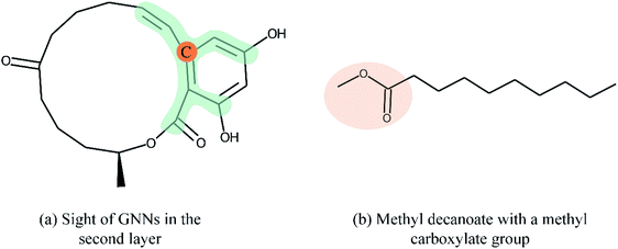
Overall, many novel models for DTA prediction based on shallow GNNs have been developed and show promising performance on various datasets. However, at least three problems have not been well addressed for GNN-based methods in DTA prediction. First, we argue that GNNs with few layers are insufficient to capture the global structure of the compounds. As shown in Fig. 1(a), a GNN with two layers is unable to know whether the ring exists in the molecule, and the graph embedding will be generated without considering the information about the ring. The graph convolutional layers should be stacked deeply in order to capture the global structure of a graph. Concretely, to capture the structures make up of k-hop neighbors, k graph convolutional layers should be stacked.⁴² However, building a deep architecture of GNNs is currently infeasible due to the over-smoothing and vanishing gradient problems.^43,44 As a result, most state-of-the-art (SOTA) GNN models are no deeper than 3 or 4 layers. Second, a well-constructed GNN should be able to preserve the local structure of a compound. As shown in Fig. 1(b), the methyl carboxylate moiety is crucial for methyl decanoate and the GNN should distinguish it from the less essential substituents in order to make a reasonable inference. Third, the interpretability of graph-based DTA models highly relies on the attention mechanism. Although the attention mechanism provides an effective visual explanation, it increases the computational cost. In addition, the graph attention mechanism only considers the neighborhood of a vertex (also called masked attention),^45,46 which can not capture the global relationship between each atom of a molecule.

Fig. 1 Both global and local structure information is important for GNN. (a) The sight of GNNs in the second layer is shown in green as we take the carbon with orange as the center. In this example, a GNN with two layers fails to identify the ring structure of zearalenone. (b) The GNN should preserve local structure information in order to distinguish the methyl carboxylate moiety (orange ellipse) from other less essential substituents.

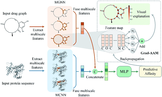
To address the above problems, we proposed a multiscale graph neural network (MGNN) and a novel visual explanation method called gradient-weighted affinity activation mapping (Grad-AAM) for DTA prediction and interpretation. An overview of the proposed MGraphDTA is shown in Fig. 2. The MGNN with 27 graph convolutional layers and a multiscale convolutional neural network (MCNN) were used to extract the multiscale features of drug and target, respectively. The multiscale features of the drug contained rich information about the molecule's structure at a different scale and enabled the GNN to make a more accurate prediction. The extracted multiscale features of the drug and target were fused respectively and then concatenated to obtain a combined descriptor for a given drug–target pair. The combined descriptor was fed into a MLP to predict binding affinity. Grad-AAM used the gradients of the affinity flowing into the final graph convolutional layer of MGNN to produce a probability map highlighting the important atoms that contribute most to the DTA. The proposed Grad-AAM was motivated by gradient-weighted class activation mapping (Grad-CAM) that can produce a coarse localization map highlighting the important regions in the image.⁴⁷ However, the Grad-CAM was designed for neural network classification tasks based CNNs. Unlike Grad-CAM, Grad-AAM was activated by the binding affinity score based on GNNs. The main contributions of this paper are twofold:

Fig. 2 Overview of the proposed MGraphDTA. The MGNN and MCNN were used to extract multiscale features of the input drug graph and protein sequence, respectively. The output multiscale features of the two encoders were fused respectively and then concatenated to obtain a combined representation of the drug–target pair. Finally, the combined representation was fed into a MLP to predict binding affinity. The Grad-AAM uses the gradient information flowing into the last graph convolutional layer of MGNN to understand the importance of each neuron for a decision of affinity.

(a) We construct a very deep GNN for DTA prediction and rationalize it from the chemical perspective.

(b) We proposed a simple but effective visualization method called Grad-AAM to investigate how GNN makes decisions in DTA prediction.

2 Methods

2.1 Input representation

The input molecules are SMILES (Simplified Molecular Input Line Entry System) that describes the structure of chemical species using short ASCII strings, while the input targets are protein sequences (strings) in which each character represents an amino acid. We preprocessed the SMILES into graphs with vertex (or node) features and adjacency matrix using RDkit⁴⁸ as shown in Fig. 3(a). More detailed information about the vertex features can be found in ESI Tables S1 and S2.† For protein sequences, we first built a vocabulary to map each character to an integer (e.g. alanine (A) is 1, cysteine (C) is 2, glutamic acid (E) is 4, and so on) so that the protein can be represented as an integer sequence. To make it convenient for training, we decided on fixed maximum lengths of 1200 for protein sequence so that the maximum lengths cover at least 80% of the proteins as suggested by the earlier study.² We then mapped each integer into a learnable 128-dimensional vector by an embedding layer^2,29 (i.e., each amino acid can be represented by a 128-dimensional embedding vector). Although one-hot vectors can also be used to encode proteins, they are not able to describe the semantical similarity between two different amino acids. For example, each pair of different one-hot vectors has a zero cosine similarity.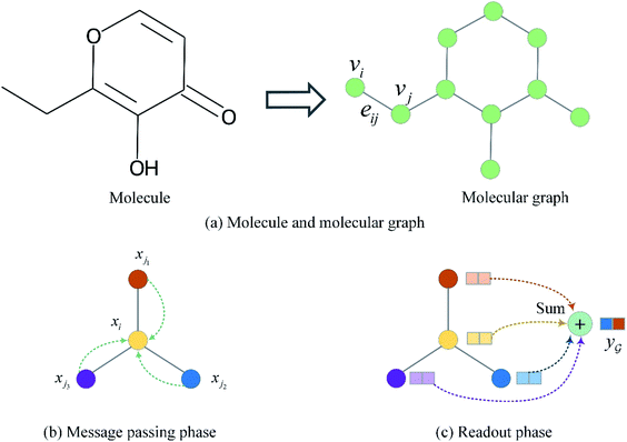

Fig. 3 Molecule representation and graph embedding. (a) Representing a molecule as a graph. (b) Graph message passing phase corresponding eqn (1). (c) Graph readout phase corresponding eqn (2).

2.2 Graph neural network

A graph is represented as where is the set of vertices and is the set of edges. In a molecule, is the i-th atom and is the chemical bond between i-th and j-th atoms. A GNN maps a graph to a vector usually with a message passing phase and readout phase.⁴⁹ As shown in Fig. 3(b) and (c), The message passing phase updates each vertex information by considering its neighboring vertices in , and the readout phase computes a feature vector y for the whole graph.

2.2.1 Message passing phase. Given a graph , we denoted the i-th vertex embedding at time step t as . We then updated x_i^(t) into using the following graph convolutional layer:⁵⁰where are learnable weight matrices shared across all vertices, is the set of neighbors of vertex i, and σ contains a node-level batch normalization⁴⁴ followed by a ReLU activation function, in which batch normalization is essential for very deep models.⁵¹ By using eqn (1) to aggregate the neighboring messages and iterate them over time steps, vertex embeddings can gradually gather more global information on the graph.

2.2.2 Readout phase. To obtain the final output vector y from the set of vertex vectors in , we take the average of the vertex embeddings:where is the number of vertices in the molecular graph, and L is the final time step. The readout phase aggregates vertex embeddings into a unified graph embedding.

2.3 Multiscale graph neural network for drug encoding

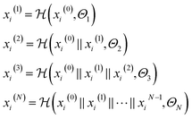
After representing the drug compounds as graphs, we designed a MGNN based on chemical intuition that learns effectively from graphical data. Fig. 4 shows the network architecture of the proposed MGNN. The MGNN includes three multiscale blocks in which each multiscale block is followed by a transition layer as shown in Fig. 4(a).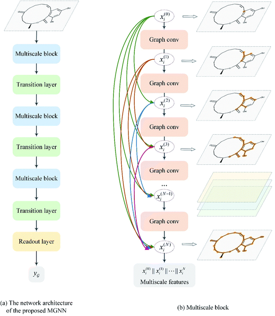

Fig. 4 Overview of the MGNN. (a) The network architecture of the proposed MGNN. (b) The detailed design of the multiscale block.

2.3.1 Multiscale block. A multiscale block contains N graph convolutional layers described by eqn (1). Motivated by DenseNet,^43,52 we introduced the dense connection into the GNN. The dense connection links each layer to every other layer in a feed-forward fashion, as shown in Fig. 4(b). Dense connections allow all layers to have direct access to receive the gradients of the loss function with respect to each weight, thereby avoiding the vanishing gradient problem and allowing for training very deep GNNs. Formally, we can express the multiscale block aswhere is a graph convolutional layer described by eqn (1) with parameters Θ_n (consist of W₁ and W₂) in which n represents n-th layer, and ∥ is the concatenate operation. The multiscale block extracts multiscale features which described the structure information of a molecule in both local and global contexts.

2.3.2 Transition layer. To increase the depth of the MGNN, we used the transition layers to connect two adjacent multiscale blocks. The transition layer aims to integrate the multiscale features from the previous multiscale block and reduce the channel number of the feature map. Specifically, for an input multiscale features at time step N + 1 as we expressed the transition layer as follow:where are learnable weight matrices shared across all vertices in which M = d + (N − 1)h. By using the transition layer, we reduced the channel numbers to half of the input to save computational cost. Finally, a readout layer described by eqn (2) was used to convert the whole graph to a feature vector

2.4 Multiscale convolutional neural network for target encoding

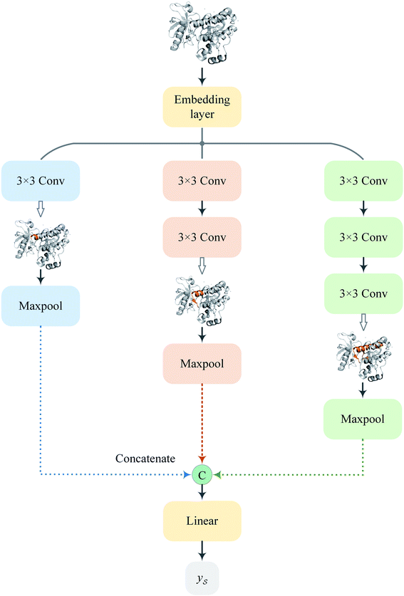
Following the idea of MGNN, we used a MCNN to extract the multiscale features of a protein, as shown in Fig. 5. In particular, we designed a network with three branches consisting of convolutional layers with different receptive fields to detect the local residue patterns of proteins at different scales. We increased the receptive fields by stacking 3 × 3 convolutional layers and the receptive fields of the three branches were 3, 5, and 7, respectively. Since there are only certain parts of a protein, such as specific domains or motifs, are involved in DTAs, rather than the whole protein structure.²⁹ As a result, increasing the receptive field to cover the whole protein sequence does not seem to be appropriate for DTA prediction due to noise information from the portions of the sequence that are not involved in DTA.²⁹ Formally, for an input integer protein sequence with a length of 1200, we first used an embedding layer^2,28,29,31 to map each integer to a 128-dimensional vector following the previous studies^2,28,31 and obtained an input matrix We then used the MCNN to map the S into a feature vector aswhere is the i-th branch with i 3 × 3 convolutional layers that maps into a matrix in which each convolutional layer is followed by ReLU activation, m represents maxpool operation that maps into a h-dimensional vector, and is a learnable matrix.

Fig. 5 The network architecture of the proposed MCNN.

2.5 MGraphDTA network architecture

After obtaining the vector representation of drug and target, the two representations are then concatenated and fed into a MLP to predict the binding affinity score, as shown in Fig. 2. Concretely, the MLP contains three linear transformation layers to map the combined representation into affinity score in which each linear transformation layer is followed by a ReLU activation and dropout layer with a dropout rate of 0.1 following with the previous studies.^2,28 MGraphDTA contains a MGNN for drug encoding, a MCNN for target encoding, and a MLP for DTA prediction, as shown in Fig. 2. We used the mean squared error (MSE) as the loss function as follows.where P_i and Y_i are the predictive score and the ground truth score of i-th drug–target pair, and n is the sample size. We also considered DTA prediction as a binary classification problem by simply replacing the MSE loss with cross-entropy loss.⁵³

2.6 Gradient-weighted affinity activation mapping

To improve the interpretation capability of DTA modeling, we proposed an attention-free visual interpretation method called Grad-AAM. Grad-AAM used the gradient information flowing into the last graph convolutional layer of the MGNN to understand the importance of each neuron for a decision of affinity. The graph convolutional layer naturally retains spatial information which is lost in fully connected layers. Therefore, we can expect the last graph convolutional layer to have the best compromise between high-level semantics and detailed spatial information.⁴⁷ Specifically, denoting the feature map of the last graph convolutional layer as A, in order to obtain the chemical probability map with vertex numbers for a given molecule, we first computed the gradient of the affinity score P with respect to a neuron A_v^k at k-th channel and v-th vertex of A as . Then the channel importance weights α_k can be computed as

We then performed a weighted combination of the forward activation maps followed by a ReLU activation as

Finally, min–max normalization was used to map the probability map P_Grad-AAM ranging from 0 to 1. The chemical probability map P_Grad-AAM can be thought of as a weighted aggregation of important geometric substructures of a molecule that are captured by a GNN as shown in Fig. 6.

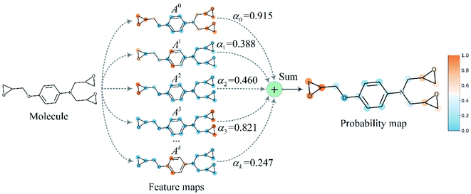Fig. 6 The chemical probability map is a weighted sum of vital substructures of a molecule captured by a GNN.

2.7 Dataset

The benchmark datasets for the regression task used in this study are the Metz,⁵⁴ KIBA,⁵⁵ Davis⁵⁶ datasets. The binding affinities of the three datasets are measured in inhibition constant (K_i), KIBA score,⁵⁵ and dissociation constant (K_d), respectively. Note that the Davis dataset is highly biased in terms of that all drug–target pairs where the activity could not be experimentally measured are labeled with 10 μM bioactivity value (i.e., pK_d value 5), and the number of data points that fit into this definition is extremely high (as shown in Fig. S1†). Therefore, we also evaluated the model's performance in the filtered Davis dataset²¹ in which data points with 10 μM bioactivity are removed.

We also formulated DTA prediction as a binary classification problem and evaluated the proposed MGraphDTA in two widely used classification datasets, Human and Caenorhabditis elegans (C. elegans).^34,38,46

Moreover, we conducted a case study to evaluate the Grad-AAM using the ToxCast dataset.³⁵ Since the ToxCast dataset contains multiple assays which means that one drug–target pair may have different binding affinity depending on the type of assay. For simplicity, we only selected one of the assays containing the largest drug–target pairs. Table 1 summarizes these datasets. Fig. S1–S3† show the distribution of binding affinities, SMILES length, and protein sequence length of these datasets.

Table 1 Summary of the seven datasets

Dataset	Task type	Compounds	Proteins	Interactions
Davis	Regression	68	442	30056
Filtered davis	Regression	68	379	9125
KIBA	Regression	2111	229	118254
Metz	Regression	1423	170	35259
Human	Classification	2726	2001	6728
C. elegans	Classification	1767	1876	7786
ToxCast	Regression	3098	37	114626

---

2.8 Experimental setup

Experiments were conducted using an NVIDIA GeForce GTX 2080TI with 11 GB memory. Adam optimizer⁵⁷ with a 0.0005 learning rate was used to update model parameters. The batch size was set to 512. We optimized the hyper-parameters for MGraphDTA in the training set of Davis under the five-fold cross-validation using an automatic hyper-parameters optimization software Optuna.⁵⁸ The optimized hyper-parameters were then kept fixed for all other datasets. Table S3† lists the detailed hyper-parameters setting. The MGNN consisted of 27 graph convolutional layers containing three multiscale blocks with N = 8 graph convolutional layers and three transition layers.

3 Results and discussion

3.1 Compare with SOTA DTA prediction models in classification tasks

For the classification task, we used the area under curve (AUC), precision, and recall as performance metrics to evaluate the model following the previous studies.^34,38,46 We compared the MGraphDTA with the SOTA GNN,³⁴ GraphDTA,³¹ TrimNet,⁴⁶ VQA-seq,⁴¹ and TransformerCPI³⁸ models. It should be noted that DrugVQA⁴¹ uses structural-related features of protein as input, while its alternative version VQA-seq⁴¹ that only uses protein sequence information is listed here for a fair comparison. To ensure a fair comparison, we experimented with the same dataset and data split scheme as the previous studies.^34,46 GraphDTA³¹ was originally designed for regression tasks and had been tailored for classification tasks by Chen et al.³⁸ and we used the results they reported for comparisons. All experiments were repeated three times, each with a different random seed following the previous studies.^38,41 We finally reported the mean and standard deviation of results in DTA prediction.

Table 2 summarizes the quantitative results. For the Human dataset, the proposed method yielded a significantly higher precision than that of other methods for DTA prediction. For the C. elegans dataset, the proposed method achieved considerable improvements in both precision and recall. These results reveal MGraphDTA's potential to master molecular representation learning for drug discovery. Besides, we observed that replacing CNN with MCNN can yield a slight improvement, which corroborates the efficacy of the proposed MCNN.

Table 2 Comparison results of the proposed MGraphDTA and baselines on the Human and C. elegans datasets (classification)

Dataset	Model	Precision	Recall	AUC
Human	GNN-CNN	0.923	0.918	0.970
	TrimNet-CNN	0.918	0.953	0.974
	GraphDTA	0.882 (0.040)	0.912 (0.040)	0.960 (0.005)
	DrugVQA(VQA-seq)	0.897 (0.004)	0.948 (0.003)	0.964 (0.005)
	TransformerCPI	0.916 (0.006)	0.925 (0.006)	0.973 (0.002)
	MGNN-CNN (ours)	0.953 (0.006)	0.950 (0.004)	0.982 (0.001)
	MGNN-MCNN (ours)	0.955 (0.005)	0.956 (0.003)	0.983 (0.003)
C. elegans	GNN-CNN	0.938	0.929	0.978
	TrimNet-CNN	0.946	0.945	0.987
	GraphDTA	0.927 (0.015)	0.912 (0.023)	0.974 (0.004)
	TransformerCPI	0.952 (0.006)	0.953 (0.005)	0.988 (0.002)
	MGNN-CNN (ours)	0.979 (0.005)	0.961 (0.002)	0.991 (0.002)
	MGNN-MCNN (ours)	0.980 (0.004)	0.967 (0.005)	0.991 (0.001)

---

3.2 Compare with SOTA DTA prediction models in regression tasks

For the regression task on Davis, KIBA, and Metz datasets, we used mean square error (MSE, the smaller the better), concordance index (CI, the larger the better),⁵⁹ and r_m² index (the larger the better)⁶⁰ as performance metrics to evaluate the model following the previous studies.^2,28,31 We compared the proposed MGraphDTA with the SOTA DeepDTA,² WideDTA,²⁸ GraphDTA,³¹ and DeepAffinity^32,33 models. We excluded DGraphDTA³⁷ which used structural-related features of protein as input for a fair comparison. We also compared the proposed method with five traditional PCM models^11,12 including KronRLS, SimBoost, random forest (RF), support vector machine (SVM), and feed-forward neural network (FNN). The results of KronRLS and SimBoost were taken from DeepDTA,² while the other three methods were implemented using sklearn⁶¹ and PyTorch⁶² (details of the PCM models construction are available in Section S1 of ESI†). For Davis and KIBA datasets, we used the same training and test set as DeepAffinity and GraphDTA for a fair comparison. Since the previous studies did not report the experimental results on the Metz dataset, we randomly split the Metz dataset into training (28207) and test (7052) sets and retrained the models using the source codes^2,31 they provided with published hyperparameter grids. All experiments were repeated three times, each with a different random seed.

For the regression task on the filtered Davis dataset, we compared the proposed MGraphDTA with SOTA methods in this dataset, which were MDeePred,²¹ CGKronRLS,⁶³ and DeepDTA.² We used root mean square error (RMSE, the smaller the better), CI, and Spearman rank correlation (the higher the better) as performance indicators following MDeePred. The whole dataset was randomly divided into six parts; five of them were used for fivefold cross-validation and the remaining part was used as the independent test dataset. The final performance was evaluated on the independent test dataset following MDeePred. Note that the data points in each fold are exactly the same as MDeePred for a fair comparison.

Tables 3 and 4 summarize the predictive performance of MGraphDTA and previous models on the Davis, KIBA, and Metz datasets. The graph-based methods surpassed CNN-based and recurrent neural network (RNN) based methods, which demonstrates the potential of graph neural networks in DTA prediction. Since CNN-based and RNN-based models represent the compounds as strings, the predictive capability of a model may be weakened without considering the structural information of the molecule. In contrast, the graph-based methods represent compounds as graphs and capture the dependence of graphs via message passing between the vertices of graphs. Compared to other graph-based methods, MGraphDTA achieved the best performances as shown in Tables 3 and 4. The paired Student's t-test shows that the differences between MGraphDTA and other graph-based methods are statistically significant on the Metz dataset (p < 0.05). Moreover, MGraphDTA was significantly better than traditional PCM models on three datasets (p < 0.01). It is worth noting that FNN was superior to other traditional PCM models (p < 0.01), which is consistent with the previous studies.^11,12Table 5 summarizes the results of four methods in the filtered Davis dataset. It can be observed that MGraphDTA achieved the lowest RMSE. Overall, MGraphDTA showed impressive results on four benchmark datasets that exceed other SOTA DTA prediction models significantly, which reveals the validity of the proposed MGraphDTA.

Table 3 Comparison results of the proposed MGraphDTA and baselines on the Davis and KIBA datasets (regression)

Dataset			Davis			KIBA
Model	Proteins	Compounds	MSE	CI	r m ^2 index	MSE	CI	r m ^2 index
a These results are taken from DeepDTA.^2 b These results are taken from WideDTA.^28 c These results are taken from GraphDTA.^31 d These results are taken from DeepAffinity.^32 — These results are not reported from original studies.
DeepDTA^a	CNN	CNN	0.261	0.878	0.630	0.194	0.863	0.673
WideDTA^b	CNN + PDM	CNN + LMCS	0.262	0.886	—	0.179	0.875	—
GraphDTA^c	CNN	GCN	0.254	0.880	—	0.139	0.889	—
GraphDTA^c	CNN	GAT	0.232	0.892	—	0.179	0.866	—
GraphDTA^c	CNN	GIN	0.229	0.893	—	0.147	0.882	—
GraphDTA^c	CNN	GAT–GCN	0.245	0.881	—	0.139	0.891	—
DeepAffinity^d	RNN	RNN	0.253	0.900	—	0.188	0.842	—
DeepAffinity^d	RNN	GCN	0.260	0.881	—	0.288	0.797	—
DeepAffinity^d	CNN	GCN	0.657	0.737	—	0.680	0.576	—
DeepAffinity^d	HRNN	GCN	0.252	0.881	—	0.201	0.842	—
DeepAffinity^d	HRNN	GIN	0.436	0.822	—	0.445	0.689	—
KronRLS^a	SW	PS	0.379	0.871	0.407	0.411	0.782	0.342
SimBoost^a	SW	PS	0.282	0.872	0.655	0.222	0.836	0.629
RF	ECFP	PSC	0.359 (0.003)	0.854 (0.002)	0.549 (0.005)	0.245 (0.001)	0.837 (0.000)	0.581 (0.000)
SVM	ECFP	PSC	0.383 (0.002)	0.857 (0.001)	0.513 (0.003)	0.308 (0.003)	0.799 (0.001)	0.513 (0.004)
FNN	ECFP	PSC	0.244 (0.009)	0.893 (0.003)	0.685 (0.015)	0.216 (0.010)	0.818 (0.005)	0.659 (0.015)
MGraphDTA	MCNN	MGNN	0.207 (0.001)	0.900 (0.004)	0.710 (0.005)	0.128 (0.001)	0.902 (0.001)	0.801 (0.001)

---

Table 4 Comparison results of the proposed MGraphDTA and baselines on the Metz dataset (regression)

Model	Proteins	Compounds	MSE	CI	r m ^2 index
DeepDTA	CNN	CNN	0.286 (0.001)	0.815 (0.001)	0.678 (0.003)
GraphDTA	CNN	GCN	0.282 (0.007)	0.815 (0.002)	0.679 (0.008)
GraphDTA	CNN	GAT	0.323 (0.003)	0.800 (0.001)	0.625 (0.010)
GraphDTA	CNN	GIN	0.313 (0.002)	0.803 (0.001)	0.632 (0.001)
GraphDTA	CNN	GAT–GCN	0.282 (0.011)	0.816 (0.004)	0.681 (0.026)
RF	ECFP	PSC	0.351 (0.002)	0.793 (0.001)	0.565 (0.001)
SVM	ECFP	PSC	0.361 (0.001)	0.794 (0.000)	0.590 (0.001)
FNN	ECFP	PSC	0.316 (0.001)	0.805 (0.001)	0.660 (0.003)
MGraphDTA	MCNN	MGNN	0.265 (0.002)	0.822 (0.001)	0.701 (0.001)

---

Table 5 Comparison results of the proposed MGraphDTA and baselines on the filtered Davis dataset (regression)

Model	RMSE	CI	Spearman
a These results are taken from MDeePred.^21
MDeePred^a	0.742 (0.009)	0.733 (0.004)	0.618 (0.009)
CGKronRLS^a	0.769 (0.010)	0.740 (0.003)	0.643 (0.008)
DeepDTA^a	0.931 (0.015)	0.653 (0.005)	0.430 (0.013)
MGraphDTA	0.695 (0.009)	0.740 (0.002)	0.654 (0.005)

---

3.3 Performance evaluation on more realistic experimental settings

Sections 3.1 and 3.2 describe the experimental results using the random split setting (i.e., training and test sets share common drugs and targets). However, it is noteworthy that the random split setting can lead to over-optimistic results because it results in information leakage (e.g., drug or target information) to the test set.¹² To further demonstrate the efficacy of the proposed MGNN, we assessed the MGraphDTA in three additional splitting schemes besides the random split setting used in the previous studies:^2,28,31,32

(1) Orphan–target split: each protein in the test set is unavailable in the training set.

(2) Orphan–drug split: each drug in the test set is inaccessible in the training set.

(3) Cluster-based split: compounds in the training and test sets are structurally different (i.e., the two sets have guaranteed minimum distances in terms of structure similarity). We used Jaccard distance on binarized ECFP4 features to measure the distance between any two compounds following the previous study.¹² Single-linkage clustering¹² was applied to find a clustering with guaranteed minimum distances between any two clusters.

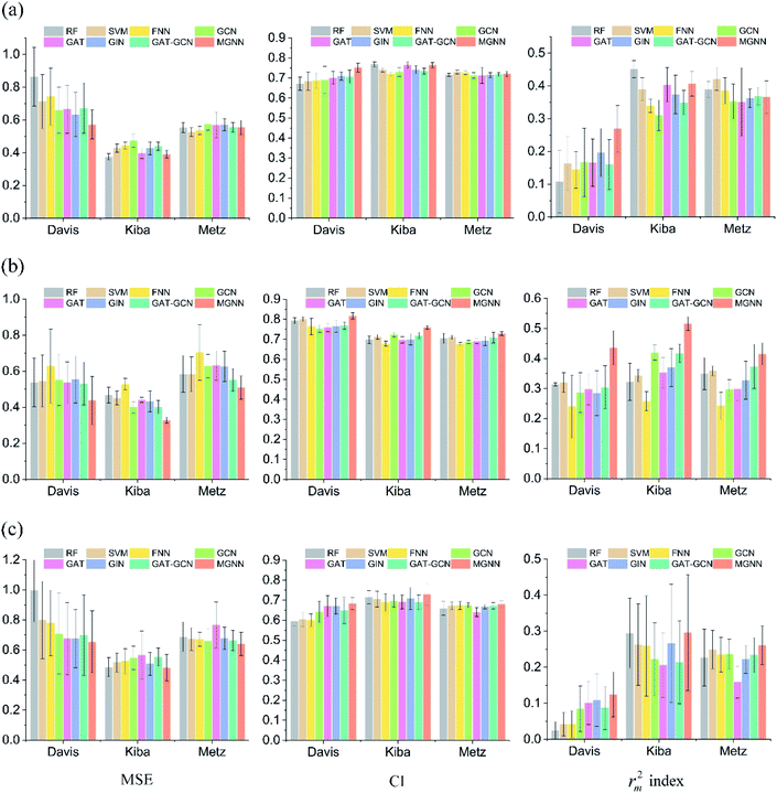
Given that the DTA prediction models are typically used to discover drugs or targets that are absent from the training set, the orphan splits provide realistic and more challenging evaluation schemes for the models. The cluster-based split further prevents the structural information of compounds from leaking to the test set. We compared the proposed MGraphDTA to GraphDTA and three traditional PCM models (RF, SVM, and FNN). For a fair comparison, we replaced the MGNN in MGraphDTA with GCN, GAT, GIN, and GAT–GCN using the source code provided by GraphDTA with the hyper-parameters they reported. We used the five-fold cross-validation strategy to analyze model performance. In each fold, all methods shared the same training, validation, and test sets. Note that the experimental settings remain the same for the eight methods.

Fig. 7 shows the experimental results for eight methods using the orphan-based and cluster-based split settings. Compared with the results using the random split setting shown in Tables 3 and 4, we found that the model's performance decreases greatly in the orphan-based and cluster-based split settings. Furthermore, as shown in Fig. 7(a) and (c), the MSE for MGraphDTA on Davis, KIBA, and Metz datasets using the orphan–drug split were 0.572 ± 0.088, 0.390 ± 0.023, and 0.555 ± 0.043, respectively while those using the cluster-based split were 0.654 ± 0.207, 0.493 ± 0.097, and 0.640 ± 0.078, respectively. In other words, the cluster-based split is more challenging to the DTA prediction model compared to the orphan–drug split, which is consistent with the fact that the cluster-based split setting can prevent the structural information of compounds from leaking to the test set. These results suggest that improving the generalization ability of the DTA model is still a challenge. From Fig. 7(a), we observed that MGNN exceeded other methods significantly in the Davis dataset using the orphan–drug split setting (p < 0.01). On the other hand, there were no statistical differences between MGNN, GAT, and RF (p > 0.05) in the KIBA dataset while these three methods surpassed other methods significantly (p < 0.01). In addition, SVM and FNN methods were superior to other methods significantly in the Metz dataset (p < 0.01). Overall, the traditional PCM models showed impressive results that even surpassed graph-based methods in the KIBA and Metz datasets using the orphan–drug split setting as shown in Fig. 7(a). These results suggest that it may be enough to use simple feature-based methods like RF in this scenario, which is consistent with a recent study.⁶⁴ Since the number of drugs in the Davis dataset is significantly less than that in KIBA and Metz datasets as shown in Table 1, the generalization ability of a model trained on limited drugs can not be guaranteed for unseen drugs. Fig. 8 shows the correlations between predictive values and ground truths of five graph-based models in the Davis dataset using orphan–drug splitting. The predictive value of MGNN was broader than that of other graph-based models as shown in Fig. 8(a). We also noticed that the ground truths and predictive values of MGNN have the most similar distributions as shown in Fig. 8(b). The Pearson correlation coefficients of GCN, GAT, GIN, GAT–GCN, and MGNN for DTA prediction were 0.427, 0.420, 0.462, 0.411, and 0.552, respectively. These results further confirm that MGNN has the potential to increase the generalization ability of the DTA model. From Fig. 7(b), we observed that MGNN outperforms other models significantly in three datasets using the orphan–target split setting (p < 0.01). MGNN also exceeded other methods significantly in KIBA and Metz datasets using the cluster-based split setting as shown in Fig. 7(c) (p < 0.05). It is worth noting that graph-based methods outperformed traditional PCM models in the random split setting as shown in Tables 3 and 4, while the superiority of the graph-based methods was less obvious in the orphan-based and cluster-based split settings as shown in Fig. 7. Overall, the results show the robustness of MGNN in different split setting schemes and prove that both local and nonlocal properties of a given molecule are essential for a GNN to make accurate predictions.

Fig. 7 Comparisons of MGNN and other seven models in Davis, KIBA, and Metz datasets in terms of MSE, CI, and r_m² index (from left to right) using the (a) orphan–drug, (b) orphan–target, and (c) cluster-based split settings.

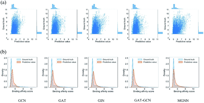Fig. 8 (a) Scatter and (b) kernel density estimate plots of binding affinities between predictive values and ground truths in Davis dataset using the orphan–drug split setting.

3.4 Ablation study

In our designs, the successful construction of the very deep GNN highly relies on dense connection and batch normalization. The dense connection boosts the model performance by alleviating the over-smoothing and vanishing gradient problems, while the batch normalization is able to reduce the over-fitting of very deep models.⁵¹ An ablation study has been conducted to investigate the individual contributions of the dense connection and batch normalization. The experiments were performed from two ends; in the first case we removed the dense connection, and in the second, we removed the batch normalization. Table 6 summarizes the experimental results on the filtered Davis dataset. The results show that both dense connection and batch normalization are necessary for MGNN.

Table 6 Investigating the individual contributions of the dense connection and batch normalization (regression)

Model	RMSE	CI	Spearman
Without dense connection	0.726 (0.008)	0.726 (0.008)	0.620 (0.019)
Without batch normalization	0.746 (0.032)	0.719 (0.014)	0.604 (0.008)
MGraphDTA	0.695 (0.009)	0.740 (0.002)	0.654 (0.005)

---

Furthermore, an ablation study was performed on the filtered Davis dataset to investigate the effect of the receptive field of MCNN on the performance. Specifically, we increased the receptive field gradually by using convolutional layers with a more and more large kernel (i.e., 7, 15, 23, 31). From the results shown in Table 7, it can be observed that the model performance was slightly decreased as increasing the receptive field. Since there are usually a few residues that are involved in protein and ligand interaction,⁶⁵ increasing the receptive field to cover more regions may bring noise information from the portions of the sequence that are not involved in DTA into the model.

Table 7 Impact of max receptive fields of MCNN on filtered Davis dataset (regression)

Max receptive field	RMSE	CI	Spearman
31	0.718 (0.002)	0.732 (0.005)	0.636 (0.013)
23	0.713 (0.008)	0.732 (0.004)	0.635 (0.008)
15	0.710 (0.006)	0.734 (0.005)	0.639 (0.011)
7	0.695 (0.009)	0.740 (0.002)	0.654 (0.005)

---

We also conducted an experiment to show that the MGraphDTA uses both compound and protein information for DTA prediction instead of learning the inherent bias in the dataset as reported in previous studies.^66,67 In particular, we computed the activation values of each unit in the last layer of the two encoders (i.e., and described in Sections 2.3 and 2.4) in the Davis, filtered Davis, KIBA, and Metz datasets, respectively. The higher activation value indicates more contribution of the unit in the model's decision-making.⁶⁸Fig. 9 shows the distribution of these activation values from the protein and ligand encoders. It can be observed that MGraphDTA used both protein and ligand information to make inferences. However, the model was biased toward the protein information in the Davis dataset. The bias is partly due to the unbalanced distribution of binding affinities (labels) of the Davis dataset as shown in Fig. S1† because it is lessened in the filtered Davis dataset as shown in Fig. 9. More precisely, the Davis dataset contains 63 proteins where any drug–target pairs relating to these proteins are labeled with 10 μM bioactivity values (i.e., pK_d value 5). Therefore, a predictive model may simply output binding affinity values around 10 μM for drug–target pairs associated with these proteins, which causes the model biasing toward protein encoder. While these proteins are removed in the filtered davis dataset; thus the bias is alleviated. Another possible reason is that the Davis dataset only contains 68 compounds, which is insufficient to learn a robust drug encoder.

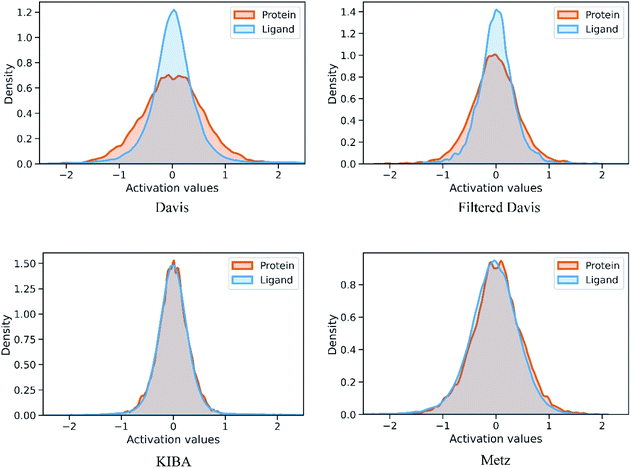Fig. 9 Distribution of activation values of the last layers in the ligand and protein encoders on the Davis, filtered Davis, KIBA, and Metz datasets.

3.5 Grad-AAM provides the visual explanation

Deep learning is usually referred to as the black-box model because it is difficult to trace a prediction back to which features are important. The lack of interpretability limits the applications of deep learning methods, especially in computer-aid drug discovery. Aiming to rationalize the graph-based models, we visualized the atom importance of molecules based on the Grad-AAM. We compared Grad-AAM with graph attention mechanism in the ToxCast dataset to see whether the graph-based models can detect key substructures responsible for certain toxicity or not (also called structural alerts^69,70). We conducted three groups of experiments as follows:

(1) Visualizing MGNN model based on Grad-AAM.

(2) Visualizing GAT model based on Grad-AAM.

(3) Visualizing GAT model based on graph attention mechanism.

Specifically, we first replaced MGNN with a two layers GAT in which the first graph convolution layer had ten parallel attention heads using the source code provided by GraphDTA.³¹ We then trained MGNN-based and GAT-based DTA prediction models under the five-fold cross-validation strategy using the random split setting. Finally, we calculated the atom importance using Grad-AAM and graph attention mechanism and showed the probability map using RDkit.⁴⁸

Table 8 shows the quantitive results of MGNN and GAT. MGNN outperformed GAT by a notable margin (p < 0.01), which further corroborates the superiority of the proposed MGNN. Fig. 10 shows the visualization results of some molecules based on Grad-AAM (MGNN), Grad-AAM (GAT), and graph attention (more examples can be found in ESI Fig. S4 and S5†). According to previous studies,^71–75 epoxide,⁷³ fatty acid,^72,75 sulfonate,⁷¹ and aromatic nitroso⁷⁴ are the structural alerts that correlate with specific toxicological endpoints. We found that Grad-AAM (MGNN) does give the highest weights to these structural alerts. Grad-AAM (MGNN) can not only identify important small moieties as shown in Fig. 10(a)–(d) but also reveal the large moieties as shown in Fig. 10(f), which proves that the MGNN can capture the local and global structures simultaneously. Grad-AAM (GAT) also discerned the structural alerts as shown in Fig. 10(b), (c), (e), and (f). However, Grad-AAM (GAT) sometimes failed to detect structural alerts as shown in Fig. 10(a) and (d) and we might also notice that the highlighted region involves more extensive regions, and does not correspond to the exact structural alerts as shown in Fig. 10(b), (c), and (e). These results suggest that the hidden representations learned by GAT were insufficient to well describe the molecules. On the other hand, the graph attention can only reveal some atoms of structural alerts as shown in Fig. 10(c), (d), and (f). The attention map contained less information about the global structure of a molecule since it only considers the neighborhood of an atom.⁴⁵ The superiority of graph attention was that it can highlight atoms and bonds simultaneously, which the Grad-AAM can only highlight the atoms. Fig. 11 shows the distribution of atom importance for Grad-AAM (MGNN), Grad-AAM (GAT), and graph attention. The distribution for Grad-AAM (MGNN) was left-skewed, which suggested that MGNN pays more attention to some particular substituents contributing most to the toxicity while suppressing the less essential substituents. We also found that Grad-AAM (GAT) tends to highlight extensive atoms from the distribution which was consistent with the results shown in Fig. 10(b), (c), and (e). Conversely, the distribution of graph attention was narrow with most values less than 0.5, which suggested that graph attention often failed to detect important substructures. It is worth noting that some studies utilize global attention mechanisms while dropping all structural information of a graph to visualize a model and may also provide reasonable visual explanations.^46,76 However, these global attention-based methods are model-specific so that the methods can not easily transfer to other graph models. Conversely, Grad-AAM is a universal visual interpretation method that can be easily transferred to other graph models. Moreover, the visual explanation results produced by Grad-AAM may be further improved by applying regularization techniques during the training of MGraphDTA.⁷⁷

Table 8 Comparison results of the proposed MGNN and GAT on the ToxCast dataset (regression)

Model	Proteins	Compounds	MSE	CI	r m ^2 index
GraphDTA	MCNN	GAT	0.215 (0.007)	0.843 (0.005)	0.330 (0.007)
MGraphDTA	MCNN	MGNN	0.176 (0.007)	0.902 (0.005)	0.430 (0.006)

---

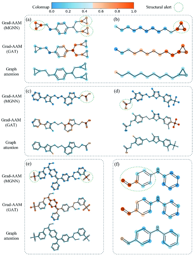Fig. 10 Atom importance revealed by Grad-AAM (MGNN), Grad-AAM (GAT), and graph attention in structural alerts of (a) and (b) epoxide, (c) and (d) fatty acid, (e) sulfonate, and (f) aromatic nitroso.

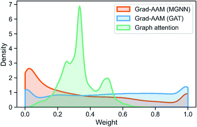Fig. 11 Distribution of atom importance for Grad-AAM (MGNN), Grad-AAM(GAT), and graph attention. Note that we do not consider the bond importance for Grad-AAM (GAT).

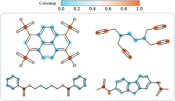
Overall, Grad-AAM tends to create more accurate explanations than the graph attention mechanism, which may offer biological interpretation to help us understand DL-based DTA prediction. Fig. 12 shows Grad-AAM (MGNN) on compounds with symmetrical structures. The distribution of Grad-AAM (MGNN) was also symmetrical, which suggests that representing compounds as graphs and using GNNs to extract the compounds' pattern is able to preserve the structures of the compounds.

Fig. 12 Grad-AAM (MGNN) for molecules with symmetrical structures.

3.6 How does MGNN solve over-smoothing problems?

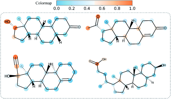
As we mentioned before, the very deep GNN was designed to capture the global and local structures of a compound simultaneously. However, the very deep GNN may cause an over-smoothing representation of vertices. In other words, our quest for a model that is more expressive and aware of the graph structure (by adding more layers so that vertices can have a large receptive field) could be transformed into a model that treats vertices all the same (the vertex representations converging to indistinguishable vectors).⁷⁸ The message passing framework gather feature vectors from neighbors and combine them with the vertex features to update their representation. Therefore, the over-smoothing shows itself in the form of similarity between vertices' embedding. As illustrated in Fig. 13, more and more atoms are included in the calculation of the vertex representation as the model depth is increased. Meanwhile, the vertex embeddings of atom C2 and C1 become more and more similar and we can observe that the only difference in layer 3 is atom C5. Therefore, GNNs may be incapable to distinguish different substructures in a molecule as the model depth is increased. The proposed MGNN addresses the over-smoothing problem by integrating features from different receptive fields for a given vertex or atom as shown in Fig. 4(b). By introducing dense connections into GNN, substructures from different scales of a molecule can be kept despite the increasing model depth. The dense connections also increase the discrimination between each vertex embedding and therefore alleviate the over-smoothing problem. Table 6 shows that the dense connection can improve the model performance significantly (p < 0.01). Fig. 14 shows molecules with similar structures highlighted by Grad-AAM (MGNN). Grad-AAM (MGNN) detected subtle distinctions between the four molecules, which suggests that the MGNN can mitigate the over-smoothing problem.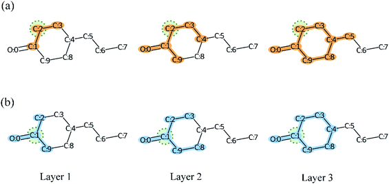

Fig. 13 The receptive field of layer 1, layer 2, and layer 3 of GNN in compound 4-propylcyclohexan-1-one. (a) The receptive field of atom C2. (b) The receptive field of atom C1.

Fig. 14 Grad-AAM (MGNN) for molecules with similar structures.

3.7 Limitations

Although MGraphDTA has shown significant improvements for DTA prediction tasks, there are some limitations in this study. First, this study only focuses on relatively small datasets. We will test MGraphDTA on large-scale datasets^11,12 in future work. Second, it's worth noting that many compounds containing structural alerts are inactive (not having the specific toxicity). In order to determine whether a compound has toxicity to a specific target, we should analyze the drug–target binding mode. Future work will focus on binding mode visualization using Grad-AAM.

4 Conclusion

This work presented a novel graph-based framework based on chemical intuition called MGraphDTA for DTA prediction. MGraphDTA harnessed a MGNN with 27 graph convolutional layers to capture multiscale structures of a molecule and utilized Grad-AAM for visual interpretation. Extensive experiments corroborated the superiority of the proposed method which outperformed the state-of-the-art methods significantly on seven datasets. Moreover, we visualized the atom importance of certain molecules using Grad-AAM from the ToxCast dataset with toxicity as the labels and showed that MGNN was capable of detecting structural alerts. Our results demonstrate that MGraphDTA is a powerful tool to improve the generalization and interpretation capability of DTA prediction modeling.

Code availability

Demo, instructions, and code for MGraphDTA and Grad-AAM are available at https://github.com/guaguabujianle/MGraphDTA.

Data availability

All data used in this paper are publicly available and can be accessed at https://github.com/hkmztrk/DeepDTA/tree/master/data for the Davis and KIBA datasets, https://github.com/cansyl/MDeePred for the filtered Davis dataset, https://github.com/simonfqy/PADME for the Metz dataset and ToxCast datasets, and https://github.com/masashitsubaki/CPI_prediction for the Human and C. elegans datasets.

Author contributions

Calvin Yu-Chian Chen designed research. Ziduo Yang, Weihe Zhong worked together to complete the experiment and analyze the data. Calvin Yu-Chian Chen contributed to analytic tools. Ziduo Yang, Weihe Zhong, Lu Zhao, and Calvin Yu-Chian Chen wrote the manuscript together.

Conflicts of interest

The authors declare that they have no competing interests.

Acknowledgements

This work was supported by the National Natural Science Foundation of China (Grant No. 62176272), Guangzhou Science and Technology Fund (Grant No. 201803010072), Science, Technology & Innovation Commission of Shenzhen Municipality (JCYL 20170818165305521), and China Medical University Hospital (DMR-111-102, DMR-111-143, DMR-111-123). We also acknowledge the start-up funding from SYSU's “Hundred Talent Program”.

References

1. T. Zhao, Y. Hu, L. R. Valsdottir, T. Zang and J. Peng, Brief. Bioinform., 2021, 22, 2141–2150.
2. H. Öztürk, A. Özgür and E. Ozkirimli, Bioinformatics, 2018, 34, i821–i829.
3. H. Lee and J. W. Lee, Arch. Pharm. Res., 2016, 39, 1193–1201.
4. M. Schirle and J. L. Jenkins, Drug Discov. Today, 2016, 21, 82–89.
5. J. Peng, Y. Wang, J. Guan, J. Li, R. Han, J. Hao, Z. Wei and X. Shang, Brief. Bioinform., 2021, 22(5) DOI:10.1093/bib/bbaa430.
6. M. Karplus and J. A. McCammon, Nat. Struct. Biol., 2002, 9, 646–652.
7. Y. Yamanishi, M. Araki, A. Gutteridge, W. Honda and M. Kanehisa, Bioinformatics, 2008, 24, i232–i240.
8. B. J. Bongers, A. P. IJzerman and G. J. P. Van Westen, Drug Discov. Today Technol., 2019, 32, 89–98.
9. G. J. P. van Westen, J. K. Wegner, A. P. IJzerman, H. W. T. van Vlijmen and A. Bender, Medchemcomm, 2011, 2, 16–30.
10. I. Cortés-Ciriano, Q. U. Ain, V. Subramanian, E. B. Lenselink, O. Méndez-Lucio, A. P. IJzerman, G. Wohlfahrt, P. Prusis, T. E. Malliavin, G. J. P. van Westen and others, Medchemcomm, 2015, 6, 24–50.
11. E. B. Lenselink, N. Ten Dijke, B. Bongers, G. Papadatos, H. W. T. Van Vlijmen, W. Kowalczyk, A. P. IJzerman and G. J. P. Van Westen, J. Cheminform., 2017, 9, 1–14.
12. A. Mayr, G. Klambauer, T. Unterthiner, M. Steijaert, J. K. Wegner, H. Ceulemans, D.-A. Clevert and S. Hochreiter, Chem. Sci., 2018, 9, 5441–5451.
13. R. S. Olayan, H. Ashoor and V. B. Bajic, Bioinformatics, 2018, 34, 1164–1173.
14. T. He, M. Heidemeyer, F. Ban, A. Cherkasov and M. Ester, J. Cheminform., 2017, 9, 1–14.
15. Y. Chu, A. C. Kaushik, X. Wang, W. Wang, Y. Zhang, X. Shan, D. R. Salahub, Y. Xiong and D. Q. Wei, Brief. Bioinform., 2021, 22, 451–462.
16. A. Ezzat, M. Wu, X.-L. Li and C.-K. Kwoh, Methods, 2017, 129, 81–88.
17. T. Pahikkala, A. Airola, S. Pietilä, S. Shakyawar, A. Szwajda, J. Tang and T. Aittokallio, Brief. Bioinform., 2015, 16, 325–337.
18. Q. Kuang, Y. Li, Y. Wu, R. Li, Y. Dong, Y. Li, Q. Xiong, Z. Huang and M. Li, Chemom. Intell. Lab. Syst., 2017, 162, 104–110.
19. Y. Chu, X. Shan, T. Chen, M. Jiang, Y. Wang, Q. Wang, D. R. Salahub, Y. Xiong and D.-Q. Wei, Brief. Bioinform, 2021, 22(3) DOI:10.1093/bib/bbaa205.
20. M. Wen, Z. Zhang, S. Niu, H. Sha, R. Yang, Y. Yun and H. Lu, J. Proteome Res., 2017, 16, 1401–1409.
21. A. S. Rifaioglu, R. Cetin Atalay, D. Cansen Kahraman, T. Do\\ugan, M. Martin and V. Atalay, Bioinformatics, 2021, 37(5), 693–704.
22. Z. Wu, B. Ramsundar, E. N. Feinberg, J. Gomes, C. Geniesse, A. S. Pappu, K. Leswing and V. Pande, Chem. Sci., 2018, 9, 513–530.
23. M. K. Gilson, T. Liu, M. Baitaluk, G. Nicola, L. Hwang and J. Chong, Nucleic Acids Res., 2016, 44, D1045–D1053.
24. G. Papadatos, A. Gaulton, A. Hersey and J. P. Overington, J. Comput. Aided. Mol. Des., 2015, 29, 885–896.
25. S. Kim, P. A. Thiessen, E. E. Bolton, J. Chen, G. Fu, A. Gindulyte, L. Han, J. He, S. He, B. A. Shoemaker and others, Nucleic Acids Res., 2016, 44, D1202–D1213.
26. H. Chen, O. Engkvist, Y. Wang, M. Olivecrona and T. Blaschke, Drug Discov. Today, 2018, 23, 1241–1250.
27. H. Altae-Tran, B. Ramsundar, A. S. Pappu and V. Pande, ACS Cent. Sci., 2017, 3, 283–293.
28. H. Öztürk, E. Ozkirimli and A. Özgür, 2019, arXiv Prepr, arXiv1902.04166.
29. I. Lee, J. Keum and H. Nam, PLoS Comput. Biol., 2019, 15, e1007129.
30. A. S. Rifaioglu, E. Nalbat, V. Atalay, M. J. Martin, R. Cetin-Atalay and T. Do\\ugan, Chem. Sci., 2020, 11, 2531–2557.
31. T. Nguyen, H. Le, T. P. Quinn, T. Nguyen, T. D. Le and S. Venkatesh, Bioinformatics, 2021, 37, 1140–1147.
32. M. Karimi, D. Wu, Z. Wang and Y. Shen, J. Chem. Inf. Model., 2020, 61, 46–66.
33. M. Karimi, D. Wu, Z. Wang and Y. Shen, Bioinformatics, 2019, 35, 3329–3338.
34. M. Tsubaki, K. Tomii and J. Sese, Bioinformatics, 2019, 35, 309–318.
35. Q. Feng, E. Dueva, A. Cherkasov and M. Ester, 2018, arXiv Prepr, arXiv1807.09741.
36. W. Torng and R. B. Altman, J. Chem. Inf. Model., 2019, 59, 4131–4149.
37. M. Jiang, Z. Li, S. Zhang, S. Wang, X. Wang, Q. Yuan and Z. Wei, RSC Adv., 2020, 10, 20701–20712.
38. L. Chen, X. Tan, D. Wang, F. Zhong, X. Liu, T. Yang, X. Luo, K. Chen, H. Jiang and M. Zheng, Bioinformatics, 2020, 36, 4406–4414.
39. B. Agyemang, W.-P. Wu, M. Y. Kpiebaareh, Z. Lei, E. Nanor and L. Chen, J. Biomed. Inform., 2020, 110, 103547.
40. Z. Yang, W. Zhong, L. Zhao and C. Y.-C. Chen, J. Phys. Chem. Lett., 2021, 12, 4247–4261.
41. S. Zheng, Y. Li, S. Chen, J. Xu and Y. Yang, Nat. Mach. Intell., 2020, 2, 134–140.
42. G. S. Na, H. W. Kim and H. Chang, J. Chem. Inf. Model., 2020, 60, 1137–1145.
43. G. Li, M. Muller, A. Thabet and B. Ghanem, in Proceedings of the IEEE/CVF International Conference on Computer Vision, 2019, pp. 9267–9276.
44. Y. Li, P. Li, X. Yang, C.-Y. Hsieh, S. Zhang, X. Wang, R. Lu, H. Liu and X. Yao, Chem. Eng. J., 2021, 414, 128817.
45. P. Veličković, A. Casanova, P. Liò, G. Cucurull, A. Romero and Y. Bengio, 6th International Conference on Learning Representations, ICLR 2018 - Conference Track Proceedings, 2018.
46. P. Li, Y. Li, C.-Y. Hsieh, S. Zhang, X. Liu, H. Liu, S. Song and X. Yao, Brief. Bioinform., 2021, 22(4) DOI:10.1093/bib/bbaa266.
47. R. R. Selvaraju, M. Cogswell, A. Das, R. Vedantam, D. Parikh and D. Batra, in Proceedings of the IEEE international conference on computer vision, 2017, pp. 618–626.
48. A. P. Bento, A. Hersey, E. Félix, G. Landrum, A. Gaulton, F. Atkinson, L. J. Bellis, M. De Veij and A. R. Leach, J. Cheminform., 2020, 12, 1–16.
49. J. Gilmer, S. S. Schoenholz, P. F. Riley, O. Vinyals and G. E. Dahl, in International Conference on Machine Learning, 2017, pp. 1263–1272.
50. C. Morris, M. Ritzert, M. Fey, W. L. Hamilton, J. E. Lenssen, G. Rattan and M. Grohe, in Proceedings of the AAAI Conference on Artificial Intelligence, 2019, vol. 33, pp. 4602–4609.
51. K. He, X. Zhang, S. Ren and J. Sun, in European conference on computer vision, 2016, pp. 630–645.
52. G. Huang, Z. Liu, L. Van Der Maaten and K. Q. Weinberger, in Proceedings of the IEEE conference on computer vision and pattern recognition, 2017, pp. 4700–4708.
53. Z. Yang, L. Zhao, S. Wu and C. Y.-C. Chen, IEEE J. Biomed. Heal. Informatics, 2021, 25, 1864–1872.
54. J. T. Metz, E. F. Johnson, N. B. Soni, P. J. Merta, L. Kifle and P. J. Hajduk, Nat. Chem. Biol., 2011, 7, 200–202.
55. J. Tang, A. Szwajda, S. Shakyawar, T. Xu, P. Hintsanen, K. Wennerberg and T. Aittokallio, J. Chem. Inf. Model., 2014, 54, 735–743.
56. M. I. Davis, J. P. Hunt, S. Herrgard, P. Ciceri, L. M. Wodicka, G. Pallares, M. Hocker, D. K. Treiber and P. P. Zarrinkar, Nat. Biotechnol., 2011, 29, 1046–1051.
57. D. P. Kingma and J. L. Ba, 3rd International Conference on Learning Representations, ICLR 2015 - Conference Track Proceedings, 2015.
58. T. Akiba, S. Sano, T. Yanase, T. Ohta and M. Koyama, in Proceedings of the 25th ACM SIGKDD international conference on knowledge discovery & data mining, 2019, pp. 2623–2631.
59. M. Gönen and G. Heller, Biometrika, 2005, 92, 965–970.
60. K. Roy, P. Chakraborty, I. Mitra, P. K. Ojha, S. Kar and R. N. Das, J. Comput. Chem., 2013, 34, 1071–1082.
61. F. Pedregosa, G. Varoquaux, A. Gramfort, V. Michel, B. Thirion, O. Grisel, M. Blondel, P. Prettenhofer, R. Weiss, V. Dubourg and others, J. Mach. Learn. Res., 2011, 12, 2825–2830.
62. A. Paszke, S. Gross, F. Massa, A. Lerer, J. Bradbury, G. Chanan, T. Killeen, Z. Lin, N. Gimelshein, L. Antiga, A. Desmaison, A. Köpf, E. Yang, Z. DeVito, M. Raison, A. Tejani, S. Chilamkurthy, B. Steiner, L. Fang, J. Bai and S. Chintala, Adv. Neural Inf. Process. Syst., 2019, 32, 8026–8037.
63. A. Airola and T. Pahikkala, IEEE Trans. neural networks Learn. Syst., 2017, 29, 3374–3387.
64. Q. Ye, C.-Y. Hsieh, Z. Yang, Y. Kang, J. Chen, D. Cao, S. He and T. Hou, Nat. Commun., 2021, 12, 6775.
65. B. K. C. Dukka, Comput. Struct. Biotechnol. J., 2013, 8, e201308005.
66. L. Chen, A. Cruz, S. Ramsey, C. J. Dickson, J. S. Duca, V. Hornak, D. R. Koes and T. Kurtzman, PLoS One, 2019, 14, e0220113.
67. J. Sieg, F. Flachsenberg and M. Rarey, J. Chem. Inf. Model., 2019, 59, 947–961.
68. C. Cao, X. Liu, Y. Yang, Y. Yu, J. Wang, Z. Wang, Y. Huang, L. Wang, C. Huang, W. Xu and others, in Proceedings of the IEEE international conference on computer vision, 2015, pp. 2956–2964.
69. Z. Wu, D. Jiang, J. Wang, C.-Y. Hsieh, D. Cao and T. Hou, J. Med. Chem., 2021, 64, 6924–6936.
70. A. Mukherjee, A. Su and K. Rajan, J. Chem. Inf. Model., 2021, 61, 2187–2197.
71. M. D. Barratt, D. A. Basketter, M. Chamberlain, G. D. Admans and J. J. Langowski, Toxicol. Vitr., 1994, 8, 1053–1060.
72. A. S. Kalgutkar and J. R. Soglia, Expert Opin. Drug Metab. Toxicol., 2005, 1, 91–142.
73. M. P. Payne and P. T. Walsh, J. Chem. Inf. Comput. Sci., 1994, 34, 154–161.
74. J. Kazius, R. McGuire and R. Bursi, J. Med. Chem., 2005, 48, 312–320.
75. V. Poitout, J. Amyot, M. Semache, B. Zarrouki, D. Hagman and G. Fontés, Biochim. Biophys. Acta, Mol. Cell Biol. Lipids, 2010, 1801, 289–298.
76. Z. Xiong, D. Wang, X. Liu, F. Zhong, X. Wan, X. Li, Z. Li, X. Luo, K. Chen, H. Jiang and others, J. Med. Chem., 2019, 63, 8749–8760.
77. R. Henderson, D.-A. Clevert and F. Montanari, in Proceedings of the 38th International Conference on Machine Learning, ed. M. Meila and T. Zhang, PMLR, 2021, vol. 139, pp. 4203–4213.
78. K. Oono and T. Suzuki, 2019, arXiv Prepr, arXiv1905,10947.

---

Footnotes

† Electronic supplementary information (ESI) available: Details of machine learning construction, vertex features of graphs, data distributions, hyperparameters tuning, and additional visualization results. See DOI: 10.1039/d1sc05180f

‡ Equal contribution.

---