A coupled reinforcement learning and IDAES process modeling framework for automated conceptual design of energy and chemical systems

Abstract

Computer-aided process engineering and conceptual design in energy and chemical engineering has played a critical role for decades. Conventional computer-aided process and system design generally starts with process flowsheets that have been developed through experience, which often relies heavily on subject matter expertise. These widely applied approaches require significant human effort, either providing the initially drafted flowsheet, alternative connections, or a set of well-defined heuristics. These requirements not only limit the flexibility of the flowsheet design process, but also make the system design highly reliant on the engineer's experiences and expertise. In this study, a novel reinforcement learning (RL) based automated system for conceptual design is introduced and demonstrated on the Institute for the Design of Advanced Energy System (IDAES) Integrated Platform. IDAES is an open-source platform with extensible libraries of dynamic unit operations and thermophysical property models. It provides the capability of optimizing energy and chemical process flowsheets with state-of-the-art solvers and solution techniques. The RL approach provides a generic tool for identifying process configurations and significantly decreases the dependence on human intelligence for energy and chemical systems conceptual design. An artificial intelligence (AI) agent performs the conceptual design by automatically deciding which process-units are necessary for the desired system, picking the process-units from the candidate process-units pool, connecting them together, and optimizing the operation of the system for the user-defined system performance targets solely according to the reward system, while the reward system can incorporate user's experiences and knowledge to advance the training process. The AI agent automatically interacts with the physics-based system-level modeling and simulation toolset IDAES to guarantee the system design is physically consistent. This study showcases the application of the RL-IDAES framework through two demonstration cases. These cases prove the framework's capability of designing and optimizing complicated systems with high flexibility at affordable computing costs. To illustrate, designing the hydrodealkylation of toluene system from 14 candidate process-units yielded 123 feasible designs within 20 hours on a standard PC. Moreover, the framework's versatility is demonstrated by the ability to transfer a trained RL model to different training cases, thus enhancing the overall performance of the reinforcement learning process.

---

1. Introduction

Computer-aided process engineering and conceptual design have become an important field that has played a critical role in chemical engineering and industry.^1,2 The widely used computer-aided process design and process intensification approaches mostly rely on physics-based, system-level simulations. This means that the system design flowsheets are mostly user-provided, and the simulation-based computer-aided design tools provide the estimation of the system performance and the optimization for the specific flowsheet configuration.^3–6 The researchers can adjust the design according to the estimation of the system performance, and iterate by evaluating multiple potential designs or process configurations.^2,7

The computer-aided system design without a prior deterministic flowsheet is much more challenging.⁸ The concept of superstructure optimization is one of the popular procedures that does not need a specific flowsheet⁹ but needs a large set of process alternatives,^10,11 and is often used with simplified mathematical representations of chemical operations. Another popular approach for non-deterministic flowsheet automated design is the evolutionary modification method. It needs an initial drafted flowsheet, and this evolutionary modification approach can analyze and change one or more connections in the flowsheet to improve it, until no further improvement in the flowsheet can be made.¹² The third widely used automated flowsheet design approach is called systematic generation, which creates a flowsheet sequentially by adding units one by one from heuristics. The heuristics are constructed based on prior knowledge.¹³ Hence, the widely applied approaches mentioned above still require significant human efforts, either providing the initial drafted flowsheet, alternative connections, or a well-defined heuristics data set. These requirements not only limit the flexibility of the flowsheet design, but also make the system design highly reliant on the engineer's experiences and expertise.

Machine learning (ML) has developed rapidly in the past decades and has shown promising advantages in the applications of reduced order model,^14,15 image and video processing,^16–19 and natural language processes.²⁰ Among various ML algorithms, reinforcement learning shows great potential as an alternative to human beings' intelligence and creativity,^21,22 such as playing games and self-driving cars. RL focuses on how intelligent agents should take actions in an environment in order to maximize the cumulative reward.²¹ The true advantage of RL is that it does not need existing training data sets, such as labeled input–output pairs and/or sub-optimal actions database.²¹ Additionally, RL is also flexible in learning from existing labeled examples and then combined with unsupervised self-learning to accelerate the accumulation of knowledge.²³ In recent years, some pioneering efforts have been made in applying RL to conceptual designs of energy and chemical systems. Khan et al. used hierarchical reinforcement learning to search for optimal processing routes for hydrogen production and steam methane reforming.^24,25 Gottl et al. applied RL to sequentially build synthesis flowsheets with a specific process problem.^26–28

In this study, an RL-based automated conceptual design approach is introduced and demonstrated by interacting with a general energy system modeling platform, the Institute for the Design of Advanced Energy System Integrated Platform (24). The RL approach significantly decreases the requirements from human interaction for energy and chemical system design. The user decides the candidate process-units pool (CPP) from the IDAES module library, which provides all the available energy and chemical operations (e.g., phase change, temperature change, pressure change, etc.) that are allowed to be used in the system. An artificial intelligence agent can then automatically decide which process-units are necessary for the desired system, pick the units from the CPP, connect them together, actively interact with the environment and optimize the system design for the user-defined system performance targets. IDAES serves as the environment to guarantee the system designs are physically consistent. IDAES provides extensive equation-based models of unit operations and thermophysical properties, as well as capabilities of optimizing process flowsheets with state-of-the-art solvers. The interactive framework is named RL-IDAES in this study. The proposed RL-IDAES framework is designed to be generic and can be adapted to different energy and chemical engineering systems, and the user can specify system complexity and optimization objectives. Two case studies are presented in this manuscript to demonstrate the capability of the RL-IDAES and the transferability of the trained AI agent among different conceptual designs.

2. Methodology

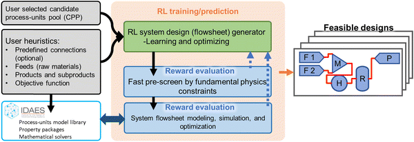
The workflow of the RL-guided energy and chemical systems design framework (RL-IDAES) is shown in Fig. 1. As the left portion of Fig. 1 shows, two inputs are defined by the user. The first one is the process-units pool that is available for RL to construct system designs. The second one is the user heuristics. It includes the system raw material feeds, the expected system products and potential subproducts, and the expectations for the desired system, such as higher product flow rate, higher product purity, higher revenue, lower energy cost, and so on. The user can also provide additional knowledge, such as certain predefined connections for the system, which may help the RL on reducing the search space and increasing the success rate of system design. These user-predefined connections are optional. The center core portion of the framework, as shown in Fig. 1, is the RL training and prediction framework. The RL flowsheet generator keeps proposing new system designs and sends them into the reward evaluation part. There are two steps of reward evaluation. The first step is the fast pre-screen according to fundamental physics constraints, and the second step is the system-level modeling, simulation, and optimization in IDAES, as shown in the two-direction arrow marked in Fig. 1. The detailed explanations about the reward evaluations are in Section 2.1. The RL flowsheet generator receives the reward as the blue dash line arrow shown in Fig. 1, and proposes new designs according to the received reward through a trained deep neural network (DNN). The detailed explanations of how the rewards are utilized for training the DNN and how the DNN helps on adjusting and proposing new flowsheets are in Section 2.2. With adequate training of the DNN, the RL framework can generate a series of feasible system designs that are physically operational and meet the user-desired system performance targets.

Fig. 1 The workflow of the RL-guided energy and chemical system design framework.

2.1 Environment feedback for rewards

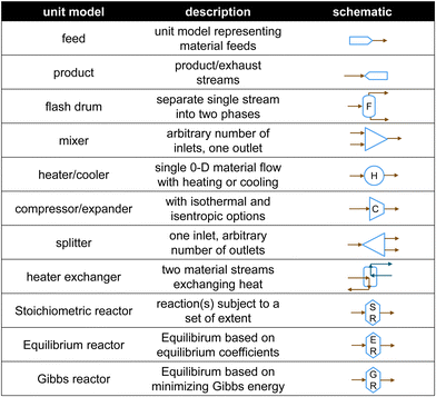
For constructing the RL framework that is more flexible and compatible with any potential desired systems, there are no integrated pre-defined system design rules in the RL AI agent. The AI agent can connect any outlet to any inlet of the process units without any direct restrictions. Additionally, the reward evaluation system and procedure are also not seeable to the AI agent. What the AI agent can receive and learn from is feedback reward scores only.

2.1.1 IDAES integrated platform for system-level optimization. This work leverages the IDAES Integrated Platform to evaluate and optimize the configurations proposed by the AI agent (described in Section 2.2). IDAES is an open-source platform developed by a multi-lab collaboration led by the National Energy Technological Laboratory (NETL) of the United States Department of Energy (DOE) to accelerate the design, development, and optimization of advanced energy systems.^29–31 It is built on the foundation of an open-source algebraic modeling environment, Pyomo, and is capable of formulating, initializing and solving optimization problems within the Python ecosystem while accessing numerous Python libraries for data analysis and visualization.^32,33

IDAES includes a large process-unit model library of typical unit operations such as feeds, products, mixers, splitters, flash drums, heat exchangers, and stoichiometric reactors (Fig. 2). The library is continually being updated and includes advanced energy models such as solid oxide fuel cells, auto-thermal reforming, air separation units, steam cycle, boiler models, and steam turbines. Each model provides a set of equations describing a given operation (e.g., phase change, temperature change, pressure change, chemical reactions), and every model and equation is editable and extensible. The user can add, remove or modify variables and constraints for these unit models. This level of flexibility allows the RL-IDAES to be applied to a wide range of conceptual design problems, enabling modelers to develop and customize the flowsheet to their needs.²⁹

Fig. 2 Common process units in IDAES Integrated Platform.

By integrating the extensible model library and advanced optimization-based approaches, the IDAES platform can be used for designing novel, large-scale, complex systems with dynamic optimization under uncertainty. The optimization objective can be a thermophysical property (e.g., flow rate, temperature, reaction rate, etc.) or any complex continuous quantification parameter (e.g., annual revenue, product purity, etc.).

2.1.2 Immediate-reward system with physics constraints. With the IDAES Integrated Platform, AI agent's actions can be converted to draft flowsheets. Ideally, every flowsheet, even incomplete, is supposed to be evaluated by IDAES simulation and optimization and then assigned a reward. However, it is not only difficult but also inefficient to evaluate any infeasible flowsheet. Feasible energy and chemical systems must follow some fundamental and general rules or physics constraints. Based on these constraints, an immediate-reward system or fast pre-screen process can be built to evaluate draft flowsheets before sending them to the IDAES. Ten fundamental physics constraints are considered in the process, as shown in Fig. 3. For example, Constraint 2 is implemented to avoid repeated use of one inlet or outlet, and Constraint 10 ensures all connected units are in one system. These are general rules desired by any conceptual system design. Each fundamental physics constraint is associated with a specific penalty. As one flowsheet goes through the immediate-reward system, it gets penalties for violating each physics constraint and obtains a deducted reward. Violating certain physics constraints (e.g., Constraints 1 and 2) or connecting one inlet to an inactive outlet leads building an appropriate flowsheet impossible, thus triggering the early-termination mechanism, which assigns the flowsheet the minimum reward and ends the iteration/episode. At the early stage of the training, the agent makes selections randomly with no bias or information and frequently causes early terminations, which drives the AI agent to learn to avoid inappropriate connections in priority.

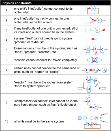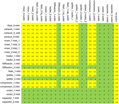
Fig. 3 Physics constraints energy or chemical systems must follow (H, R, C, F, O in the plot denote heater, reactor, compressor, flash drum and any other unit).

This immediate-reward system enables the RL-IDAES to evaluate any incomplete flowsheet; therefore, the flowsheet-building process doesn't have to be sequential. As the AI agent is not learning promising routes to build optimal flowsheets but learning essential connections, it can handle complex and large-scale systems with multiple system inlets and recycling loops. The immediate-reward system also has a mechanism to control the “system complexity” or how complicated the user wants the RL-found designs to be. This function is realized by issuing a “no action” penalty when the agent picks the “no action” option from the action space. A higher penalty should encourage the agent to take an “active” option instead of “no action”. Please note that the AI agent is blind to the rules in the immediate-reward system or the fast pre-screen process. The AI agent can only receive and learn from feedback reward scores.

2.1.3 Finalized-reward system with IDAES integrated platform. Suppose one flowsheet satisfies all the physics constraints in Fig. 3. In that case, it is considered a “complete” flowsheet and will be further evaluated by the IDEAS integrated platform. IDAES will determine if the flowsheet is feasible (physically operational) and re-evaluate it with a reward associated with the optimization objective (e.g., product purity, system revenue, etc.). In this proposed RL-IDAES framework, IDAES provides two levels of feedback to the AI agent. One is the feasibility of the draft system flowsheet through physics-based simulation and optimization. The second one is the optimization of operational and property parameters of all the connected process-units to achieve the optimal system performance with the draft flowsheet and the user-desired objective. An infeasible flowsheet will inherit the evaluation result of the immediate-reward system. A feasible flowsheet will be assigned the maximum reward, plus an extra reward for excellent system performance. The case demonstration section (Section 3) will show more details about assigning reward to the IDAES flowsheet.

The AI agent takes actions solely according to the reward system. One thing to be noted is although the proposed RL-IDAES is an automated conceptual design framework, it can always incorporate engineers' knowledge and experiences by adding them into the immediate-reward or finalized-reward systems to advance the training process.

2.2 Reinforcement learning algorithm and framework

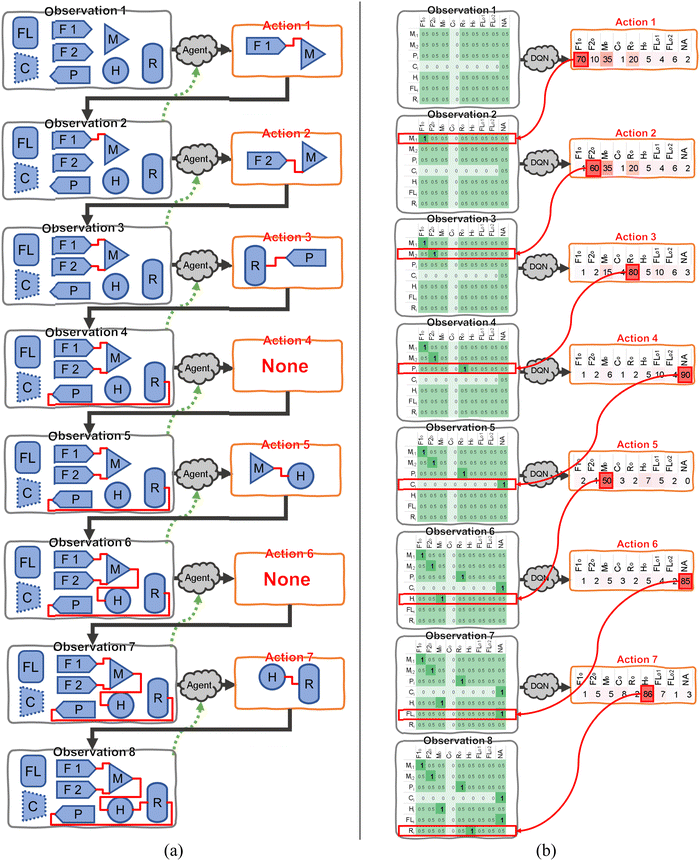
The sketch of the concept of the RL-guided energy and chemical system design is shown in Fig. 4(a). The observation comprises all the energy and/or chemical process-units and their connections. For example, as shown in Fig. 4(a), the “Observation 1” includes the available process-units. They are raw material feed #1 (F1), raw material feed #2 (F2), product (P), mixer (M), heater (H), reactor (R), compressor (C), and flash (FL), as marked in Fig. 4(a). Please note that the process units shown in Fig. 4(a) are only for the sake of illustration of the procedure, and practical observations may include many more process-units. The user can choose whether certain process-units are active, which are named the candidate process-units pool in this study. It means the RL can select a unit in CPP and connect it into the system. The compressor (C) shown in Fig. 4(a) is edged with the dotted line, which means this compressor is deactivated by the user.

Fig. 4 Sketch of the concept of the RL-guided energy and chemical system design. (a) the steps shown by the connections of process-units; (b) the corresponding matrix for DQN inputs and outputs that represent the connections of process-units.

Initially, there is no connection between any process-units. The agent decides an action according to the reward evaluation of the current observation, such as connecting the raw material feed #1 to the mixer, as “Action 1” shown in Fig. 4(a). After “Action 1”, the current observation is updated to a new observation, as shown in “Observation 2” in Fig. 4(a). An immediate-reward system is used to evaluate the connections in “Observation 2”, and assign a reward, which is then sent back to the agent, as the green dash line shown in Fig. 4(a). The immediate-reward system and associated evaluation of rewards are discussed in Section 2.1. Following this procedure, the candidate process-units can be connected one by one until a fully connected system flowsheet is acquired. Note that it is unnecessary to use all the units in the CPP for a completed system flowsheet design, for example, excluding the flash (FL) in Fig. 4(a). The agent is allowed to do nothing for any step of action, as “Action 4” and “Action 6” are shown in Fig. 4(a). Also, the agent doesn't have to build a flowsheet sequentially from system inlets to system products/exhausts.

At the beginning of training, the agent cannot distinguish between the correct and incorrect connections and makes random selections with no bias or information, which usually causes the connected flowsheet to be physically infeasible or far from the user's expected system performance. The agent can learn and improve the decision of selecting the connections according to the reward system. By tracking the potential directions of increasing the finalized reward, the agent would be well trained, and find optimized system flowsheet designs. Based on this training scheme, the deep Q value network (DQN) is applied to the RL framework in this study.

2.2.1 Observation data structure and action implementation. To utilize the DQN to learn, search, and optimize the system design, the observations and actions are transformed into the data structure, as shown in Fig. 4(b), which is consistent with the sketched example in Fig. 4(a). The abbreviations in Fig. 4(b) for process-unit's names are the same as the ones defined in Fig. 4(a). The subscript i and o stands for the inlet and outlet respectively. The subscript i1, i2, o1, and o2 represent the inlet #1, inlet #2, outlet #1, and outlet #2 if the process-units have multiple inlets and/or outlets. The observation is defined as a 2-dimensional (2D) array. The columns of the array represent all the outlets of the available process-units, with an additional column representing “no action”, and the rows of the array represent all the inlets of the available process-units. The raw material feed is considered a process-unit, but only has one outlet, and no inlet. The system product and exhaust are also considered process-units, but only have one inlet, and no outlet. Other functional process-units should have either one or more inlets/outlets. If one process-unit is activated by the user, the values in the corresponding column and row are initialized as 0.5. If one unit is deactivated by the user, the values in the corresponding column and row are initialized as 0, as the compressor's inlet and outlet shown in Fig. 4(b). The RL agent will move from the top to the bottom row step by step, connecting the inlet to one of the outlets in each row.

The action space is a 1-dimensional (1D) vector, and the elements in this vector represent all the outlets, as shown in Fig. 4(b). The value in each element is the Q value of picking a certain outlet. The Q value is defined as

Q = R + γ·max(Q_next), (1)

where, R is the immediate reward of taking the action, γ is the decay factor, Q_next is the set of future Q values, and max() selects the maximum value among the future Q values. More details for applying eqn (1) are discussed in Section 2.2.2. The action is picking the process-unit's outlet with the highest Q value, and connecting it into the system. According to the 2D array observation, the DQN can predict the Q values for each action option. The action is applied to the observation array row by row, as the red blocks shown in Fig. 4(b). For example, “Action 1” in Fig. 4(b) shows the “feed 1 outlet” has the highest Q value of 70. Then, the “feed 1 outlet” in the first row in the observation array is picked, and its value is updated to 1, as the “Observation 2” shown in Fig. 4(b). This “row by row” strategy reduces the action space size; otherwise, the action space needs to be equivalent to the observation array, which will significantly increase the complexity and difficulty of training the DQN. The “no action” is also one of the options in the action space, as “Action 4” shown in Fig. 4(b). If the “no action” is picked, the column “no action” in the observation array will be updated to 1, as “Observation 5” shows. This “no action” column in the observation array is critical for training the DQN. If there is no such column, “Observation 4” and “Observation 5” are the same, and the DQN is confused about which row should be working on. The values 0, 0.5, and 1, representing the three statuses (inactive, active and connected), are selected for two purposes. One is making the values in the observation matrix between 0 and 1, without further normalization. The other is that the differences among the statuses are as big as possible, which helps the DQN identify them even after passing layers of neural networks.

2.2.2 Deep Q value network structure and training. The DQN is a multi-layer neural network that builds the connection between observation data and the Q value data, as shown in Fig. 5. The input for the DQN is the observation array, and the output from the DQN is the Q value vector. The DQN includes four convolutional neural network (CNN) layers that extract the key features from the observation and compress them into a smaller 3D array. The last convolutional layer is flattened into a 1D array and connected to two fully connected layers. When the observation array is large, including the convolutional layers can usually increase the DQN prediction accuracy. If the observation array is very small, such as smaller than 8 × 8, the convolutional layers may not be necessary. The observation array can be flattened, and directly connected to fully connected layers.

Fig. 5 Sketch of the structure of DQN.

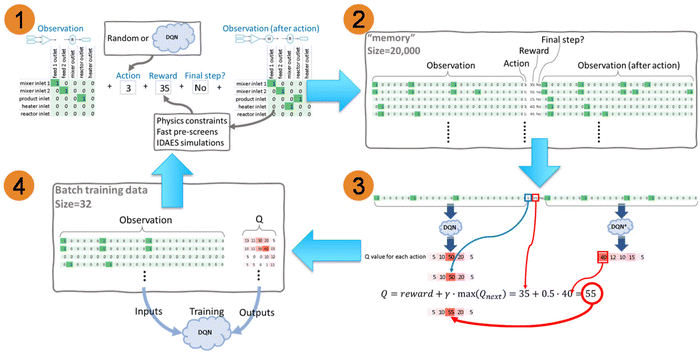
Because there are no existing prior system designs and/or data available to train the DQN, the RL has to generate the draft designs all by itself, and use these draft designs to train itself. The main procedures are shown in Fig. 6. Fig. 6 (part 1) records the raw attempts of connecting process-units. According to the “Observation” in part 1, which is a 2D array as discussed in Section 2.1.2, an action #3 is selected. This action index can be randomly picked or predicted by the DQN. A greedy factor ε, whose value is between 0 and 1, is used to control whether an action is randomly picked or DQN predicted. Before every action, a random number δ, which is between 0 and 1, is generated. If δ > ε, an action is randomly picked. If δ < ε, an action is decided by the DQN prediction. ε is gradually increasing from 0 to 1 with RL training. This means that, at the beginning of the training, the DQN has limited knowledge or experience in predicting the correct action, so a random action is preferred. With the training progress, the action has a higher and higher probability of being determined by DQN prediction.

Fig. 6 The steps of preparing data set and training DQN.

An example is shown in Fig. 6 (part 1): the action #3 stands for the “mixer outlet”, and it should be applied on the 4th row of the observation array, so it is connected to the “heater inlet” and yields the “New observation (after action)”. The “New observation” is then evaluated by a series of physics constraints for fast pre-screens, then through IDAES system-level modeling and optimization,²⁹ if the connected system can pass all the fast pre-screens. The fast pre-screens and the IDAES simulation and optimization can provide the rewards of this action. For this sketched demonstration, the reward is 35, as shown in Fig. 6 (part 1). The details about the fundamental physical constraints and IDAES simulation and optimization are discussed in Section 2.1. Whether this action is the final step for connecting a system is also recorded. In this sketched demonstration, it is not the final step yet, as shown in Fig. 6 (part 1). A process-unit is still available in the 5th row of the observation array, which is the “reactor inlet”.

By repeating the steps in part 1, a large number of raw attempts are recorded into “memory” as part 2 shown in Fig. 6. The “Observation” and the “New observation” 2D arrays are flattened into a 1D array in the “memory”. Therefore, all the necessary data associated with one action is recorded in one row. The recorded “memory” is not infinitely large and is usually defined as around 10 000 to 100 000 rows. The new raw attempts data overwrite the old data in the memory. Because the newer data usually focuses on the attempts of connection that can get higher rewards, it is unnecessary to keep the older data, which is usually more random and less meaningful. This limited “memory” size can effectively increase the DQN training efficiency.

Usage of all the data in memory to train the DQN, which could be computationally expensive, is not necessary. After the RL attempts to construct 10 to 100 system flowsheets, which is called training interval, the DQN will be trained. A small batch of “memory” is randomly picked for training. The batch size is usually defined as 30 times the training interval, defined by the user from 10 to 100. In the small batch, each row of data needs to be converted to the Q values, as the steps shown in Fig. 6 (part 3). Both “Observation” and “New observation” arrays are sent to DQN and DQN* for predicting the Q values. The structure of the DQN and DQN* are the same, and the parameters in DQN* are not trained, but directly copied from DQN with a delay. The feature of delay is mainly for stabilizing the RL framework. As shown in the sketch demonstration in Fig. 6 (part 3), the predicted Q values for the 5 action options based on “Observation” are [5, 50, 17, 20, 5], and the Q values for “New observation” are [40, 12, 10, 15, 5], which is defined as Q_next. The maximum value in Q_next is 40. In this recorded row, the action reward is 35. Using eqn (1) with γ = 0.5, the new Q value can be calculated as 35 + 0.5 × 40 = 55. In this recorded row, the action is 3, therefore this updated Q value 55 only replaces the value 17 in the 3rd element in the Q vector, and leaves other values unchanged, as the blue block marked in Fig. 6 (part 3). The new Q vector then becomes [5, 50, 55, 20, 5]. If the element in the recorded row representing the indicator of “Final step” is “Yes”, which means there is no further action needed, there is no Q_next, and eqn (1) is simplified to Q = reward. Please note that, the recorded action number is not necessary the same as the index of the maximum Q value. As shown in this sketch example in Fig. 6 (part 3), the maximum Q value is 50, and its index is 2nd, but the recorded action is 3. There are two reasons that lead to this situation. The first reason is that the action may be randomly picked when recorded. The second reason is that the DQN has been updated, and its prediction is not the same as the ones from the old DQN, when the action was recorded.

By implementing the calculations in Fig. 6 (part 3), all the data in the batch memory can be converted to the format of observation and Q array, as shown in Fig. 6 (part 4). The Root Mean Squared Propagation (RMSProp) algorithm^34,35 is used to optimize the parameters in DQN, with learning rate α = 0.01. RMSProp is one of the most popular optimizers for neural networks training, and provides the balanced performance between robustness and convergence speed. The observation and the Q array, as the inputs and outputs respectively, are used to train the DQN to update its parameters. By looping parts 1 to 4, the DQN can be kept updated, and the recorded system connection should get closer and closer to the targeted, optimized system design.

3. Results and discussions

Two demonstration case studies are presented in this section to show how the AI agent solves the conceptual design problem. The first one is the production of Benzene with Hydrodealkylation (HDA) reaction, which is discussed in Section 3.1 and named RL-HDA for short. The second one is the methanol synthesis system, discussed in Section 3.2 and named RL-methanol for short. The AI agent takes actions to build flowsheets, runs IDAES to optimize each flowsheet, and assigns rewards to actions. Section 3.2 also presents the RL framework's network transferability. The RL can reduce computing costs and improve training performance by loading a trained DQN of the same or a different system. A few issues mentioned in Sections 3.1 and 3.2 are resolved with continuing training in Section 3.3.

3.1 Hydrodealkylation of toluene

The RL framework is utilized to design a chemical system to produce benzene with a hydrodealkylation reaction.³⁶ In this study, the HDA reaction involves reacting an aromatic hydrocarbon with hydrogen gas at a high temperature to form Benzene as follows:

C₆H₅CH₃ + H₂ → C₆H₆ + CH₅ (2)

The desired chemical system uses 0.3 mol s⁻¹ of hydrogen, 0.3 mol s⁻¹ of toluene and 0.02 mol s⁻¹ of methane as raw materials with a temperature of 303.2 K and a pressure of 350 000 Pa. The objective is to develop a flowsheet that maximizes the Benzene flow rate while achieving the highest Benzene purity. Typically, such a process requires a dedicated reactor operation to carry out the conversion step, as well as upstream processes to bring feeds to reactor conditions and downstream processes for heat and product recovery. Process optimization typically involves a tradeoff between operating costs. For example, a process may use a fired heater to pre-heat the feed stream rather than assuming a colder reactor feed and supplying heat directly to the reactor. Similarly, a process may utilize a post-reactor expander or cooler to achieve optimal recovery conditions or assume temperature and pressure drop in the flash drum itself. By allowing all reasonable design options, the AI agent accounts for these tradeoffs and lets the algorithm make these decisions.

3.1.1 Initialization and reward assignment. From the IDAES-provided common process-unit models library (Fig. 2), 2 to 3 of almost every category of the fundamental process-units, which are commonly used in chemical synthesis system, are picked as the maximum available unit pool, as listed in the last row of Table 1. Please note that there is no strict rule for choosing process-units or not for the maximum available unit pool. A smaller pool size usually helps the AI agent focus on the useful process-units. Including too many distracting units would slow down the AI agent training. In this example, 22 process-units are picked for the maximum available unit pool. Then, the user can choose to activate or deactivate certain process-units in this maximum available unit pool to composite the user-defined candidate units pools. The observation template is built accordingly, with 21 rows corresponding to 21 inlets, 22 columns corresponding to 21 outlets and the “no action” column. The user selects some available units as the candidate units pool for the AI agent to build with. To test the robustness of the RL framework, seven different CPPs were selected to be evaluated. These CPPs consist of 14 to 20 process-units and are described in Table 1, and are named as HDA-14 to HDA-20 for short. For example, the HDA-16 contains two feeds, one product, two exhausts, three mixers, two compressors, two heaters, one reactor, two flash and one splitter. The flowsheets/observations are initialized as shown in Fig. 7. 15 rows and 15 columns corresponding to 16 units are initialized as “active” with a value of 0.5 (yellow highlighted). The other spots are initialized as “inactive” with a value of 0 (green highlighted).

Table 1 Potential candidate process-units pools for HDA demonstration

No. of units	Name	Feed	Product	Exhaust	Mixer	Compressor	Heater	Reactor	Flash	Splitter	Cooler	Expander
14	HDA-14	2	1	2	2	1	1	1	1	1	1	1
15	HDA-15	2	1	2	2	2	2	1	2	1
16	HDA-16	2	1	2	3	2	2	1	2	1
17	HDA-17	2	1	2	3	2	2	1	2	2
18	HDA-18	2	1	2	3	2	2	2	2	2
19	HDA-19	2	1	2	3	2	2	2	2	2	1
20	HDA-20	2	1	2	3	2	2	2	2	2	1	1
22 (All)		2	1	2	3	2	2	2	2	2	2	2

---

Fig. 7 Initialized flowsheet when 16 units are selected as CPP.

In each iteration or episode, the AI agent will move from the top to the bottom row, connecting one inlet to one outlet in each step. There will be five kinds of actions, as shown in Fig. 8. Different actions will be assigned different rewards ranging from around −1000 to 5000. The values of rewards are carefully adjusted to satisfy two main requirements. One is that the rewards corresponding to a potentially successful system design are significant enough to be identified by the AI agent. The second requirement is that the gradient of the rewards for different actions is smooth enough that the AI agent can easily track the direction of improvement. The detailed explanations for the five kinds of actions (Fig. 8) are listed here:

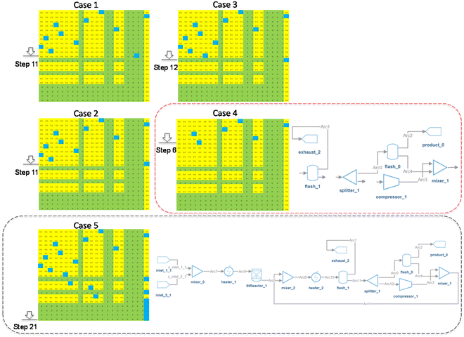Fig. 8 Five kinds of actions. Case 1: ‘inactive’ action; Case 2: ‘no action’ with ‘active’ options; Case 3: ‘no action’ without ‘active’ options; Case 4: ‘active’ action; Case 5: episode end action.

Case 1: the agent takes an “inactive” action. Anytime the AI agent steps on an “inactive” spot (the blue spot in row 11), the action will be assigned the minimum reward plus a penalty (e.g., −1000 plus −400).

Case 2: the agent takes a “no action” action when “active” spots are in the row. In this case, the action will inherit the reward of the last action (R_last) plus a penalty (e.g., −400). Please note that the penalty value is adjustable and impacts the system design complexity.

Case 3: the agent takes a “no action” action if there is no other available “active” spot in this row. In this case, the action will inherit the reward of the last action with no penalty.

Case 4: the agent takes an “active” action. In this case, the incomplete flowsheet at Step 6 (shown in the red dotted line) will be evaluated by the fast pre-screens. The reward is initialized at the beginning of the fast pre-screens with a value of 500. As the incomplete flowsheet violates Constraints 3, 5, 8, and 10, the initialized reward (500) plus the accumulated penalty (e.g., −700) will be the final deducted reward (e.g., −200).

Case 5: at the end of each iteration or episode, if the complete flowsheet satisfies all the physics constraints pre-screens, it will be sent to IDAES for re-evaluation. As seen in the black dotted line of Fig. 8, the flowsheet can be solved by IDAES, and has a feasible solution with a benzene purity of 75% and flowrate of 0.225 mol s⁻¹. In this example, the reward will be 5000 plus an extra reward associated with the benzene purity and flow rate.

3.1.2 RL-IDAES optimization results for the HDA system. The RL-IDAES framework is utilized for the conceptual design of the HDA system with different CPPs. The CPPs are listed in Table 1, each containing 14 to 20 units in the pool. The AI agent attempted to build the flowsheets with 1 million episodes for each CPP. The hyper-parameters in this proposed RL model are referenced from the pioneers' RL approach,^33,35 with further adjustments for this energy and chemical system design application. The “greedy factor ε”, “learning rate α” and “decay factor γ” are set with 0.0–0.9, 0.01 and 0.5, respectively. The “memory” size is 20 000 observations/flowsheets, and the “training batch” size is 3200.

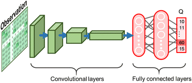
The Deep Q Network includes four convolutional layers between the observation and the fully connected layers. The convolutional neural network plays a part in structure compression, which can be turned on or off. It has been observed that CNN helps the AI agent find more feasible designs, especially for large-size CPPs, with reasonable extra computing costs. For the subsequent studies, “CNN structure compression” is always turned on. “System complexity” is controlled by the “no action” penalty. It can vary from 1 to 4 with four discrete “no action” penalties. In this section, “system complexity” is set at the highest level as the authors want the RL to involves as many units in the design as possible.

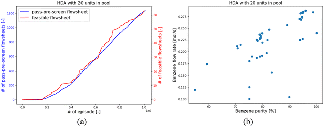
Seven RL-HDA training cases have been implemented with seven different CPPs. For each CPP, the RL agent can train from “zero” without loading any pre-trained model, and all the parameters in DQN are randomly initialized. The results are shown in Fig. 9, most of which take no more than 20 hours on a personal desktop. In Fig. 9(a), it shows the RL found thousands of unique designs passing the pre-screen process, which means they satisfy all the fundamental physics constraints. Deep blue bars “start from 0” denote RL results trained from “zero”, and light blue bars “restore HDA-20” represent RL results trained by loading a pre-trained model with 20 process-units available in CPP, which will be discussed in Section 3.2.2. Fig. 9(b) shows the number of unique feasible flowsheets found with each CPP. Orange bars “start from 0” denote RL results trained from “zero”, and yellow bars “restore HDA-20” are for RL results trained by restoring the pre-trained model, which will be discussed in Section 3.2.2.

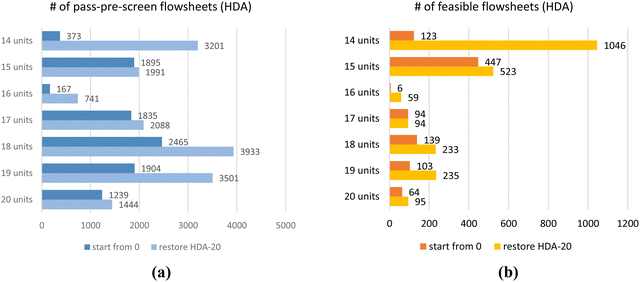Fig. 9 RL results for HDA system with different CPPs. (a) the number of flowsheets passing pre-screen; (b) the number of feasible flowsheets.

For example, with 14 units in the CPP, the “start from zero” RL found 373 unique flowsheets passing the pre-screen process, and 123 are feasible. The feasible/pass-pre-screen ratio is about 1/3. As the AI agent is highly encouraged to use all the units in the pool, certain large-size CPPs (e.g., 16 units in Fig. 9) may confuse the RL framework and may need more training to learn the strategies of building feasible flowsheets.

Taking HDA-20 as an example, the RL found 1239 pass-pre-screen flowsheets and 64 feasible ones. Fig. 10(a) shows the number of pass-pre-screen flowsheets found in the training process as the blue line and the number of feasible ones as the red line. In the first 200 000 episodes, the RL struggled to pass the pre-screen process. After that, it gradually found more and more unique feasible designs. Most of the flowsheets were found to involve 18 or 19 units in the designs.

Fig. 10 RL results for HDA system with 20 units in pool. (a) the number of flowsheets founds within 1 million episodes; (b) the benzene flow rate and Benzene purity of the 64 feasible flowsheets for HDA-20.

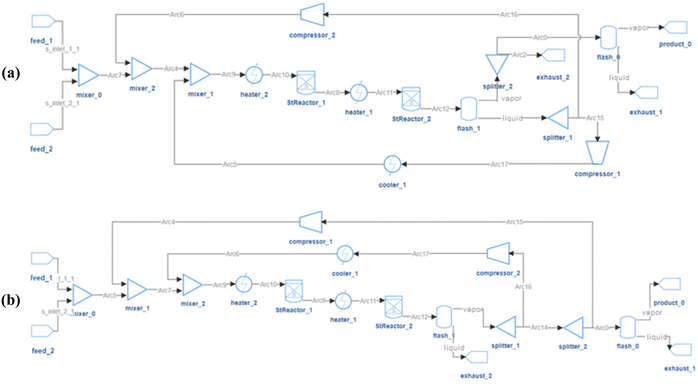
The design objective is to obtain high product-flow-rate and product-purity HDA systems, and the performances of the 64 feasible flowsheets are shown in Fig. 10(b). With the system feed of 0.3 mol s⁻¹ toluene, the product flow rate has a theoretical upper limit of 0.3 mol s⁻¹. In the 64 feasible system designs, as shown in Fig. 10(b), the highest purity is 99%, and the highest Benzene flow rate that RL designed is 0.288 mol s⁻¹. The corresponding highest-purity and highest-flow-rate designs are shown in Fig. 11(a) and (b), respectively. The flowsheet in Fig. 11(a) keeps a high volume of Benzene recirculating in the loops to increase the efficiency of the flash drum and stoichiometric reactor to obtain a high-purity product. The second design in Fig. 11(b) recycles the vapor outlet of “flash_1” to increase the utilization of system feed to achieve a high product flow rate. Notably, the core process of the second design correlates with the configuration reported in the literature as the best configuration.³⁷ It is noticed that there are some unnecessary connections in the designs, or certain designs may be unpractical. One reason is that the RL agent is encouraged to use as many process-units as possible. For HDA-20, certain units may be connected to the system but not influence the system's operation. Another reason is in this HDA demonstration case, only product flow rate and purity were considered in the system optimization target; other practical factors, such as capital cost and annualized revenue, were not counted in the designing objective. The RL-IDAES allows the user to customize the design objective. As more practical considerations are added to the IDAES optimization and the action-reward system, the RL agent will behave closer to experienced engineers.

Fig. 11 Optimal flowsheets for HDA system with 20 units in pool. (a) product purity = 99.9%, product flow rate = 0.240 mol s⁻¹; (b) product purity = 95.9%, product flow rate = 0.288 mol s⁻¹.

3.2 Methanol synthesis system and network transferability

The RL framework is expected to design different energy and chemical systems while requiring the least knowledge from the user. In this section, the RL framework is extended to develop a methanol synthesis system. According to the following reaction, the chemical system produces methanol from syngas.^38–40

CO + 2H₂ → CH₃OH (3)

The desired chemical system has two feeds. One is 2.0 mol s⁻¹ of hydrogen at the temperature of 293.15 K and pressure of 3 000 000 Pa, and the other one is 1.0 mol s⁻¹ of carbon monoxide at the temperature of 293.15 K and pressure of 3 000 000 Pa. The objective is to maximize the methanol flow rate while minimizing the unit cost of the product, defined as the sum of amortized capital cost and operation cost divided by product volume in moles. Similar to the case of the HDA system example, the design process for the methanol synthesis system allows for upstream pretreatment to reactor conditions and downstream postprocessing for heat and product recovery.

3.2.1 RL-IDAES optimization results for the methanol synthesis system. Similar to the HDA system example, the same 22 common process-units from the IDAES are made available to the methanol synthesis system. 14 to 20 of them are selected as CPPs for the AI agent to build conceptual designs, as listed in Table 2, and named as Meth-14 to Meth-20 for short. Besides the all-units (22), Meth-14 and Meth-20 are the same as the HDA system (HDA-14 and HDA-20). The initialized flowsheet shares the same size, 21 × 22, as in Fig. 7. Depending on the user-defined CPP, the selected unit inlets/rows and outlets/columns are initialized as “active” with a value of 0.5.

Table 2 Potential candidate process-units pools for methanol demonstration

No. of units	Name	Feed	Product	Exhaust	Mixer	Compressor	Heater	Reactor	Flash	Splitter	Cooler	Expander
14	Meth -14	2	1	2	2	1	1	1	1	1	1	1
15	Meth -15	2	1	2	2	2	1	1	1	1	1	1
16	Meth -16	2	1	2	2	2	2	1	1	1	1	1
17	Meth -17	2	1	2	2	2	2	1	1	2	1	1
18	Meth -18	2	1	2	2	2	2	2	1	2	1	1
19	Meth -19	2	1	2	3	2	2	2	1	2	1	1
20	Meth -20	2	1	2	3	2	2	2	2	2	1	1
22 (All)		2	1	2	3	2	2	2	2	2	2	2

---

The RL-IDAES framework has been utilized to design methanol systems with the CPPs in Table 2. The RL takes 1 million episodes for each CPP to build the flowsheets. In each episode, the draft flowsheet will be evaluated by the pre-screens and the IDAES. The training setups are the same as that of the RL-HDA: “greedy factor ε” is increasing from 0.0 to 0.9, “learning rate α” is 0.01, “decay factor γ” is 0.5, “memory size” is 20 000 and “batch” size is 3200. For all the implemented training, “CNN structure compression” is activated and “system complexity” is set to the highest level to encourage the AI agent to connect as many process-units as possible.

Seven RL-methanol training cases have been implemented with the pre-defined CPPs. All the training was completed with 15 hours on a personal computer; the results are summarized in Fig. 12. Fig. 12(a) shows the RL found pass-pre-screen flowsheets. Deep blue bars “start from 0” denote training DQN without loading any pre-trained model, and all the parameters in the DQN are randomly initialized. Light blue bars “restore HDA-20” denote training results by restoring a DQN model, which was trained for the HDA system with 20 process-units in CPP. Fig. 12(b) shows the feasible flowsheets with different CPPs; orange and yellow bars represent training results without or with loading the pre-trained DQN model. With 14 process-units, “start from zero” RL found 363 pass-pre-screen and 90 feasible flowsheets; with 15 or 16 units, the RL can still find hundreds of pass-pre-screen flowsheets, and the feasible to pass-pre-screen ratios increase to 31% or 41%; with 17 or 18 units, the RL undertook a boost in performance, more than 700 flowsheets passing the pre-screen process and about half of them are feasible. However, with more units in the pool, the RL can rarely find feasible flowsheets. This indicates that too many units don't fit such a simple reaction system.

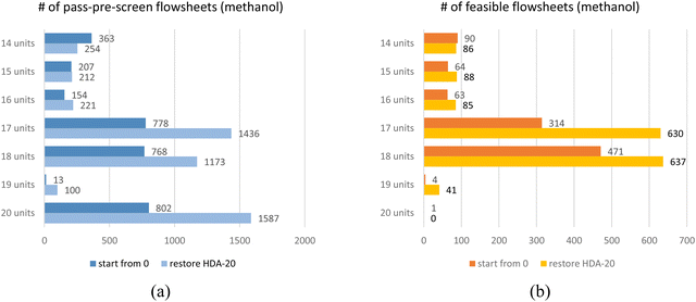Fig. 12 RL results for methanol system with different CPPs. (a) the number of flowsheets passing pre-screen; (b) the number of feasible flowsheets.

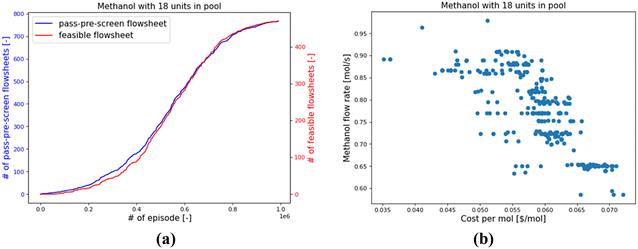
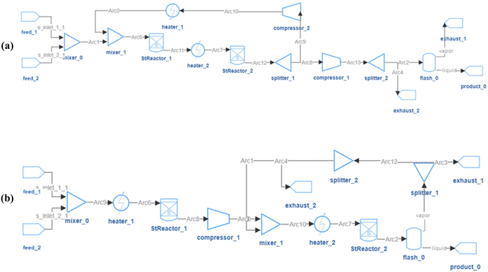
Taking the Meth-18 as an example, the RL found 768 pass-pre-screen and 471 feasible flowsheets within 1 million episodes, as shown in Fig. 13(a). Most of the feasible designs involve 15 to 17 units in the system. Their performances are shown in Fig. 13(b). The x-axis denotes the methanol's unit cost, and the y-axis represents the methanol flow rate. The costs consider the operation and amortized capital costs of certain kinds of units. As can be seen, the costs per mole of methanol range from 0.035 $ per mol to 0.072 $ per mol. Flowsheets with methanol flow rates lower than 0.55 mol s⁻¹ have been filtered as “infeasible” cases. The methanol flow rates of feasible flowsheets vary from 0.586 to 0.979 mol s⁻¹. The lowest unit-cost case is in Fig. 14(a), and the highest-flow-rate case is in Fig. 14(b).

Fig. 13 RL results for methanol system with 18 units in pool. (a) the number of flowsheets found within 1 million episodes; (b) the methanol flow rate and unit cost of the 471 feasible flowsheets for Methanol-18.

Fig. 14 Optimal flowsheets for methanol system with 18 units in pool. (a) product flow rate = 0.892 mol s⁻¹, cost per mole product = 0.035 $ per mol; (b) product flow rate = 0.979 mol s⁻¹, cost per mole product = 0.051 $ per mol.

3.2.2 DQN model transferability. The RL framework in this study intermittently saves the trained DQN model in case the training process is interrupted. The user can always continue training the model until acquiring the desired results by loading the last saved model. Except for loading the trained model with the same setup, the RL framework can also load a trained DQN model from a different CPP or even a different energy and chemical system. The RL framework has a universal observation template, and initialized flowsheets with different CPPs share the same size and structure. Available common process-units for the HDA and methanol synthesis system designs are the same. Therefore, the RL-methanol case can load a pre-trained model from the RL-HDA case. If another energy or chemical system design adopts the same observation template, trained DQN models from any of these systems can be transferred to the others. Fig. 9 and 12 show the network transferability between different CPPs and systems.

Restoring a pre-trained DQN model has proven to improve the RL's performance while reducing computing costs. As shown in light blue bars in Fig. 9(a) and yellow bars in Fig. 9(b), by restoring the DQN model trained with the 20-CPP for 1 million episodes (noted as HDA-20), all seven training cases have increased in performance. For the case with the 20-CPP, the RL found 16% more pass-pre-screen and 48% more feasible flowsheets. For the case with the 14-CPP, the RL found an 8.5 times increase in pass-pre-screen and feasible flowsheets after restoring the HDA-20 model. The RL-methanol cases for seven CPPs were retrained by restoring the same HDA-20 model as well. Results are shown in Fig. 12(a) and (b) compared to the “start from zero” results. With large-size CPPs (e.g., 17, 18 units in the pool), restoring a pre-trained model makes significant differences. For example, with 17 units in the pool, the RL found about 100% more pass-pre-screen and feasible designs. With other CPPs, one can still see some improvement in the RL's performances.

3.3 RL performance improvement by adequate training episodes

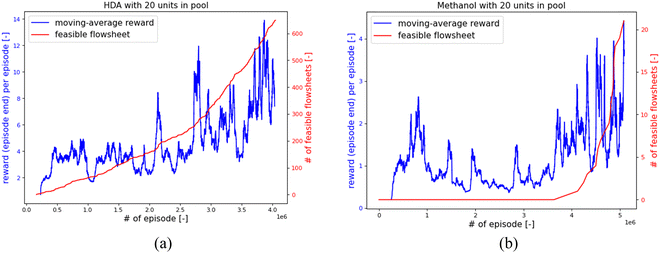
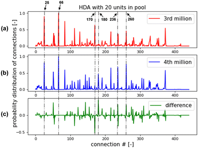
For comparing the RL performance fairly for different CPPs and chemical systems, the training episodes were limited to 1 million in the above sections. In such a situation, a few RL training cases have relatively poor performances, such as HDA-16, HDA-20, Meth-19 and Meth-20. For example, fewer pass-pre-screen or feasible flowsheets were found for HDA-16 than for HDA-15 or HDA-17. For Meth-20, the AI agent can rarely find a feasible design within 1 million episodes. This issue can be resolved by increasing the training episodes. Two example tests for HDA-20 and Meth-20 were conducted, as shown in Fig. 15. For the HDA-20 case, with “greedy factor ε” fixed at 0.9 and other set-ups kept the same, the RL training was continued for another 3 million episodes. In Fig. 15(a), the “moving averaged reward” is plotted against the training episodes as the blue line, and the number of feasible flowsheets in the training process is plotted as the red line. The “moving averaged reward” is calculated by dividing the rewards of pass-pre-screen flowsheets by the number of episodes the AI agent takes to find them. As can be seen in the plot, the moving average reward generally increases in the continuing 3 million ‘episodes’ training. At the same time, the number of feasible flowsheets rises faster as the training goes on. The Methanol-20 case continued training for another 5 million with “greedy factor ε” is fixed at 0.9; the results are shown in Fig. 15(b). One can see that, in the first 4 million episodes, the RL is struggling to explore the strategies to build flowsheets. But at the 5th million episodes, it finds the right way to construct feasible flowsheets. Also, the moving average reward keeps a generally increasing trend, and the number of feasible flowsheets keeps rising.

Fig. 15 RL performance as training continuing, blue line denoting reward per episode, red line representing number of feasible flowsheets. (a) for HDA system with 20 units in pool. (b) for methanol system with 20 units in pool.

In order to explore the mechanism behind the training performance improvement, the RL found feasible flowsheets are analyzed. As presented in Section 3.1, the HDA or methanol system is denoted by a 21 × 21 matrix. And the matrix contains 441 potential connections. Counting the appearances of each connection in the RL found flowsheets, the probability distribution of each connection can be obtained. The probability distribution function (PDF) of connections for the HDA-20 is shown in Fig. 16. The PDF of connections for the feasible flowsheets found within the 3rd million is shown in Fig. 16(a), the PDF of connections for the feasible flowsheets found in the 4th million is shown in Fig. 16(b), and their difference is shown in Fig. 16(c). As marked in Fig. 16(a) and (b) share several peaks, such as at Connection 66. Connection 66 denotes “flash_0's vapor outlet connects to product_0's inlet”. It means the AI agent thought this connection was necessary for a feasible flowsheet early in the 3rd million episodes. Comparing Fig. 16(a) and (b), one can see that the peak at Connection 170 in Fig. 16(a) diminishes in Fig. 16(b), while new peaks at Connections 180, 236, and 260 appear in Fig. 16(b). This indicates in the 4th million episodes' training, and the RL learned to break the connection from mixer_2 to heater_1, then build a chain of connections “splitter_1 to heater_1, to StReactor_2, and to flash_1”. Learning these changes should help the AI agent to find more feasible designs.

Fig. 16 Probability distribution function of connections for HDA system with 20 units in pool. (a) for feasible flowsheets found within the 3^rd million of episodes; (b) for feasible flowsheets found within the 4^th million of episodes; (c) Difference between (b) and (a).

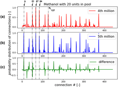
The RL-methanol case experiences a significant improvement in the 5th million episodes. The probability distribution functions (PDFs) of connections for RL found flowsheets in 4th million episodes and 5th million episodes are shown in Fig. 17(a) and (b), respectively. Their difference is shown in Fig. 17(c). The RL has learned to build several essential connections in the early stage, such as Connection 67, “flash_0's liquid outlet connecting to product_0's inlet”. Both Fig. 17(a) and (b) peak at this connection. PDFs for the 5th million episodes in Fig. 17(b) have stronger peaks than that of the 4th million episodes in Fig. 17(a) at Connection 84 and 127. These two connections denote that mixer_0 integrates with mixer_1 and mixer_2 to be a four-inlet mixer. It will ensure recycling loops go upstream of the system. What makes a dramatic change in the 5th million episodes is that the RL breaks Connection 51 and builds Connection 9, which means it connects flash_1's liquid outlet to flash_0's inlet instead of exhaust_2's inlet. In other words, the methanol stream in flash_1's liquid outlet can go to flash_0 and then product_0 instead of exhausting the system.

Fig. 17 Probability distribution function of connections for methanol system with 20 units in pool. (a) for feasible flowsheets found within the 4^th million of episodes; (b) for feasible flowsheets found within the 5^th million of episodes; (c) Difference between (b) and (a).

4. Conclusion

Traditional computer-aided process engineering and conceptual design of energy and chemical systems require lots of expert human mediation, either providing the initially drafted flowsheet and/or alternative connections. Typically, selecting and evaluating feasible system designs relies on the engineer's knowledge and experiences. This study proposes a more flexible reinforcement learning-based automated approach for the conceptual design of energy and chemical processes and automatically interacting with a general energy system modeling platform, IDAES. It requests the least knowledge from the user for solving the conceptual design problem applied to energy and chemical systems. The IDAES module library provides all the available energy and chemical process units and corresponding operations (e.g., phase change, temperature change, pressure change, etc.) that are allowed to be used in the system. The AI agent automatically selects units from the user-defined CPPs, connects them to construct flowsheets, and optimizes the system design according to the user's desired objective. The AI agent does not need any integrated pre-defined rule about the system design. The AI agent only learns from the reward scores provided by the IDAES simulation and a fast pre-screen evaluation system.

Two demonstration case studies have been implemented. The RL-IDAES framework has been proven to design and optimize complicated hydrodealkylation of toluene and methanol synthesis systems with high flexibility at affordable computing costs. For example, 123 feasible designs for the HDA system with 14-CPP can be found within 20 hours on a PC. The RL framework can share a universal observation template among different CPPs or energy and chemical systems. A trained DQN model can be transferred to other training cases. Restoring a pre-trained DQN model has proven to improve the RL's performance. As demonstrated in Section 3.2.2, the DQN model trained for the HDA system can be directly used in methanol synthesis system design and found more feasible designs with limited training episodes. In some cases, the RL framework may struggle to learn the strategies for building feasible flowsheets within the limited 1 million training episodes, especially for cases with relatively large CPPs. However, as demonstrated in Section 3.3, with adequate training episodes, the AI agent can eventually discover the key connections in the system and discard the distracting connections, significantly increasing the number of feasible designs.

Data and code availability

The RL framework code and the two example systems are open-source available at https://github.com/pnnl/RL-Energy. The source code for the Institute for the Design of Advanced Energy Systems is open-source available at https://idaes.org/.

Nomenclature

1D	1-Dimensional
AI	Artificial intelligence
C	Compressor
CNN	Convolutional neural network
CPP	Candidate process-units pool
DNN	Deep neural network
DOE	Department of Energy
DQN	Deep Q value network
F	Feed
FL	Flash
γ	Decay factor
H	Heater
HDA	Hydrodealkylation reaction
IDAES	Institute for the design of advanced energy system
M	Mixer
ML	Machine learning
NETL	National energy technological laboratory
P	Product
Q	Q Value
Q next	Future Q values
R	Reactor, reward
RL	Reinforcement learning
Rlast	Reward of the last action
RL-IDAES	RL-Guided energy and chemical systems design framework
RMSProp	Root mean squared propagation

Conflicts of interest

There are no conflicts to declare.

Acknowledgements

The authors would like to acknowledge the financial support from the U.S. Department of Energy's Advanced Research Projects Agency-Energy (ARPA-E) Design Intelligence Fostering Formidable Energy Reduction and Enabling Novel Totally Impactful Advanced Technology Enhancements (DIFFERENTIATE) program under project 19/CJ000/09/01. Computational resources were provided by Pacific Northwest National Laboratory (PNNL) Research Computing. PNNL is a multi-program national laboratory operated for the U.S. Department of Energy by Battelle under Contract DOE-AC05-76RL01830. The authors would like to acknowledge David Millar and Anthony P. Burgard in the National Energy Technology Laboratory for their advice on technical works and project management. National Energy Technology Laboratory (NETL) Disclaimer: This project was funded by the United States Department of Energy, National Energy Technology Laboratory, in part through a site support contract. Neither the United States Government nor any agency thereof, nor any of their employees, nor the support contractor, nor any of their employees, makes any warranty, express or implied, or assumes any legal liability or responsibility for the accuracy, completeness, or usefulness of any information, apparatus, product, or process disclosed, or represents that its use would not infringe privately owned rights. Reference herein to any specific commercial product, process, or service by trade name, trademark, manufacturer, or otherwise does not necessarily constitute or imply its endorsement, recommendation, or favoring by the United States Government or any agency thereof. The views and opinions of authors expressed herein do not necessarily state or reflect those of the United States Government or any agency thereof.

References

1. S. Stephanopoulos and G. V. Reklaitis, Process systems engineering: from solvay to modern bio- and nanotechnology. a history of development, successes and prostpects for the future, Chem. Eng. Sci., 2011, 66(19), 4272–4306.
2. Q. Gottl, D. G. Grimm and J. Burger, Automated synthesis of steady-state continuous processes uing reinforcemnt learning, Front. Chem. Sci. Eng., 2022, 16(2), 288–302.
3. R. W. H. Sargent and A. W. Westerberg, SPEED-UP in chemical engineering design, Trans. Inst. Chem. Eng., 1964, 42, 190–197.
4. A. I. Johnson, Computer Aided Process Analysis and Design—A Modular Approach, Br. Chem. Eng. Process Technol., 1972, 17(1), 28.
5. J. D. Seader, et al., Flotran simulation: an introduction, CACHE, Cambridge, Mass., 1977.
6. C. Chen, et al., Local composition model for excess Gibbs energy of electrolyte systems. Part I: single solvent, single completely dissociated electrolyte systems, AIChE J., 1982, 28(4), 588–596.
7. I. E. Grossmann and I. Harjunkoski, Process Systems Engineering: Academic and industrial perspectives, Comput. Chem. Eng., 2019, 126, 474–484.
8. J. J. Siirola, Strategic process synthesis: advances in the hierarchical approach, Comput. Chem. Eng., 1996, 20(S2), S1637–S1643.
9. R. W. H. Sargent and K. Gaminibandara, Optimum desing of plate distrillation columns, in Optimization in Action, ed. L. C. W. Dixon, 1976, Academic Press, London, pp. 267–314.
10. Q. Chen and I. E. Grossmann, RRecent developments and challenges in optimization-based process synthesis, Ann. Rev. Chem. Biomol. Eng., 2017, 8(1), 249–283.
11. H. Yeomans and I. E. Grossmann, A systematic modeling framework of superstrucure optimization in process synthesis, Comput. Chem. Eng., 1999, 23(6), 709–731.
12. G. Stephanopoulos and A. W. Westerberg, Studies in process synthesis II, evolutionary synthesis of optimal process flowsheets, Chem. Eng. Sci., 1976, 31(3), 195–204.
13. T. Zhang, N. V. Sahinidis and J. J. Siirola, Pattern recognition in chemical process flowsheets, AIChE J. Am. Instit. Chem. Eng., 2019, 65(2), 592–603.
14. G. Montavon, W. Samek and K. Muller, Methods for interpreting and understanding deep neural networks, Digital Signal Process., 2018, 73, 1–15.
15. D. Wang, et al., Machine Learning Tools Set for Natural Gas Fuel Cell System Design, ECS Trans., 2021, 103(1), 2283–2292.
16. I. J. Goodfellow, et al., Generative Adversarial Nets, arXiv, 2014.
17. A. Radford, L. Metz and S. Chintala, UNSUPERVISED REPRESENTATION LEARNINGWITH DEEP CONVOLUTIONAL GENERATIVE ADVERSARIAL NETWORKS. arXiv, 2016.
18. A. Sciazko, Y. Komatsu and N. Shikazono, Unsupervised Generative Adversarial Network for 3-D Microstructure Synthesis from 2-D Image, Electrochem. Soc. Trans., 2021, 103(1), 1363–1373.
19. B. Mildenhall, et al., NeRF: Representing Scenes as Neural Radiance Fields for View Synthesis. arXiv:2003.08934, 2020.
20. A. Vaswani, et al., Attention is all you need, in 31st Conference on Neural Information Processing Systems. 2017: Long Beach, CA, USA.
21. L. P. Kaelbling, M. L. Littman and A. W. Moore, Reinforcement learning: a survey, J. Artificial Intelligence Res., 1996, 4, 237–285.
22. D. Silver, et al., Mastering the game of Go with deep neural networks and tree search, Nature, 2016, 529, 484–489.
23. B. J. Pandian and M. M. Noel, Control of a bioreactor using a new partially supervised reinforcement learning algorithm, J. Process Control, 2018, 69, 16–29.
24. A. A. Khan and A. A. Lapkin, Designing the process designer: Hierarchical reinforcement learning for optimisation-based process design, Chem. Eng. Process., 2022, 180, 108885.
25. A. Khan and A. Lapkin, Searching for optimal process routes: a reinforcement learning approach, Comput. Chem. Eng., 2020, 141, 107027.
26. Q. Göttl, D. G. Grimm and J. Burger, Using Reinforcement Learning in a Game-like Setup for Automated Process Synthesis without Prior Process Knowledge, Computer Aided Chemical Engineering, Elsevier, 2022, pp. 1555–1560.
27. Q. Göttl, D. G. Grimm and J. Burger, Automated synthesis of steady-state continuous processes using reinforcement learning, Front. Chem. Sci. Eng., 2022, 1–15.
28. Q. Göttl, et al., Automated flowsheet synthesis using hierarchical reinforcement learning: proof of concept, Chem. Ing. Tech., 2021, 93(12), 2010–2018.
29. A. Lee, et al., The IDAES process modeling framework and model library—Flexibility for process simulation and optimization, J. Adv. Manuf. Process., 2021, 3(3), e10095.
30. National Energy Technology Laboratory, e.a. Read the Docs: Institute for the Design of Advanced Energy Systems (IDAES). 2016-2021 [cited 2022]; stable:[Available from]: https://idaes-pse.readthedocs.io/en/stable/.
31. National Energy Technology Laboratory, e.a. GitHub: IDAES Toolkit. 2022 [cited 2022]; 2.0.0a0:[Available from]: https://github.com/IDAES/idaes-pse.
32. W. E. Hart, et al., Pyomo-optimization modeling in python, Springer, 2017, vol. 67.
33. A. Wächter and L. T. Biegler, On the implementation of an interior-point filter line-search algorithm for large-scale nonlinear programming, Math. Prog., 2006, 106(1), 25–57.
34. M. Abadi et al. TensorFlow: A system for large-scale machine learning, in Software available from tensorflow.org. 2016.
35. G. Hinton, N. Srivastava and K. Swersky, Neural networks for machiine learning, Overview of mini-batch gradient descent. 2012.
36. R. Turton, et al., Analysis, Synthesis, and Design of Chemical Processes, Pearson College Div, 3rd edn, 2008.
37. J. M. Douglas, Chemical Design of Chemical Processes, McGraw-Hill, 1988.
38. L. G. A. V. D. Water, et al., Understanding methanol synthesis from CO/H₂ feeds over Cu/CeO₂ catalysts, J. Catal., 2018, 364, 57–68.
39. I. A. Fisher and A. T. Bell, In Situ Infrared Study of Methanol Synthesis from H₂/CO over Cu/SiO₂ and Cu/ZrO₂/SiO₂, J. Catal., 1998, 178, 153–173.
40. G. J. J. Bartley and R. Burch, Support and morphological effects in the synthesis of methanol over Cu/ZnO, Cu/ZrO₂ and Cu/SiO₂ catalysis, Appl. Catal., 1988, 43, 141–153.

---