 Open Access Article
Creative Commons Attribution 3.0 Unported Licence
Perspectives for analyzing non-linear photo-ionization spectra with deep neural networks trained with synthetic Hamilton matrices
Sajal Kumar
Giri
*,
Lazaro
Alonso
*,
Ulf
Saalmann
 * and
Jan Michael
Rost
 *
*
Max Planck Institute for the Physics of Complex Systems, Nöthnitzer Str. 38, Dresden, 01187, Germany. E-mail: sajal@pks.mpg.de; lalonso@pks.mpg.de; us@pks.mpg.de; rost@pks.mpg.de
First published on 15th December 2020
Abstract
We have constructed deep neural networks, which can map fluctuating photo-electron spectra obtained from noisy pulses to spectra from noise-free pulses. The network is trained on spectra from noisy pulses in combination with random Hamilton matrices, representing systems which could exist but do not necessarily exist. In [Giri et al., Phys. Rev. Lett., 2020, 124, 113201] we performed a purification of fluctuating spectra, that is, mapping them to those from Fourier-limited Gaussian pulses. Here, we investigate the performance of such neural-network-based maps for predicting spectra of double pulses, pulses with a chirp and even partially-coherent pulses from fluctuating spectra generated by noisy pulses. Secondly, we demonstrate that along with purification of a fluctuating double-pulse spectrum, one can estimate the time-delay of the underlying double pulse, an attractive feature for single-shot spectra from SASE FELs. We demonstrate our approach with resonant two-photon ionization, a non-linear process, sensitive to details of the laser pulse.
1 Introduction
Machine learning (ML) has recently been applied not only in physics,1–3 but more specifically in strong-field physics.4–6 One of the most abundant topics has been the reconstruction of the temporal shape of an ultrashort laser pulse, aided by ML techniques.7–9 The most popular techniques for this reconstruction have been different variants of streaking techniques which normally require considerable additional experimental effort, namely a Terahertz laser light source. With its help, one can generate a large amount of data—the streaking traces—which can be processed with ML to extract the attosecond pulse shape.7,8 However, also a direct method from single-shot spectra has been introduced.9In a different vein, a trained neural network has been proposed to represent a (semi-)classical path integral for strong-field physics,10 replacing the need to explicitly calculate a large number of classical trajectories to eventually determine the photo-ionization cross section, which is, however, still an approximation as it is constructed semi-classically. To supply training data for a network which can represent the full quantum path integral, implies most likely use of a numerical effort that would be higher than calculating observables directly.
In general, training of a deep neural network needs a very large amount of non-trivial training data. To generate them experimentally requires substantial additional effort (see the streaking example above). To obtain such data without serious approximations within theory is often prohibitively expensive, as in the second example.
Acknowledging this situation, we have invented another approach: to calculate exactly and explicitly (with the time-dependent Schrödinger equation) photo-electron spectra with a large number of pulses and artificial systems, for which the calculation can be done very quickly. In this way we are able to supply learning data consisting of about 107 spectra. A network trained with these synthetic systems, is not only able to purify noisy test spectra unknown to the network, but from the same class of synthetic systems the training was performed with. Also “real” spectra can be purified, which could come from experiment, or for this work, from a realistic full calculation with parameters for the helium atom. Moreover, noise is, in the context of machine learning, helpful when applied to non-linear photo-ionization: photo-excitation and ionization processes are subject to strict angular-momentum selection rules, thereby limiting the coupling of light to matter. If a light pulse contains noise and operates in a non-linear (at least two-photon absorption) regime it will couple to a much larger part of the electron dynamics of the target. This helps to train the mapping better and enlarges the pool of training spectra naturally.
In general, all trained networks we will present, map one type of spectrum into another (desired) one for a photo-ionization scenario of which only a few key elements need to be specified: the target system should have an excited state around the photon energy ω*, above the ground state, and intensities of the light pulse should be such that two-photon processes dominate. It is not necessary to know more about the target system, as ideally all target systems accessible by the light as specified are covered by the learning space for the synthetic systems, represented by synthetic Hamilton matrices (SHMs). Therefore, one can apply a trained network also to an experimental spectrum from noisy pulses without detailed knowledge of the target system.
Once the design for training such networks with SHMs is set up, that is, the spectra for learning have been computed, it is not difficult to construct other maps with new networks, as the major effort is to supply the learning data which do not have to be changed, while training new networks is computationally relatively cheap. This allows us to provide several mappings in the following to predict spectra for ideal double, chirped and even highly structured partially coherent pulses from noisy spectra. Finally, we will introduce network based mapping for a typical SASE FEL situation: there, single-shot noisy spectra are recorded which depend on further, not explicitly known parameters, e.g., the geometrical orientation of the sample or the time-delay of double pulses used. Considering the latter situation, we reconstruct from noisy spectra simultaneously the noise-free spectra and the time-delay of the double pulse. While we cannot do this with the accuracy of the designated algorithms as described in the context of streaking above, we do not need any additional information but the spectrum itself.
The paper is organized as follows: in Section 2 we give details on the representation of the noisy pulses, explain how to construct the SHMs and describe our fast propagation scheme to solve the electronic Schrödinger equation to obtain the photo-ionization spectra. Section 3 details how the network is trained and set up, including measures on how to quantify errors in the reconstruction of spectra and a convenient way to parameterize them. In Section 4 we present the predictions of the photo-ionization spectra for various pulse forms. Section 5 discusses the single-shot FEL scenario. The paper ends with conclusions in Section 6.
2 Prerequisites
To determine the photo-ionization dynamics we need two elements, the noisy pulses and an efficient way to describe the electron dynamics. In the end we will specify the process we are interested in, namely two-photon absorption.2.1 Pulses
We distinguish between the “noisy pulses” which lead to fluctuating spectra and the “reference pulses” for which we want to predict spectra.There are many different possibilities for incorporating noise into a signal. We choose the partial-coherence method.11,12 With this method one can create noisy pulses whose average over an ensemble has a well-defined pulse shape. As experimentally demonstrated,12 these kinds of pulses represent pulses from SASE FELs well. In the following, we will use the pulse parameterisation
| f(t) = NGT(t)Fτ(t), | (1a) |
 | (1b) |
 and
and  are the Fourier transform and its inverse, and ω* is the carrier frequency. Noise is introduced through random spectral phases ϕ, uniformly distributed in the interval −π ≤ ϕ ≤ +π. The time scale of the fluctuations is given by the coherence time τ, while the Gaussian GT(t) limits the typical pulse duration to T. Otherwise, the pulse duration could grow beyond all limits due to the presence of random spectral phases. A specific (deterministic) noise realization we will label with ϕl(ω). If not stated otherwise, we use T = 3 fs and τ = 0.5 fs in the following. In order to deal with comparable pulses, we use the normalisation constant N to fix the pulse energy Ep, which would otherwise fluctuate from realisation to realisation.
Any reasonable pulse can serve as a reference pulse, for which the map created by the network can predict the spectrum. Reasonable means in the present context that the reference pulse’s frequency spectrum is covered by the learning space of fluctuating spectra. The simplest choice is the Gaussian GT(t) in eqn (1) itself rendering the prediction equivalent to removing the fluctuations from the spectrum. Therefore, we call this type of map “purification”.6 In Section 5 we will purify fluctuating spectra from double pulses.
2.2 Paradigmatic 1-dimensional strong-field electron dynamics
Although the subsequent scheme to construct SHMs is general, for the sake of clarity we will describe it for the processes we will consider as an example, namely two-photon absorption in a helium atom. Thereby, the carrier frequency ω* of the laser is chosen to be quasi-resonant with the transition energy to the first optically allowed excited state.A simple and convenient way to realize this concept is to consider 1D dynamics with a soft-core potential. The corresponding active one-electron Hamiltonian for helium is given by
 | (2) |
 which gives a ground-state energy E0 = −24.2 eV, close to the ionization potential of real helium (24.6 eV). We represent the Hamiltonian on a grid xj = jΔx, with Δx = 0.067 a.u. and xmax = 500 a.u., and determine by diagonalization the eigenenergies H0|α〉 = |α〉Ẽα, from the ground state up to Ẽα ≤ Emax ≈ 48 eV, resulting in 600 eigenstates.
With these eigenstates we calculate the matrix of the time-dependent Hamiltonian H(t) = H0 + A(t)![[p with combining circumflex]](https://www.rsc.org/images/entities/i_char_0070_0302.gif) in velocity gauge
in velocity gauge
 | (3) |
2.3 Synthetic Hamilton matrices (SHMs)
Since we want to train our network such that it recognizes almost arbitrary systems, which only need to have a (quasi-)resonant transition energy for the first absorbed photon, we create SHMs by randomly changing energies Eα, and matrix elements Vαβ, about the 1D example system defined in eqn (2) and (3) through the variation of four parameters in| Eα = 3[ξ1−γ]Ẽα for Ẽα < 0, α > 0, | (4a) |
| V0α = 3ξ2Ṽ0α for Ẽα < 0, | (4b) |
| Vαβ = 3ξ3Ṽαβ for Ẽα < 0, Ẽβ > 0, | (4c) |
| Vαβ = 3ξ4Ṽαβ for Ẽα > 0,Ẽβ > 0. | (4d) |
The idea of SHM is an essential part of our approach which serves two purposes: (i) it allows us to supply a sufficient number of theoretical learning data for the network and (ii) it represents a large variety of systems which could exist in nature but do not necessarily. The SHM should be “dense enough” in the parameter space such that always the Hamilton matrix of a real system one is interested in can be interpolated between SHMs, as interpolation capability is a strength of neural networks (in contrast to extrapolation). Of course, one can formulate more sophisticated SHMs with more parameters, but for the present case the four random parameters are sufficient.
Yet, we need to overcome one final obstacle, and that is the calculation of the spectra based on the SHMs. To obtain those spectra for arbitrary pulse forms A(t) requires us to solve the time-dependent Schrödinger equation (TDSE) which in turn implies that we need an extremely fast propagation scheme to be able to solve the order of 107 TDSEs in a reasonable time.
2.4 Fast solution of the TDSE with SHMs
To achieve high propagation efficiency, we make use of the fact that the Hamilton matrix eqn (3) depends explicitly on time only through the vector potential A = A(t). Hence, instead of discretizing the time equidistantly, we discretize the vector potential Amin ≤ A ≤ Amax in jmax, steps with Aj = jδA with δ A = (Amax − Amin)/(jmax − 1).With the time-independent Hamiltonian Hj = H0 + Aj![[thin space (1/6-em)]](https://www.rsc.org/images/entities/char_2009.gif)
![[p with combining circumflex]](https://www.rsc.org/images/entities/i_char_0070_0302.gif) , we can construct a short-time propagator which is valid over a time span δtj short enough such that a fixed Aj is a reasonable approximation. Therefore, the unitary short-time propagator can be obtained by direct integration,
, we can construct a short-time propagator which is valid over a time span δtj short enough such that a fixed Aj is a reasonable approximation. Therefore, the unitary short-time propagator can be obtained by direct integration,
| Uj = e−iHjδtj. | (5) |
The full propagator  , is now simply a concatenation of the short-time propagators over respective time spans δtk (with k = 1, …, kmax) over which the discretized Aj hold, where δt1 = t1 − ti and δtkmax = tf − tkmax−1.
To make efficient use of the SHMs, it is imperative that we use the matrix elements from eqn (4) as they do not require explicit integration over wave functions. Hence, we diagonalize 〈α|Hj|β〉 = Eαδαβ + jδAVαβ in the basis of H0 to give its eigenenergies Ejγ and eigenfunctions  leading to the short-time propagator
 | (6) |
Note, that over the entire pulse A(t) certain Aj may occur more than once with different time intervals over which they are valid (if the local derivative dA(t)/dt|Aj is large, the time interval will be small and vice versa). Therefore it is worthwhile to compute the Ujαβ beforehand and keep them stored. They can be used for all pulses (the fluctuating ones as well as the reference one) for a Hamilton matrix specified by the elements in eqn (4). Furthermore, we do not calculate the full matrix of the propagator which would involve many matrix products. It is sufficient to propagate the vector |0〉 of the initial state (the ground state of the system) which requires only the computation of matrix-vector products. Only in this way were we able to calculate the millions of spectra, necessary to train the network.
3 Training the network
Through training with fluctuating spectra from the SHMs, the deep neural network encodes the dynamics of two-photon absorption spectra with the central photon frequency ω* for all target systems covered by the SHMs. If the network “sees” during training a specific class of spectra much more often than representatives of other classes, it will be biased towards those often found spectra once trained. Hence, we have to fill the learning space of spectra (available for training, validating and testing the network) as homogeneously as possible.3.1 Generating spectra
Synthetic Hamilton matrices which nearly satisfy the resonance condition, i.e., ξ1 = 0 in eqn (4), are particularly sensitive to the pulse shape and therefore generate more structured and diverse spectra through nonlinear processes, here resonant two-photon ionization, than SHMs with ξ1 ≠ 0. To sample the space of input spectra as homogeneously as possible, 50% of the spectra come from SHMs with ξ1 ≈ 0 and the other 50% of spectra are from SHMs with uniform ξ1, randomly selected in the range [−1, +1]. After training on these spectra the network is not biased for ξ1 around zero but works equally well for all ξ1 in the specified range.We calculate nmat = 40![[thin space (1/6-em)]](https://www.rsc.org/images/entities/char_2009.gif) 000 reference spectra from the same number of SHMs. For each reference spectrum, we calculate npul = 200 spectra (“fluctuating spectra”) from noisy pulses obtained with the partial-coherence method11 using a different noise realization for each SHM. Since solving the TDSE for a single spectrum takes only a few seconds thanks to the highly-optimized propagation scheme outlined in Section 2.4, this procedure can be executed despite the need to solve about 107 TDSEs.
000 reference spectra from the same number of SHMs. For each reference spectrum, we calculate npul = 200 spectra (“fluctuating spectra”) from noisy pulses obtained with the partial-coherence method11 using a different noise realization for each SHM. Since solving the TDSE for a single spectrum takes only a few seconds thanks to the highly-optimized propagation scheme outlined in Section 2.4, this procedure can be executed despite the need to solve about 107 TDSEs.
For each SHM, we average over all fluctuating spectra  instead of using the individual fluctuating spectra Pkl(E) computed from Hkl(t), where k labels the Hamilton matrix and l the noisy pulse. We normalize all averaged fluctuating and reference spectra, i.e.,
  .
.
The resulting set of 40![[thin space (1/6-em)]](https://www.rsc.org/images/entities/char_2009.gif) 000 averaged fluctuating spectra constitutes a major part of the learning space to train the networks in Section 4 for the prediction of spectra from different pulse shapes.
000 averaged fluctuating spectra constitutes a major part of the learning space to train the networks in Section 4 for the prediction of spectra from different pulse shapes.
3.2 Parameterization of spectra and cost functions
For efficient representation we parameterize each spectrum![[P with combining macron]](https://www.rsc.org/images/entities/i_char_0050_0304.gif) k(E) in a basis of harmonic oscillator eigenfunctions {χκ},
k(E) in a basis of harmonic oscillator eigenfunctions {χκ}, | (7) |
![[C with combining macron]](https://www.rsc.org/images/entities/b_char_0043_0304.gif) ≡ {
≡ {![[C with combining macron]](https://www.rsc.org/images/entities/i_char_0043_0304.gif) 1…
1…![[C with combining macron]](https://www.rsc.org/images/entities/i_char_0043_0304.gif) nbas} of coefficients. A basis size of nbas = 100 is required for the averaged fluctuating spectra, while for the noise-free spectra nbas = 60 is sufficient.
nbas} of coefficients. A basis size of nbas = 100 is required for the averaged fluctuating spectra, while for the noise-free spectra nbas = 60 is sufficient.
The network maps the coefficients of the fluctuating spectra to those of the predicted underlying noise-free spectrum, {![[C with combining macron]](https://www.rsc.org/images/entities/b_char_0043_0304.gif) k} → {Ck}. The goal of the training is to minimize the difference between the predicted vector Ck for the noise-free spectrum and Crefk of the expected reference spectrum. The coefficients allow us to define a difference familiar from vector spaces as
k} → {Ck}. The goal of the training is to minimize the difference between the predicted vector Ck for the noise-free spectrum and Crefk of the expected reference spectrum. The coefficients allow us to define a difference familiar from vector spaces as
 | (8a) |
 | (8b) |
 | (8c) |
 | (8d) |
3.3 The training setup
The full set of learning data contains nmat = 40![[thin space (1/6-em)]](https://www.rsc.org/images/entities/char_2009.gif) 000 pairs of spectra. Each pair consists of an averaged noisy spectrum with its respective reference spectrum for the same SHM. The full learning data set with nmat pairs is split into training (80%), validation (10%) and test (10%) data. Training corresponds mathematically to minimizing the cost function eqn (8a), with Ω = train. Fig. 1 provides a sketch of what goes into training and prediction.
000 pairs of spectra. Each pair consists of an averaged noisy spectrum with its respective reference spectrum for the same SHM. The full learning data set with nmat pairs is split into training (80%), validation (10%) and test (10%) data. Training corresponds mathematically to minimizing the cost function eqn (8a), with Ω = train. Fig. 1 provides a sketch of what goes into training and prediction.
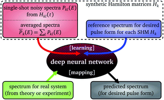 | ||
| Fig. 1 Sketch of training and use of a deep neural network with synthetic Hamilton matrices and noisy spectra. | ||
Implemented with the deep-learning library KERAS,13 a fully connected feed-forward artificial neural network is used to establish the mapping. It contains 5 layers with 60 neurons on each and was trained at a learning rate of 0.001 with 100 epochs, a batch size of 200 and a learning patience of 25. Each hidden layer neuron contains a ReLU activation function.14 The Adam optimizer15 is used to minimize the cost function, eqn (8a). The training success is quantified with the error functions eqn (8a) and (8d), which both decay logarithmically with the size of the learning data, typical for deep learning.16,17
4 Prediction of spectra for different pulse shapes
To assess the quality of the mapping achieved with the trained networks on the basis of the SHM learning data, we will discuss scenarios with three different reference pulses for which we predict spectra: (i) double pulses with different time delays Td and peak amplitude ratios A1![[thin space (1/6-em)]](https://www.rsc.org/images/entities/char_2009.gif) :
:![[thin space (1/6-em)]](https://www.rsc.org/images/entities/char_2009.gif) A2, (ii) chirped pulses with chirp parameter β, and (iii) partially coherent reference pulses with different coherence times τ according to eqn (1). We have used the network setup for all three scenarios as described in the previous section with the same set of fluctuating spectra for training, but paired for each SHM with reference spectra which differ to the corresponding above reference pulses. The fluctuating spectra used as the input of the network have been generated with the pulses from eqn (1) with a pulse length of T = 3 fs, a coherence time of τ = 0.5 fs, central photon frequency of ω* = 21 eV and spectral intensities between 8 × 10¹⁵ W fs cm−2 and 8 × 10¹⁶ W fs cm−2.
A2, (ii) chirped pulses with chirp parameter β, and (iii) partially coherent reference pulses with different coherence times τ according to eqn (1). We have used the network setup for all three scenarios as described in the previous section with the same set of fluctuating spectra for training, but paired for each SHM with reference spectra which differ to the corresponding above reference pulses. The fluctuating spectra used as the input of the network have been generated with the pulses from eqn (1) with a pulse length of T = 3 fs, a coherence time of τ = 0.5 fs, central photon frequency of ω* = 21 eV and spectral intensities between 8 × 10¹⁵ W fs cm−2 and 8 × 10¹⁶ W fs cm−2.
For further reference and to give an overview how successfully the trained networks can predict spectra for the different pulse shapes from the fluctuating spectra, we show to begin with in Fig. 2 the absolute distance errors (ε ≤ 2) of all predicted spectra. Note that for double pulses, the error decreases with increasing time-delay which is probably to be expected since it is easier to identify the time delay if it is larger. The smallest one Td = 4 fs, basically corresponds to a single pulse (recall that the width of each individual pulse is T = 3 fs). Interestingly, the sensitivity to the amplitude ratios of the double pulses is even larger than to the time delay: the spectrum from a 1st pulse which is stronger than the 2nd one is easier to predict than vice versa, with pulses of equal strength taking the middle position in terms of the error.
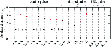 | ||
Fig. 2 Absolute distance error εtest eqn (8d), of the different predicted spectra for test data: double pulses with time delay Td and amplitude ratios A1![[thin space (1/6-em)]](https://www.rsc.org/images/entities/char_2009.gif) : :![[thin space (1/6-em)]](https://www.rsc.org/images/entities/char_2009.gif) A2 as indicated, chirped pules with chirp parameter β, and partially coherent pulses with coherence time τ. A2 as indicated, chirped pules with chirp parameter β, and partially coherent pulses with coherence time τ. | ||
The strongest sensitivity occurs for spectra from chirped pulses where the ones with the most positive chirp (β = +3) are twice as difficult to predict than ones with β = −3. We will come back to this point later. Finally, it is surprising that a spectrum from a partially-coherent pulse, which is naturally very “busy”, can be identified and therefore predicted from the (averaged) fluctuating spectra, even if the coherence time is shorter than that of the noise (τ = 0.5 fs) with similar accuracy as for longer coherence times of the reference spectrum. We will discuss the spectra from the different pulse forms now in detail.
4.1 Prediction of spectra from double pulses
The reference pulse is here given by| fd(t) = Nd[A1GT(t + Td/2) + A2GT(t − Td/2)]cos(ω*t), | (9) |
Fig. 3 shows predicted spectra for exemplary double pulses with pulse shapes indicated in gray. Comparison of black and blue curves also helps to develop a sense for what the quantitative distance errors in Fig. 2 mean for the quality of the predictions. The generally good agreement proves that the training of the network was successful and has generated an accurate map.
 | ||
Fig. 3 Predicted photoelectron spectra (black) are compared to reference spectra (blue, dashed). All spectra are normalized. The corresponding reference pulses (gray) are shown in each panel. In each of the three figure matrices with 3 × 3 panels, time delays Td are 4 fs, 8 fs, and 12 fs, respectively, from left to right; and from top to bottom, pulse amplitude ratios A1![[thin space (1/6-em)]](https://www.rsc.org/images/entities/char_2009.gif) : :![[thin space (1/6-em)]](https://www.rsc.org/images/entities/char_2009.gif) A2 are 1 A2 are 1![[thin space (1/6-em)]](https://www.rsc.org/images/entities/char_2009.gif) : :![[thin space (1/6-em)]](https://www.rsc.org/images/entities/char_2009.gif) 2, 1 2, 1![[thin space (1/6-em)]](https://www.rsc.org/images/entities/char_2009.gif) : :![[thin space (1/6-em)]](https://www.rsc.org/images/entities/char_2009.gif) 1, and 2 1, and 2![[thin space (1/6-em)]](https://www.rsc.org/images/entities/char_2009.gif) : :![[thin space (1/6-em)]](https://www.rsc.org/images/entities/char_2009.gif) 1, respectively, see eqn (9). Left matrix: prediction for a SHM from test data. The SHM is chosen such that Ep ≈ 3.84 × 10¹⁶ W fs cm−2 and each prediction returns an absolute distance (numbers in the panels) Dkref, cf. eqn (8b), within the range of 30–70% in the error distribution. Middle matrix: prediction of noisy 3D helium spectra (composed of the sum of the two relevant angular-momentum channels s and d) through the trained network for pulses of pulse energy Ep = 1.6 × 10¹⁶ W fs cm−2. Right matrix: same as middle matrix but for an energy of Ep = 6.4 × 10¹⁶ W fs cm−2. 1, respectively, see eqn (9). Left matrix: prediction for a SHM from test data. The SHM is chosen such that Ep ≈ 3.84 × 10¹⁶ W fs cm−2 and each prediction returns an absolute distance (numbers in the panels) Dkref, cf. eqn (8b), within the range of 30–70% in the error distribution. Middle matrix: prediction of noisy 3D helium spectra (composed of the sum of the two relevant angular-momentum channels s and d) through the trained network for pulses of pulse energy Ep = 1.6 × 10¹⁶ W fs cm−2. Right matrix: same as middle matrix but for an energy of Ep = 6.4 × 10¹⁶ W fs cm−2. | ||
However, the test data, although not used for training, belong to the same class of SHM that are used for training. A more realistic test is the prediction of a 3D helium spectrum as shown in Fig. 3 (middle), as this is similar to predicting spectra from experimental fluctuating pulses. In general, the prediction works very well, as one can see—only small details of the spectral structures are sometimes not resolved. This is remarkable, as the shapes of the spectra from the same reference pulses are quite different for the 1D system used for training and the 3D helium (compare the individual equivalent panels on the left and in the middle Fig. 3). This confirms the transferability of the network and underlines its interpolation capability.
Predictions become worse for increasing pulse energy as shown in the right part of Fig. 3. This is also true for the test data (not shown) but to a slightly lesser extent. While features are still reproduced, the predicted spectra are in general slightly too wide compared to the reference spectra.
4.2 Prediction of spectra from chirped pulses
The chirped reference pulses are parameterized by β and read| fβ(t) = NβGβ(t)cos(φβ(t)), | (10a) |
 | (10b) |
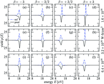 | ||
| Fig. 4 Prediction of 3D helium spectra (black, solid) for chirped pulses, eqn (10). The reference 3D helium spectra are shown with blue dashed lines. | ||
4.3 Prediction of spectra from partially-coherent pulses
We finally will predict spectra from pulses which are themselves “noisy”, i.e., partially coherent and generated according to eqn (1) but for different coherence times τ, typical for SASE FELs. The motivation for such reference spectra was to see where the prediction breaks down since we had the expectation that, at least for spectra from pulses with coherence times much shorter than the ones used for the learning space of fluctuating spectra, the trained network would lose its predictive capability, even more so as the spectra have quite detailed features, see Fig. 5. However, to our surprise this is not the case, as also revealed by the errors given in Fig. 2.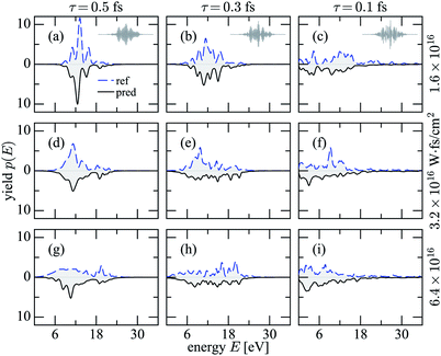 | ||
| Fig. 5 Prediction of 3D helium spectra (black) for partially coherent pulses (1). The reference 3D helium spectra are shown with blue dashed lines. | ||
4.4 Prediction errors for different pulse shapes
Now, we are in the position to understand details of the distance errors εtest in Fig. 2 for reference spectra from different pulse shapes. As one can see from Fig. 6 as a rule of thumb, the smaller the ionization probability Pion (shown in Fig. 6 with blue points), the smaller the diversity of spectra the pulses generate, including reference spectra. All spectra in this section have been analyzed with networks trained with a learning data set of the same size and a common set of input averaged fluctuating spectra. Therefore, one would expect that the average mutual distance![[D with combining macron]](https://www.rsc.org/images/entities/i_char_0044_0304.gif) Ω, defined in eqn (8c), of the reference spectra is larger for a more extended space of highly diverse spectra as compared to a smaller space of less diverse spectra. This is indeed the case as
Ω, defined in eqn (8c), of the reference spectra is larger for a more extended space of highly diverse spectra as compared to a smaller space of less diverse spectra. This is indeed the case as ![[D with combining macron]](https://www.rsc.org/images/entities/i_char_0044_0304.gif) test shown with red points in Fig. 6 reveal: they follow the trend of Pion for the test data. Since it is more difficult for the network to interpolate if the available reference spectra are more distant, one would expect larger errors, which explains the trend of the distance errors in Fig. 2. Particularly striking is the change for chirped pulses:18 negative chirp produces small Pion and in turn a moderate diversity of spectra with relatively small
test shown with red points in Fig. 6 reveal: they follow the trend of Pion for the test data. Since it is more difficult for the network to interpolate if the available reference spectra are more distant, one would expect larger errors, which explains the trend of the distance errors in Fig. 2. Particularly striking is the change for chirped pulses:18 negative chirp produces small Pion and in turn a moderate diversity of spectra with relatively small ![[D with combining macron]](https://www.rsc.org/images/entities/i_char_0044_0304.gif) test, and therefore also the smallest εtest. For positive chirp, the exact opposite holds. One cannot expect that ionization yield, distance of spectra and errors are directly proportional, as the physical process leading from the pulses to the spectra is still non-linear. For instance, long time-delays in double pulses give rise to more diverse spectra than short time-delays. Moreover, the εtest are for predictions from noisy spectra. Yet, the causal chain of Pion →
test, and therefore also the smallest εtest. For positive chirp, the exact opposite holds. One cannot expect that ionization yield, distance of spectra and errors are directly proportional, as the physical process leading from the pulses to the spectra is still non-linear. For instance, long time-delays in double pulses give rise to more diverse spectra than short time-delays. Moreover, the εtest are for predictions from noisy spectra. Yet, the causal chain of Pion → ![[D with combining macron]](https://www.rsc.org/images/entities/i_char_0044_0304.gif) test → εtest holds.
test → εtest holds.
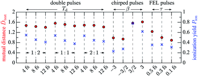 | ||
Fig. 6 Properties of test reference spectra for the pulses from Fig. 2. Average ionization yield Pion (blue, right axis) and average mutual distance ![[D with combining macron]](https://www.rsc.org/images/entities/i_char_0044_0304.gif) test (red, left axis). test (red, left axis). | ||
This section has shown that the trained networks can predict spectra from widely varying pulse forms well. The effort one has to invest into the deep neural networks for the prediction of the spectra depends on the diversity of spectra a certain pulse form is capable of generating.
5 Single-shot noisy double pulses: simultaneous purification of spectra and reconstruction of time-delay
The analysis of the previous section has prepared us for the final goal of this work, namely purifying the spectra while simultaneously extracting the correct time-delay from spectra recorded with noisy double pulses which have an unknown time-delay within a certain interval. This scenario is motivated by SASE XFEL pulses,19 where the pulse is either split by a chicane for the relativistic electron bunch, which creates the light pulse, or by situations where an XFEL pulse and a time-delayed strong laser pulse are used together, whereby the delay between the two pulses is characterized by a jitter from shot to shot.We model fluctuating double pulses with noise-free double pulses and admixture of noisy double pulses,
| fdq(t) = Ndq[GT(t + Td/2) + GT(t − Td/2)][cos(ω*t) + qFτ(t)], | (11) |
Since so far we have not extracted the time-delay of the pulses from the spectra, we verify in Section 5.1, that it is possible to identify the time-delay of double pulses from noise-free spectra generated by those pulses. In Section 5.2 we will address fluctuating spectra. We first determine the pulses’ time-delay Td encoded in single-shot spectra generated with noisy double pulses. Subsequently, we average the single-shot spectra with identified Td over small intervals of time-delay (1 fs) and purify these averaged spectra. Recall, that purifying means that we remove the fluctuations from spectra by predicting the spectra generated from the respective noise-free pulse forms, in the present case from the noise-free double pulses.
5.1 Extraction of time-delay from spectra generated with double pulses
Here, we aim at constructing a network-based map to extract the time-delays Td of double pulses from the (noise-free) spectra the pulses fd0 from eqn (11) generate. To this end we have generated a learning data set of spectra from 20![[thin space (1/6-em)]](https://www.rsc.org/images/entities/char_2009.gif) 000 SHMs, each paired with a single double pulse fd0(t) with delays between 2 and 14 fs. The learning data is distributed into training, validation and test data as before (see Section 3.3), and the network is also that of Section 3.3, but the number of neurons on each layer is 50, the learning rate is 0.008 and the number of epochs is 200.
000 SHMs, each paired with a single double pulse fd0(t) with delays between 2 and 14 fs. The learning data is distributed into training, validation and test data as before (see Section 3.3), and the network is also that of Section 3.3, but the number of neurons on each layer is 50, the learning rate is 0.008 and the number of epochs is 200.
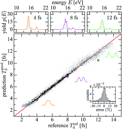
Fig. 7 shows the training success with the SHMs as well as the transfer of the network to unknown 3D helium spectra. The trained network reproduces well the delays (results scatter along the ideal red line with an error given in the inset). For short Td the results deviate from the ideal line since the individual pulses in the double pulse have a width of T = 3 fs which limits the resolution towards small time-delays. Results for the reconstructed time-delay for full 3D helium spectra are given for Td of 4, 8, and 12 fs, respectively, and demonstrate the transferability of the network. The upper row shows the corresponding 3D helium spectra. Given the similarity of these spectra for different time-delays it is remarkable that the trained network can reliably extract the time-delays. We may conclude that we can map out the delay of the pulse from the spectrum it has produced with the help of the trained network.
5.2 Purification of single-shot spectra and simultaneous extraction of the time-delay of the generating double pulse
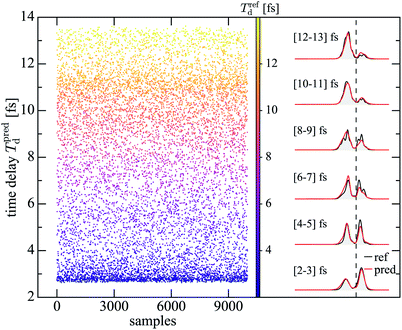
Finally, we analyze noisy single-shot spectra with the goal to purify them as in Section 4 and to extract the time delay of the generating double pulse as in Section 5.1, simultaneously. In order to have reasonable statistics for the map and also reasonably different spectra for different time delays, we reconstruct from each noisy single-shot spectrum (all for the same SHM) the time-delay but average the spectra afterwards over small intervals (1 fs) of time-delays. Subsequently, the averaged spectra are passed through another trained network to purify them. The result is shown in Fig. 8. The scattered points are reconstructed time-delays coloured with the reference time-delays. The even change in color demonstrates that the reconstruction of time-delays for the test data has been successful. The spectra within 1 fs intervals of reconstructed time-delays are averaged and subsequently purified. They are shown on the right in red along with reference spectra (black), averaged over the same interval of time-delays. The generally good agreement demonstrates that reconstruction of time-delays and purification of the single-shot spectra is possible without additional information over the single-shot spectra.The last step is to prove that the reconstruction and purification can be transferred to spectra unknown to the networks. To this end we take noisy single-shot spectra of 3D helium with three well-defined time-delays and pass them through the trained network for reconstruction of the time-delay. The scattered points in Fig. 9 show the reconstructed time-delays. We average the corresponding spectra over 1 fs around the three peak time-delays in the scattered points and pass the averaged spectra through the purification network to arrive at the three spectra on the right in red. They agree well with the corresponding reference spectra, averaged over the same intervals of time-delay (black). Hence, the trained networks should be able to reconstruct the time-delay and purify the corresponding fluctuating experimental spectra as they are produced by SASE FELs.
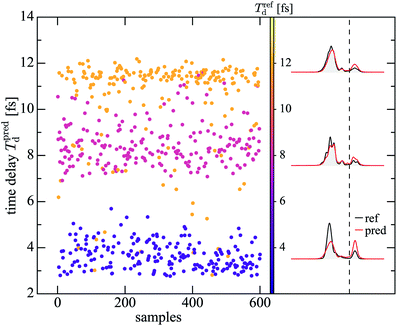 | ||
| Fig. 9 Same as Fig. 8 but for 3D helium for which the network was not trained. The distribution of predicted time-delays shows three main peaks at 4, 8, and 12 fs. The single-shot spectra are averaged over all spectra with time-delays in an interval of 1 fs about the three peaks. The averaged spectra are passed through the trained network to obtain the corresponding purified spectra shown on the right (red). The three averaged reference spectra (black) are obtained in the same way. | ||
6 Conclusions
To summarize, we have devised a strategy to create maps through deep neural networks between fluctuating nonlinear photo-ionization spectra and noise-free spectra, and between fluctuating single-shot spectra and pulse properties. A crucial part of this strategy is the formulation of synthetic Hamilton matrices which describe artificial systems, similar to ones existing in reality. We use the SHM to generate a sufficient amount of spectra for training the network. In a first application6 we purified fluctuating spectra as typically produced by SASE FELs through a neural-network-based map.Here, we have taken this mapping capability to a new level by predicting from fluctuating spectra—which should come ultimately from experiment—the spectra which would be obtained with specific noise-free pulses, namely double pulses, chirped pulses and chaotic (partially-coherent) pulses. While generally the prediction works as well as the purification (prediction) for simple Gaussian pulses, the error analysis has revealed interesting differences for the different pulse shapes.
In a second application we have constructed a neural-network-based map which can extract the time-delay of double pulses from fluctuating single-shot spectra generated by those noisy double pulses. Finally, we could demonstrate that suitably trained networks can achieve both, purification and extraction of the time-delay, from fluctuating single-shot spectra as typically produced by SASE FELs. Clearly, neural networks open promising new ways to analyze particular noisy data with a potential which has been by far not exhausted.
Conflicts of interest
There are no conflicts to declare.Acknowledgements
We acknowledge financial support by “BiGmax”, the Max Planck Society’s research network on big-data-driven materials science, and by “QUTIF”, a priority program (no. 1840) of the Deutsche Forschungsgemeinschaft. Open Access funding was provided by the Max Planck Society.Notes and references
- V. Dunjko and H. J. Briegel, Rep. Prog. Phys., 2018, 81, 074001 CrossRef
.
- P. Mehta, M. Bukov, C.-H. Wang, A. G. R. Day, C. Richardson, C. K. Fisher and D. J. Schwab, Phys. Rep., 2019, 810, 1 CrossRef
.
- G. Carleo, I. Cirac, K. Cranmer, L. Daudet, M. Schuld, N. Tishby, L. Vogt-Maranto and L. Zdeborová, 2019, arXiv:1903.10563.
- R. Selle, T. Brixner, T. Bayer, M. Wollenhaupt and T. Baumert, J. Phys. B: At., Mol. Opt. Phys., 2008, 41, 074019 CrossRef
.
- A. Sanchez-Gonzalez, P. Micaelli, C. Olivier, T. R. Barillot, M. Ilchen, A. A. Lutman, A. Marinelli, T. Maxwell, A. Achner, M. Agåker, N. Berrah, C. Bostedt, J. D. Bozek, J. Buck, P. H. Bucksbaum, S. C. Montero, B. Cooper, J. P. Cryan, M. Dong, R. Feifel, L. J. Frasinski, H. Fukuzawa, A. Galler, G. Hartmann, N. Hartmann, W. Helml, A. S. Johnson, A. Knie, A. O. Lindahl, J. Liu, K. Motomura, M. Mucke, C. O’Grady, J.-E. Rubensson, E. R. Simpson, R. J. Squibb, C. Såthe, K. Ueda, M. Vacher, D. J. Walke, V. Zhaunerchyk, R. N. Coffee and J. P. Marangos, Nat. Commun., 2017, 8, ncomms15461 CrossRef
.
- S. K. Giri, U. Saalmann and J. M. Rost, Phys. Rev. Lett., 2020, 124, 113201 CrossRef
.
- J. White and Z. Chang, Opt. Express, 2019, 27, 4799 CrossRef CAS
.
- Z. Zhu, J. White, Z. Chang and S. Pang, Sci. Rep., 2020, 10, 1 CrossRef CAS
.
- R. Ziv, A. Dikopoltsev, T. Zahavy, I. Rubinstein, P. Sidorenko, O. Cohen and M. Segev, Opt. Express, 2020, 28, 7528 CrossRef
.
- X. Liu, G. Zhang, J. Li, G. Shi, M. Zhou, B. Huang, Y. Tang, X. Song and W. Yang, Phys. Rev. Lett., 2020, 124, 113202 CrossRef CAS
.
- T. Pfeifer, Y. Jiang, S. Düsterer, R. Moshammer and J. Ullrich, Opt. Lett., 2010, 35, 3441 CrossRef
.
- R. Moshammer, T. Pfeifer, A. Rudenko, Y. H. Jiang, L. Foucar, M. Kurka, K. U. Kühnel, C. D. Schröter, J. Ullrich, O. Herrwerth, M. F. Kling, X.-J. Liu, K. Motomura, H. Fukuzawa, A. Yamada, K. Ueda, K. L. Ishikawa, K. Nagaya, H. Iwayama, A. Sugishima, Y. Mizoguchi, S. Yase, M. Yao, N. Saito, A. Belkacem, M. Nagasono, A. Higashiya, M. Yabashi, T. Ishikawa, H. Ohashi, H. Kimura and T. Togashi, Opt. Express, 2011, 19, 21698 CrossRef CAS
.
-
F. Chollet, Keras: The Python deep learning library, https://keras.io, 2015 Search PubMed
.
- B. Hanin, Mathematics, 2019, 7, 992 CrossRef
.
- D. P. Kingma and J. L. Ba, 2017, arXiv:1412.6980 [cs].
- S.-i. Amari, N. Fujita and S. Shinomoto, Neural Comput., 1992, 4, 605 CrossRef
.
- J. Hestness, S. Narang, N. Ardalani, G. Diamos, H. Jun, H. Kianinejad, M. M. A. Patwary, Y. Yang and Y. Zhou, 2017, arXiv:1712.00409 [cs, stat].
- U. Saalmann, S. K. Giri and J. M. Rost, Phys. Rev. Lett., 2018, 121, 153203 CrossRef CAS
.
- A. Marinelli, D. Ratner, A. A. Lutman, J. Turner, J. Welch, F.-J. Decker, H. Loos, C. Behrens, S. Gilevich, A. A. Miahnahri, S. Vetter, T. J. Maxwell, Y. Ding, R. Coffee, S. Wakatsuki and Z. Huang, Nat. Commun., 2015, 6, 6369 CrossRef CAS
.
| This journal is © The Royal Society of Chemistry 2021 |

