Unsupervised structure classes vs. supervised property classes of silicon quantum dots using neural networks

Abstract

Machine learning classification is a useful technique to predict structure/property relationships in samples of nanomaterials where distributions of sizes and mixtures of shapes are persistent. The separation of classes, however, can either be supervised based on domain knowledge (human intelligence), or based entirely on unsupervised machine learning (artificial intelligence). This raises the questions as to which approach is more reliable, and how they compare? In this study we combine an ensemble data set of electronic structure simulations of the size, shape and peak wavelength for the optical emission of hydrogen passivated silicon quantum dots with artificial neural networks to explore the utility of different types of classes. By comparing the domain-driven and data-driven approaches we find there is a disconnect between what we see (optical emission) and assume (that a particular color band represents a special class), and what the data supports. Contrary to expectation, controlling a limited set of structural characteristics is not specific enough to classify a quantum dot based on color, even though it is experimentally intuitive.

---

New concepts

One of the challenges in using artificial intelligence to explore the relationships between the processing, structure, properties and performance of nanoscale materials is deciding how much domain knowledge to include, and how much to trust the data. Too much domain knowledge introduces bias that makes machine learning outcomes unreliable; too little domain knowledge and machine learning outcomes are esoteric and difficult to act upon. Using interpretable machine learning methods makes combining domain knowledge and data-driven outcomes more compatible but knowing how and when to insert scientific insights into the process is still problematic. Using “black-box” neural networks is even more problematic, since these uninterpretable methods give no insight into how out domain knowledge is being used (or ignored). Applying domain knowledge at the outset, setting the scene for machine learning to confirm to refute a prior scientific assumption based on the data is one approach that can be used both with interpretable and uninterpretable methods. Here we directly compare both supervised and unsupervised approaches and use artificial neural networks to see if a the data supports the scientific assumption that the size and shape can definitely determine which colour of the electromagnetic spectrum will be emitted by silicon quantum dots.

Fluorescent silicon quantum dots (SiQDs) are an extremely attractive material for a broad range of optoelectronic applications. SiQDs-based LEDs were first reported¹ in the near-infra-red, followed by the visible red range^2,3 and then yellow-green.⁴ White-light silicon-based LED devices which combine red emission from silicon nanocrystals with blue-green emission from a luminescent polymer region have also been reported.⁵ Enhanced control over the optical properties of SiQDs and their distributions should allow new technological applications for silicon as an optoelectronic material. SiQDs may be readily fabricated by a wide variety of means in solid, liquid, gas and plasma-phase methods,^6,7 exhibiting a variety of size and shape distributions^13–15 depending on formation method and conditions.^16,17

For many applications, an increased level of control over nanoparticle shape and the exposure of different surface facets is strongly desirable.^6,8,9 For applications in photovoltaics,¹⁰ for example, nanostructured silicon has attractive properties including relatively low cost, low toxicity, and the possibility of multiple exciton generation.¹¹ Silicon quantum dots may be produced via different methods with various shapes including cubes,¹³ octahedra,¹⁴ truncated octahedra¹⁵ and most commonly pseudo-spheres (deltoidal icositetrahedra), depending on production method and thermodynamic conditions. Shape-engineered nanoparticles may allow more control of optical properties (particularly those involving surface plasmon resonances), while selective functionalization of different surfaces may allow catalytic and self-assembling properties of nanoparticles to be exploited.¹² However, in most cases samples are not perfectly monodispered and distributions in size and variations on the principle shapes are persistent, and strategies that are tolerant of some imprecision are highly desirable.

The optimal morphologies for freestanding hydrogen-terminated SiQDs have been explored using electronic structure simulations,^16,17 reporting that shapes including subsets of the (111), (100) and (113) facets may be formed depending on thermodynamic conditions, consistent with observations of shapes obtained via gas-phase pyrolysis of silane,^14,15 while plasma-based methods¹³ tend to form cubic shapes which maximise the amount of surface hydrogen absorption. The color of the optical emission from each of these types of shapes, at a range of sizes, has also been computed.¹⁸ In a statistical study it with was further reported that, regardless of the distribution in size, certain shapes consistently provide an increase in the spectral resolution, while others consistently show a reduction in spectral resolution, with respect to a diverse mixture lacking shape control. For example, a slightly “rounded” cube, with the corners truncated in the 〈111〉 direction, and the edges truncated in the 〈110〉 direction shows an increase in spectral quality between 42% and 118%, with almost no change in the emission wavelength unless the SiQDs have a Boltzmann distribution at low energy.¹⁹

Since it has been established that there is a relationship between the size, shape and optical emission, it is possible to generate a reliable structure/property relationship using machine learning.^20–24 However, these relationships typically require high level of structural control and have a low tolerance for imprecision. Recent studies have shown that the separation of nanoparticles into classes that naturally contain some distributions and mixtures prior to regression can predict class/property relationships that are just as powerful, but more forgiving.^25,26 There are, however, two approaches to the separation of classes: one based on domain knowledge (human intelligence) informed by the property in question,²⁵ and the other based entirely on machine learning (artificial intelligence) informed by the structural characteristics alone.²⁶ The former is a supervised approach, and the latter unsupervised, and it is unclear at this stage which is the most useful in practice. Should we look for the structural characteristics of classes based on the interpretation of properties, or measure the properties of classes based on their structural characteristics? This is a significant question if the goal is a SiQD with a particular color, but we only have control on the size and the shape.

In this study we combine an ensemble data set of electronic structure simulations of the size-, shape and peak wavelength for the characteristic optical emission of hydrogen passivated SiQDs with artificial neural networks to explore the utility of classes. We compare two classification schemes, based on the properties or the structures, and find that the optical structure/property relationship is remarkably intolerant to the structural flexibility afforded by classes, regardless of the approach.

The data set used in this study contains 303 hydrogen-terminated SiQDs with a diameter between 0.5 nm and 3 nm, and a large range of different morphologies defined by zonohedrons enclosed by {100}, {110}, {111} and {113} facets. These are the four lowest energy H-terminated surface facets, and enclose the range of lowest energy morphologies.¹⁶ SiQDs in the data are labeled by their shapes based on the fraction of each surface facet which they present. Pure {100}, {110}, {111} and {113}-faceted SiQDs are labeled cubes (C), octahedra (OH), rhombic dodecahedra (RD) and deltoidal icositetrahedra (DI) respectively. SiQDs presenting two facets are named with the base name of the majority facet and described as being truncated by the other. SiQDs with three different facets are labeled doubly-truncated versions of the shape described by the majority facet. No SiQD in the data set presents more than three surface facets. All SiQD geometries in the data set were terminated with hydrogen so that each silicon atom was tetrahedrally fourfold coordinated prior to relaxation. This data set is freely available for download.²⁷ Although this is a small data set, it is exhaustive with respect to the structural features, and the results will show that we can obtain high quality and reliable classification results using the chosen methods.

The features used in this study were the average diameter (D), the average Si–Si coordination number (n_coord), the fraction of {111} facet area (f(111)), {110} facet area (f(110)), {100} facet area (f(100)) and {113} facet area (f(113)). These facets have been shown to be important experimentally.¹⁵ We also created a new feature, the hydrogen to silicon ratio (HSi_ratio) that captures information about the size, shape and surface chemistry simultaneously. All of these features have been chosen because they are accessible, and assessable, using standard experimental instruments, such as an electron microscope. We first scaled the data with a robust scaler and normalized the data between 0 and 1, then checked for strongly correlated variables. The concentration of silicon and (surface) hydrogen were found to have over 90% correlation to the diameter (see ESI†) and so were dropped in favor of the diameter which is more experimentally assessable. This is to be expected, since the hydrogen resides on the surface and the surface-to-volume ratio is a well known feature of nanoparticles, routinely calculated in phenomenological models and measured experimentally using thermogravimetric analysis (TGA) to determine the amount of coating on the surface of the nanoparticle. Similarly the n_coord was found to the strongly correlated to HSi_ratio and so was dropped in favour of HSi_ratio which retains information about the surface chemistry in the feature space.

We then separated the SiQDs into clusters, using either an unsupervised clustering method based entirely on the structural features (the artificial intelligence approach), or a supervised separation based on the property label (the human intelligence approach). In the later case we recognised that the human eye sees color over wavelengths ranging roughly from 400 nanometers (violet) to 700 nanometers (red), and the accepted bands of visible light are: violet from 400–450 nm (666–789 THz frequency), blue from 450–495 nm (605–666 THz frequency), green from 495–570 nm (526–605 THz frequency), yellow from 570–590 nm (508–526 THz frequency), orange from 590–620 nm (486–508 THz frequency), and red from 620–750 nm (400–486 THz frequency). SiQDs with an emission wavelength shorter than 400 nm where removed as outliers. This provides 6 color bands and the SiQDs where grouped accordingly, referred to as supervised property classes, as shown in Fig. 1. The distribution of each of these bands with respect to each of the structural features are shown in the ESI.†

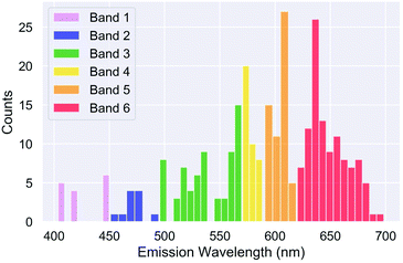Fig. 1 Distribution of the supervised property classes (color bands) with respect to the optical emission wavelength, λ (nm).

In the former case we undertook supervised clustering using a new clustering method referred to as Iterative Label Spreading²⁸ (ILS) that has the advantage of including hyper-parameter optimization which in absent in other unsupervised clustering algorithms.²⁹ ILS is based on a general definition of a cluster and the quality of a clustering result, and is capable of predicting the number and type of clusters and outliers in advance of clustering, regardless of the complexity of the distribution of the data or the size and shape of clusters. ILS calculates the ordered minimum distance (R_min(i)) between data instances in the high dimensional space, as described in detail in ref. 28, such that the R_min(i) plot gives a one dimensional representation of density in the feature space from which the number of clusters can be automatically extracted (by identifying discontinuities between clusters that divide the plot into n regions). Discontinuities separating clusters can be identified by hand or automatically using a continuous wavelet transform peak finding algorithm with smoothing over p points, which essentially sets the minimum cluster size to identify clusters of no smaller than p. In this case we considered p = 15, so that each cluster was required to contain at least 5% of the data. One point can be relabelled in each region (preferably in a dense region i.e. several grouped minima) to run ILS again, and obtain a fully labeled data set with n clusters defined. ILS can also be applied to each individual cluster to confirm that each region is a single cluster that should not be divided further. It has been shown to be more reliable than alternative approaches for simple and challenging cases (such as the null and chain cases) and to be ideal for studying noisy data with high dimensionality and high variance, as is typical for nanoparticle systems.^26,30 This software is freely available online.³¹

The results of the ILS clustering are shown in Fig. 2, where we can see the ordered minimum distance plot in Fig. 2(a) with the re-labeled minima used to re-rerun ILS and assign each SiQD to a cluster. Fig. 2(b) shows the minimum distance plot colored by the assigned cluster, recognized by the density discontinuities. This provides 6 clusters based on the structural features alone, referred to as unsupervised structure classes. The distribution of each of these clusters with respect to each of the structural features are shown in the ESI.† These cluster assignments, while not informatic in their own right, can be used as target labels for during classification.

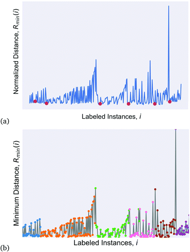Fig. 2 (a) Initialised minimum distance (R_min(i)) plot using iterative label spreading (ILS), and (b) the R_min(i) plot showing discontinuities between the clusters which are coloured for clarity.

The next step is to determine if these bands and clusters constitute formal SiQD classes, which are separable based on the structural characteristics alone. There are a variety of classification methods that can be applied to the prediction of nanomaterial structure/property relationships; each with advantages and disadvantages.³² In each of these cases we have used a multi-layer perceptron and optimised the hyper-parameters using a random search over 5000 trials, including the number of hidden layers and the number of neurons per layer. The supervised property classes where separated using a three layer neural network with: {activation = ‘identity’, solver = ‘lbfgs’, max_iter = 230, alpha = 0.4339, learning_rate = ‘constant’, hidden_layer_sizes = (10,7,3), early_stopping = True, random_state = 42}. Using these hyper-parameters the training score for the supervised classes was R_train² = 0.975, the testing score was R_test² = 0.933 and the cross validation score based on 10-fold cross validation was R_CV² = 0.96 ± 0.084. The unsupervised structure classes where separated using a two layer neural network with: {activation = ‘relu’, solver = ‘lbfgs’, max_iter = 297, alpha = 0.0451, learning_rate = ‘invscaling’, hidden_layer_sizes = (4,3), early_stopping = True, random_state = 42}. Using these hyper-parameters the training score for the supervised classes was R_train² = 1.000, the testing score was R_test² = 0.983 and the cross validation score based on 10-fold cross validation was R_CV² = 0.98 ± 0.10.

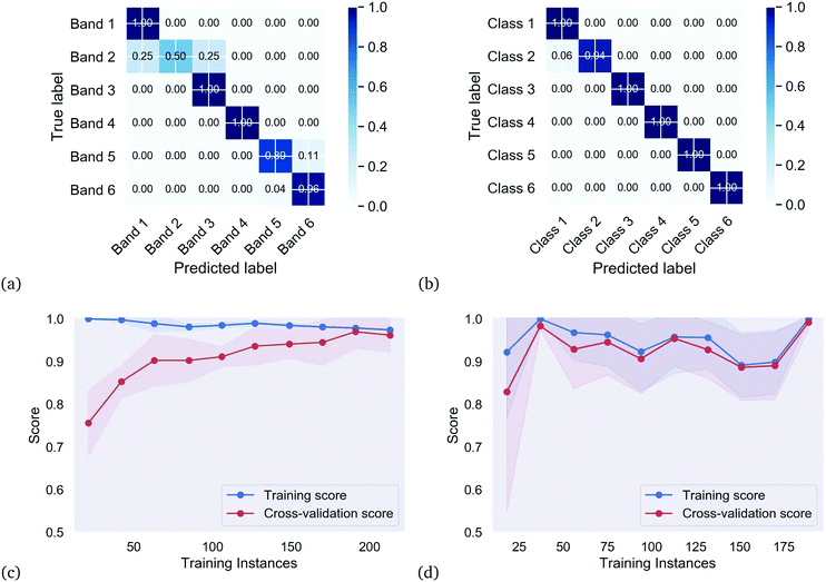
The results of the classification are summarized by the classification reports in Table 1, and captured in Fig. 3. Precision is the ratio of correctly predicted positive observations to the total predicted positive observations, recall is the ratio of correctly predicted positive observations to the all observations in actual class, and accuracy (measured here using the F1-score) is simply a ratio of correctly predicted observation to the total observations. The F1-score = 2 × ((precision × recall)/(precision + recall)). Fig. 3 includes the two confusion matrices showing the normalized fractions of true positives, true negatives, false positives and false negatives for each combination of supervised property classes determined using domain knowledge (Fig. 3(a)), and the unsupervised structure classes determined using iterative label spreading (ILS) clustering (Fig. 3(b)), along with their learning curves showing the overall accuracy and generalizability for the supervised (Fig. 3(c)) and unsupervised (Fig. 3(d)) approaches.

Table 1 Classification reports for the supervised property classes determined using domain knowledge, and the unsupervised structure classes determined using iterative label spreading (ILS) clustering

Supervised property classes					Unsupervised structure classes
Class	Precision	Recall	F1-score	SiQDs	Class	Precision	Recall	F1-score	SiQDs
Band 1	0.75	1.00	0.86	15	Cluster 1	0.80	1.00	0.89	48
Band 2	1.00	0.50	0.67	11	Cluster 2	1.00	0.94	0.97	83
Band 3	0.92	1.00	0.96	67	Cluster 3	1.00	1.00	1.00	62
Band 4	1.00	1.00	1.00	38	Cluster 4	1.00	1.00	1.00	43
Band 5	0.89	0.89	0.89	58	Cluster 5	1.00	1.00	1.00	36
Band 6	0.96	0.96	0.96	108	Cluster 6	1.00	1.00	1.00	25

---

Fig. 3 Confusion matrices for the supervised property classes determined using domain knowledge (a), and the unsupervised structure classes determined using iterative label spreading (ILS) clustering (b), along with their learning curves showing the overall accuracy and generalisability for the supervised (c) and unsupervised (d) cases.

As expected, the unsupervised classes, determined based on the structural features, can be well separated based on these features alone. This neural network has excellent precision and recall, meaning that if the size, shape of surface passivated SiQDs are known (either from simulations or electron microscopy) then they can be definitively placed into a class. The weights and biases for this classifier are provided in the ESI.† Unfortunately, as shown in Fig. 4 these classes have no bearing on optical emission. None of the structural classes exhibit spectral purity.

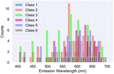Fig. 4 Distribution of the unsupervised structure classes (clusters) with respect to the optical emission wavelength, λ (nm).

In the case of the supervised property classes we can see from left side of Table 1 that, although they are very flexible and able to represent highly non-linear relationships, the neural network struggles to distinguish the supervised Band 1 (violet) and Band 2 (blue), and Band 5 (orange) and Band 6 (red), based on the features. Bands 1 and 2 have very low numbers of SiQDs and working under the assumption that there were insufficient instances to separate these classes a neural network the bands were then separated using a random forest classifier (see ESI†), but the results were worse and the random forest classifier can only distinguish Band 6 (red). It could be that a larger set of SiQDs could overcome this issue, but this data set is complete in the sense that it represents all possible silicon structures which can be formed by symmetric cutting with any combination these planes around the centrosymmetric lattice site.¹⁶ There simply are no other structures with this set of surfaces in this size range. A larger set would mean extending the size beyond the largest 3.04 nm structure (but below the exciton Bohr radius of 5 nm to ensure quantum confinement³³) which is challenging for some electronic structure methods and too computationally demanding for some researchers. The learning curve has also converged with respect to the size of the training set, suggesting more data will not help.

The alternative interpretation is that it is just not possible to rely on structural characteristics to classify what we know from domain knowledge; that there is a structure/property relationship determining the optical emission of SiQDs. This observation is not class-dependent, and attempts to purify SiQDs based on their color will always result in in a mixture of sizes and shapes, but not as a separable class (even though we see them that way). Conversely, although it is possible to definitively classify SiQDs into different types of structures, which may be viable targets for synthesis, the classes are not optically pure. Strategies to tune the optical emission by controlling the structure must be very precise to be useful, as there is no tolerance for the imperfection afforded by classes as we had hoped.

To test this final hypothesis we have used the artificial neural network to perform regression on the SiQD data set, to predict the emission wavelength label as a function of the retained structural features. This optimized network used: {activation = ‘relu’, solver = ‘lbfgs’, max_iter = 270, alpha = 4.652, learning_rate = ‘invscaling’, hidden_layer_sizes = (10,3), early_stopping = True, random_state = 42}. With these hyper-parameters the training score was R_train² = 0.997, the testing score was R_test² = 0.996 and the cross validation score based on 10-fold cross validation was R_CV² = 0.994 ± 0.007. The results are shown in Fig. 5, along with the learning curve, and the weights and biases are provided in the ESI.†

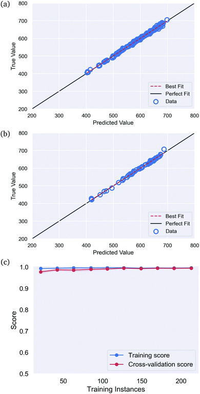Fig. 5 The results predicting the optical emission spectrum for SiQDs, in the (a) training set, (b) testing set, and (c) the cross validation set, showing no over-fitting or under-fitting.

Here we can see that, although the supervised property classes cannot be distinguished by the neural network classifier based on the structural features (a class/property relationship), the more specific structure/property relationship can be accurately modelled by the neural network regressor. There is a strong structure/property relationship, but not an intuitive class-dependent one.

We can conclude from this study that machine learning is capable of classifying silicon quantum dots based on their structure, and predicting the very strong connection between the structure and the optical properties to guide experimental design. There is however a disconnect between what we see (optical emission) and assume (that a particular color band represents a special class), and what the data supports. Although we see distinct colors, and know that there is a relationship to the size and shape, the quantum dots that return a particular color are not a class unto themselves. Shape controlled synthesis must be holistic, controlling both the size and all the surface orientations simultaneously to provide the precision needed make a color that we want. Focussing on one structural characteristic of another may be sufficient to make quantum dots that look the same and occupy a certain class, but classes are not specific enough to emit in a certain color.

Conflicts of interest

There are no conflicts of interest to declare.

Acknowledgements

Computational resources for this project have been supplied by the National Computing Infrastructure (NCI) national facility under MAS Grant p00.

References

1. K. Y. Cheng, R. Anthony, U. R. Kortshagen and R. J. Holmes, Nano Lett., 2010, 10, 1154–1157.
2. D. P. Puzzo, E. J. Henderson, M. G. Helander, Z. Wang, G. A. Ozin and Z. Lu, Nano Lett., 2011, 11, 1585–1590.
3. K. Y. Cheng, R. Anthony, U. R. Kortshagen and R. J. Holmes, Nano Lett., 2011, 11, 1952–1956.
4. F. Maier-Flaig, J. Rinck, M. Stephan, T. Bocksrocker, M. Bruns, C. Kübel, A. K. Powell, G. A. Ozin and U. Lemmer, Nano Lett., 2013, 13, 475–480.
5. B. Ghosh, Y. Masuda, Y. Wakayama, Y. Imanaka, J. Inoue, K. Hashi, K. Deguchi, H. Yamada, Y. Sakka, S. Ohki, T. Shimizu and N. Shirahata, Adv. Funct. Mater., 2014, 24, 7151–7160.
6. L. Mangolini, J. Vac. Sci. Technol., B, 2013, 31, 020801.
7. S. Askari, M. Macias-Montero, T. Velusamy, P. Maguire, V. Svrcek and D. Mariotti, J. Phys. D: Appl. Phys., 2015, 48, 314002.
8. S. Chinnathambi, S. Chen, S. Ganesan and N. Hanagata, Adv. Healthcare Mater., 2014, 3, 10–29.
9. X. Cheng, S. B. Lowe, P. J. Reece and J. J. Gooding, Chem. Soc. Rev., 2014, 43, 2680–2700.
10. S. Dutta, S. Chatterjee, K. Mallem, Y. H. Cho and J. Yi, Renewable Energy, 2019, 144, 2–14.
11. M. C. Beard, K. Knutsen, P. R. Yu, J. Luther, Q. ong, W. Metzger, R. J. Ellingson and A. J. Nozik, Nano Lett., 2007, 7, 2506.
12. M. Abdelhameed, D. R. Martir, S. Chen, W. Z. Xu, O. O. Oyeneye, S. Chakrabarti, E. Zysman-Colman and P. A. Charpentier, Sci. Rep., 2018, 8, 3050.
13. L. Mangolini, U. Kortshagen and A. Bapat, J. Nanopart. Res., 2006, 2007, 39–52.
14. T. U. M. S. Murthy, N. Miyamoto, M. Shimbo and J. Nishizawa, J. Cryst. Growth, 1976, 33, 1–7.
15. R. Körmer, B. Butz, E. Spiecker and W. Peukert, Cryst. Growth Des., 2012, 12, 1330–1336.
16. H. F. Wilson and A. S. Barnard, J. Phys. Chem. C, 2014, 118, 2580–2586.
17. H. F. Wilson and A. S. Barnard, Cryst. Growth Des., 2014, 14, 4468–4474.
18. H. F. Wilson, L. McKenzie-Sell and A. S. Barnard, J. Mater. Chem. C, 2014, 2, 9451–9456.
19. A. S. Barnard and H. F. Wilson, J. Phys. Chem. C, 2015, 119, 7969–7977.
20. K. Rajan, Annu. Rev. Mater. Res., 2008, 38, 299–322.
21. J. Jain, S. P. Ong, G. Hautier, W. Chen, W. D. Richards, S. Dacek, S. Cholia, D. Gunter, D. Skinner, G. Ceder and K. A. Persson, APL Mater., 2013, 1, 011002.
22. T. Lookman, F. J. Alexander and K. Rajan, Information science for materials discovery and design, Springer Series in Materials Science, Springer International Publishing, Switzerland, 2016.
23. L. Ward and C. Wolverton, Curr. Opin. Solid State Mater. Sci., 2017, 21, 167–176.
24. D. M. Dimiduk, E. A. Holm and S. R. Niezgoda, Int. Matter. Manufact. Innov., 2018, 7, 157–172.
25. C. A. Feigl, B. Motevalli, A. J. Parker, B. Sun and A. S. Barnard, Nano. Horiz., 2020, 4, 983–990.
26. A. J. Parker, G. Opletal and A. S. Barnard, J. Appl. Phys., 2020, 128, 014301.
27. A. Barnard and H. Wilson, Silicon Quantum Dot Data Set, v2, CSIRO Data Collection, 2015 DOI:10.4225/08/5721BB609EDB0.
28. A. J. Parker and A. S. Barnard, Adv. Theory Simul., 2019, 2, 1900145.
29. D. Xu and Y. Tian, Ann. Data Sci., 2015, 2, 165.
30. A. J. Parker and A. S. Barnard, Nano. Horiz., 2020, 5, 1394–1399.
31. A. Barnard and A. Parker, Iterative Label Spreading, v1, CSIRO Software Collection, 2019 DOI:10.25919/5d806280b91a9.
32. A. S. Barnard, B. Motevalli, A. J. Parker, J. M. Fisher, C. A. Feigl and G. Opletal, Nanoscale, 2019, 11, 19190–19201.
33. E. G. Barbagiovanni, D. J. Lockwood, P. J. Simpson and L. V. Goncharova, Appl. Phys. Rev., 2014, 1, 011302.

---

Footnote

† Electronic supplementary information (ESI) available: The correlation matrix and skew map; the distribution of the supervised property classes (color bands) and the distribution of the unsupervised property classes (ILS clusters); the weights and biases for the neural networks, and the entire workflow diagram. See DOI: 10.1039/d0nh00637h

---