 Open Access Article
Creative Commons Attribution 3.0 Unported Licence
Beyond structural insight: a deep neural network for the prediction of Pt L2/3-edge X-ray absorption spectra†
Luke
Watson
 ,
Conor D.
Rankine
 and
Thomas J.
Penfold
 *
*
Chemistry – School of Natural and Environmental Sciences, Newcastle University, Newcastle, upon Tyne, NE1 7RU, UK. E-mail: tom.penfold@ncl.ac.uk
First published on 31st March 2022
Abstract
X-ray absorption spectroscopy at the L2/3 edge can be used to obtain detailed information about the local electronic and geometric structure of transition metal complexes. By virtue of the dipole selection rules, the transition metal L2/3 edge usually exhibits two distinct spectral regions: (i) the “white line”, which is dominated by bound electronic transitions from metal-centred 2p orbitals into unoccupied orbitals with d character; the intensity and shape of this band consequently reflects the d density of states (d-DOS), which is strongly modulated by mixing with ligand orbitals involved in chemical bonding, and (ii) the post-edge, where oscillations encode the local geometric structure around the X-ray absorption site. In this Article, we extend our recently-developed XANESNET deep neural network (DNN) beyond the K-edge to predict X-ray absorption spectra at the Pt L2/3 edge. We demonstrate that XANESNET is able to predict Pt L2/3 -edge X-ray absorption spectra, including both the parts containing electronic and geometric structural information. The performance of our DNN in practical situations is demonstrated by application to two Pt complexes, and by simulating the transient spectrum of a photoexcited dimeric Pt complex. Our discussion includes an analysis of the feature importance in our DNN which demonstrates the role of key features and assists with interpreting the performance of the network.
1 Introduction
Interest in machine learning (used as an umbrella term for a variety of statistical algorithms that build predictive or decision-capable models based on inferences from data) has surged in recent years as a consequence of fundamental advances in deep learning algorithms [especially deep neural networks (DNNs)],1 the increased accessibility of high-performance computational hardware, and the proliferation of large data sets.2–4 In chemistry,5 machine-learning models have the potential to be able to make fast, accurate, and affordable predictions of properties and observables, sometimes with very little external input, and they are consequently very appealing for a broad range of applications including materials,6–10 catalyst,11–14 and drug design,15,16 chemical reaction prediction,17–21 and atomistic modelling.22–27Spectroscopy is central to research across the natural sciences and in engineering, being one of the most effective methods for characterising the properties of molecules and materials. This has led to the development of a number of approaches aimed at exploiting machine learning for data reduction, prediction, and/or analysis, in addition to accelerating theoretical calculations of electronically-excited states and spectra.28–42 In particular, and the focus of this Article, the X-ray regime provides valuable element- and site-specific information on the geometric, electronic, and spin structure of matter and, consequently, a number of recent works have addressed directly the development of models for the prediction and analysis of X-ray absorption spectra.43–65
These approaches can be subdivided into two categories: (i) “forward” (i.e. property/structure-to-spectrum) and (ii) “reverse” (i.e. spectrum-to-property/structure) mappings. The latter is perhaps the more natural of the two, in some sense, as it has a clear connection to the problem that X-ray spectroscopists face day-to-day in their work: how can a measurement/observable be interpreted? However, direct extraction of three-dimensional structure in the “reverse” mapping approach cannot be achieved without constraints due to the limited resolution of X-ray spectra and, consequently, most approaches have focused on deriving key structural parameters, e.g. oxidation state, coordination number, or morphology, among others. In addition, for the analysis of complicated, disordered, and dynamical systems, it is very unlikely that deriving a single three-dimensional structure from an X-ray spectrum would be physically meaningful. In such a situation, high-throughput (i.e. fast, accurate, and affordable) theory is needed to enable large-scale configurational sampling using the “forward” mapping approach.
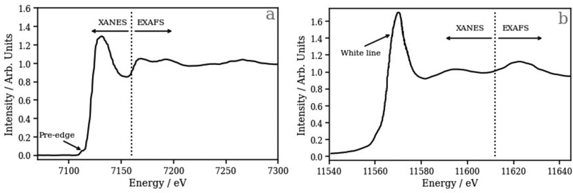
To address this, we have recently developed43,47 and applied45,46 a deep neural network (DNN) based on the simple multilayer perceptron (MLP) model that has been able to model accurately and affordably the K-edge X-ray absorption spectra of transition metal complexes. Our DNN predicts peak positions with sub-eV accuracy and peak intensities with errors over an order of magnitude smaller than the spectral variations that the model is engineered to capture from no input beyond geometric information about the local environment of the X-ray absorption site.43,47 With the ability to predict ca. 1000 XANES spectra per second using off-the-shelf commercial-grade hardware (an AMD Ryzen Threadripper 3970X CPU; 3.7–4.5 GHz), our DNN provides a significant reduction in computational expense compared to first-principles/ab initio simulations that facilitates large-scale configurational sampling. In the context of the present work, it is important to note that transition metal K-edge XANES spectra are dominated by post-edge oscillations relating directly to structural features via the scattering of X-ray photoelectrons (Fig. 1a). In contrast, by virtue of the dipole selection rules, transition metal L2/3 edge XANES spectra, especially those corresponding to 5 d elements such as Pt, as studied here, usually exhibit two distinct spectral regions: (i) the “white line”, which is dominated by bound electronic transitions from metal-centred 2p orbitals into unoccupied orbitals with d character; the intensity and shape of this band consequently reflects the d density of states (d-DOS), which is strongly modulated by mixing with ligand orbitals involved in chemical bonding, and (ii) the post-edge, where oscillations encode the local geometric structure around the X-ray absorption site (Fig. 1b).
In this Article, we extend our recently-developed DNN43,47 beyond the K-edge to predict XANES spectra at the Pt L2/3 edge with a view towards exploring whether it is possible for the present framework to predict accurately the electronic, as well as the structural, features of the L2/3 edge. Importantly, although there has been significant development in the first-principles/ab initio treatment of L2/3 edge XANES spectra,66–73 it remains a challenging task to develop (statistical) model-based approaches. While (machine-learning) models for K-edge X-ray spectroscopy are advancing at pace, fewer model-based approaches have been developed to target the L2/3 edge. Recent work by Lueder is one such example, which has seen the introduction of models structured around a multiplet-theory-based approach and demonstrated that they are effective for predicting L2/3-edge X-ray absorption spectra for first-row transition metal complexes.74,75 Through the use of multiplet theory, Lueder's approach focused on the electronic, rather than structural, components of the L2/3 edge XANES spectra.74,75 We demonstrate that our DNN, trained on theoretical spectra, and using local geometric information around the absorption site, is able to predict Pt L2/3 edge XANES spectra including both the parts dominated by electronic and geometric structural information. The performance of our DNN in a practical situation is demonstrated by application to two Pt complexes and by prediction of the transient spectrum of a dimeric Pt complex. Our discussion includes an analysis of the feature importance in our DNN which demonstrates the role of key features and assists with interpreting the performance of the network.
2 Theory and computational details
2.1 Dataset and multiple scattering theory calculations
Our reference dataset comprises Pt X-ray absorption site geometries (“samples”) derived from 6530 Pt-containing structures harvested from the transition metal Quantum Machine (tmQM)76,77 dataset with the corresponding L2/3 edge XANES spectra (“labels”) calculated in-house using multiple scattering theory (MST) as implemented in the FDMNES package.78,79 530 samples from the reference dataset were isolated at random to form a “held-out” testing dataset (evaluated post-optimisation only). The remaining samples comprised the training and validation datasets used during optimisation. The average L2/3 edge XANES spectra and the variance over this subset of samples is shown in Fig. S1 (ESI†). The training and validation subsets were constructed “on-the-fly” throughout via repeated K-fold cross validation with five repeats and five folds, i.e. a five-times-repeated 80![[thin space (1/6-em)]](https://www.rsc.org/images/entities/char_2009.gif) :
:![[thin space (1/6-em)]](https://www.rsc.org/images/entities/char_2009.gif) 20 split.
20 split.
The Pt L2/3-edge XANES MST calculations employed a self-consistent muffin-tin-type potential of radius 6.0 Å around the X-ray absorbing site, and the interaction with the X-ray field was described using the electric quadrupole approximation. Relativistic effects, including spin–orbit coupling (SOC; implemented following the approach of Wood and Boring in ref. 80) were integrated into the Pt L2/3 edge XANES MST calculations to split the L2 and L3 edges.
In this Article, three different sets of target XANES spectra were used, each differing in the preprocessing applied to the calculated absorption cross-sections. The first case, where the absorption cross-sections were used as obtained from FDMNES without any preprocessing, we refer to as the unconvoluted/non-broadened model. The second case, where the calculated absorption cross-sections were convoluted/broadened with a simple, fixed-width Lorentzian function [full-width-at-half-maximum (FWHM) = 0.5 eV], we refer to as the Lorentzian-broadened model. The final case, which represents the typical preprocessing strategy for theoretical spectra, we refer to as the arctan-broadened model; here, the calculated absorption cross-sections were convoluted with an energy-dependent arctangent function to account for various factors including the core-hole-lifetime broadening, instrument response, and many-body effects, e.g. inelastic losses. This particular kind of convolution was carried out following an empirical model close to the Seah-Dench formalism81 as detailed in ref. 43. All reference datasets associated with this work are publicly available; refer to the Data Availability Statement for details.
2.2 Deep neural network
The general architecture of the current-generation XANESNET DNN is described in detail in ref. 47 we recommend this reference to the unfamiliar reader. The code is publicly available under the GNU Public License (GPLv3) on GitLab.82Briefly, the architecture is based on the deep multilayer perceptron (MLP) model and comprises an input layer, two hidden layers, and an output layer. All layers are dense, i.e. fully connected, and each hidden layer performs a nonlinear transformation using the rectified linear unit (relu) activation function. The input layer comprises 129 neurons (to accept a feature vector of 129 symmetry functions encoding the local environment around an X-ray absorption site), the hidden layers each comprise 512 neurons, and the output layer comprises 1100 neurons from which the discretised L2/3 edge XANES spectrum is retrieved, i.e. XANESNET is a multi-output MLP with each output neuron corresponding to the spectral intensity at a given energy gridpoint. The inputs – local environments around X-ray absorption sites – are encoded via dimensionality reduction using the weighted atom-centered symmetry function (wACSF) descriptor of Gastegger and Marquetand et al.83
The internal weights, W, are optimised via iterative feed-forward and backpropagation cycles to minimise the empirical loss, J(W), defined here as the mean-squared error (MSE) between the predicted, μpredict, and target, μtarget, L2/3 -edge XANES spectra. Gradients of the empirical loss with respect to the internal weights, δJ(W)/δW, were estimated over minibatches of 32 samples and updated iteratively according to the Adaptive Moment Estimation (ADAM) algorithm. The learning rate for the ADAM algorithm was set to 1 × 10⁻⁴.
Regularization was implemented to minimize the propensity of overfitting; batch standardization and dropout were applied at each hidden layer. The probability, p, of dropout was set to 0.25.
The XANESNET DNN is programmed in Python 3 with the TensorFlow84/Keras85 API and integrated into a Scikit-Learn86 (sklearn) data pre- and post-processing pipeline via the KerasRegressor wrapper for Scikit-Learn. The Atomic Simulation Environment87 (ase) API is used to handle and manipulate molecular structures.
3 Results and discussion
3.1 Deep neural network evaluation
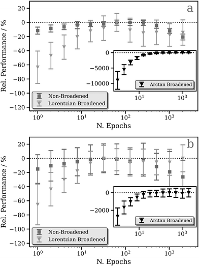
Fig. 2a and b show the relative performance of our DNN (i.e. the percentage difference in the performance of the model relative to the best-performing model for that figure panel) at the Pt L2 and L3 edges, respectively, as a function of number of training cycles (“epochs”). We have evaluated three models which differ in the way that the L2/3 edge XANES spectra are preprocessed, i.e. in the choice of target function (see Theory and computational details).The first (the “unconvoluted/non-broadened” model) is optimised with the calculated absorption cross-section as the target function. As shown in Fig. S2 (ESI†), these target functions exhibit sharp resonances characteristic of bound–bound (e.g. d ← 2p) transitions, especially in the region close to the X-ray absorption edge, arising from the high density of 5d ← 2p transitions. At the Pt L2 and L3 edges, this model shows very limited, near-negligible improvement (<10%) as a function of the number of epochs (Fig. 2). This is a consequence of the challenges that our DNN faces in learning the multitude of sharp resonances in the pre-edge and around the “white line”. Indeed, in the simple MLP model, each individual neuron in the output layer of a multi-output network is independent; here, each represents a discretised energy point in the Pt L2/3 edge XANES spectrum (see Theory and computational details). However, the narrow nature of these resonances means that small spectral shifts can transfer the entire intensity from one output neuron to another. From the perspective of our DNN, this represents a very large change in the target output, but it is in fact one that could be induced with a very small change in the input – the local geometric structure around the absorption site. This can lead to a breakdown in the correlation between inputs (i.e. structures) and outputs (i.e. spectra) reducing the effectiveness of learning. In addition, the objective of the DNN during training is to minimise the loss/cost function (here, the MSE; see Theory and computational details); given the challenges of modelling the sharp resonances in the pre-edge and around the “white line”, the DNN focuses on this region throughout training as it has the largest effect on the MSE. This can lead to poorer performance for predictions of the above-ionisation resonances in the post-edge. On this basis, we conclude that this first model is inappropriate for the Pt L2/3 edge (cf. the situation at the K edge; see ref. 43), and so we discard it at this point – we will not consider it again in this Article.
To address this situation, a second model was optimised with fixed-width-Lorentzian-broadened (FWHM = 0.5 eV) absorption cross-sections as the target functions. This second model shows a stronger improvement as a function of the number of epochs; a ca. 60% improvement is observed at the Pt L2 (Fig. 2a) and L3 (Fig. 2b) edges. A third model was also optimised (inset in Fig. 2) in which the calculated absorption cross-sections were preprocessed via broadening with the energy-dependent arctangent function described in ref. 43. Illustrative example spectra can be seen in Fig. S2 (ESI†). This third model shows a much greater relative change in performance as a function of the number of epochs, likely a consequence of the lower resolution of the target function post-convolution. The average MSE converges towards ca. 1.0 × 10⁻⁴ and, given that the MSE from the first few epochs (ca. 1.0 × 10⁻²) is orders of magnitude greater, this model consequently exhibits a huge percentage-wise improvement in performance at the Pt L2 (Fig. 2a) and L3 (Fig. 2b) edges.
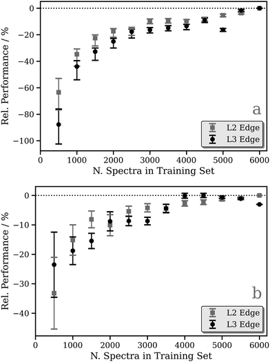
Focusing on the fixed-width-Lorentzian- and arctan-broadened models, Fig. 3 shows the relative performance of our DNN as a function of the number of samples in the training dataset. For both the fixed-width-Lorentzian- (Fig. 3a) and arctan-broadened (Fig. 3b) models, a percentage-wise improvement of ca. 50% is observed over an increase in the size of the training set from ca. 500 to 6000 samples. A comparable improvement is observed for both the Pt L2 and L3 edges. Fig. S3–S6 (ESI†) show six DNN-predicted and theoretical Pt L2/3 edge XANES spectra presented for the purpose of comparison; in each Figure, the upper and lower three panels contain selections from the top and bottom 1% of DNN predictions, respectively, where predictions are ranked by MSE. In both the Lorentzian- and arctan-broadened models, the top 1% of DNN predictions are essentially indistinguishable from the target Pt L2 and L3 edge XANES spectra.
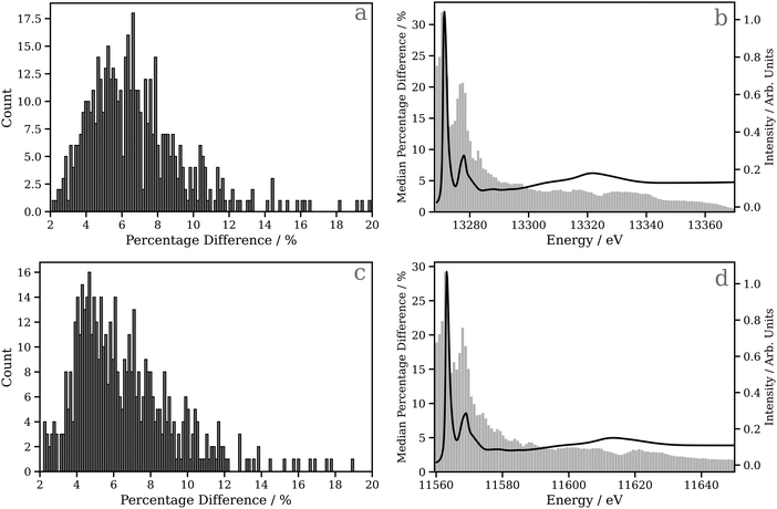
Fig. 4a and c show percentage error between the target and the actual spectrum achieved on DNN predictions of Pt L2 and L3 edge XANES spectra, respectively, for the 530 held-out samples in the testing dataset. Here, the absorption cross-sections have been broadened with a fixed-width Lorentzian function (FWHM = 0.5 eV); the corresponding data for the absorption cross-sections broadened with the energy-dependent arctangent function are shown in Fig. S7 (ESI†). For the Pt L2 edge (Fig. 4a), the median percentage error is 4.827, and the lower and upper quartiles are found at 6.386 and 8.080, respectively, while for the Pt L3 edge (Fig. 4c), the median percentage error is 4.605, and the lower and upper quartiles are found at 6.013 and 7.973, respectively. In Fig. 4b and d, bar charts of the median percentage error point-by-point are overlaid on averaged Pt L2 and L3 edge XANES spectra, respectively. These figures show that the error is largest in the region of the spectrum near the edge/“white line”. This is likely the consequence of two primary factors: (i) the edge/“white line” region of the spectrum is the most structured and, therefore, the most challenging for the DNN, and (ii) the input, i.e. the local (geometric) environment around the X-ray absorption site, is purely structural and does not encode electronic information (e.g. orbital structure) directly. One would expect this additional information to be valuable for predictions in this region of the XANES spectrum given the electronic nature of the resonances (cf. the above-ionisation resonances in the post-edge).
3.2 Predicting the Pt L2/3 edge XANES of zerovalent Pt complexes
A key application of L2/3 edge XANES is to probe directly, by virtue of the dipole selection rules, the unoccupied d valence orbitals, which can provide insight into the electronic structure and chemical bonding framework of the complex under study. One example from organometallic chemistry is to interpret chemical bonding within the framework of the Dewar–Chatt–Duncanson model,88,89i.e. in the context of σ donation and π back-donation between the transition metal and the ligands. Indeed, transition metal L2/3 edge XANES has been used to describe the bonding in organometallic complexes within this framework in a number of previous studies.90–92Here, we test the performance of our DNN by predicting the Pt L3 edge XANES spectra of two zerovalent Pt molecules:93,94 [Pt(PH3)2 (η2-C2H4)] and [Pt(PH3)2 (η2-C2 (CN)4)] (shown in Fig. 5a and b, respectively). As previously demonstrated by Dias, Fonseca, and Herbst,95 the “white lines” of these spectra are an effective measure of the π* strength of the C2H4 and C2 (CN)4 ligands coordinated to the Pt(PPh3)2 fragment. Fig. 6 shows Pt L3 edge DNN predictions (solid lines) for [Pt(PH3)2 (η2-C2H4)] and [Pt(PH3)2 (η2-C2(CN)4)] compared to the experimental Pt L3 edge XANES spectra (dashed lines). For both [Pt(PH3)2 (η2-C2H4)] and [Pt(PH3)2 (η2-C2(CN)4)], strong qualitative agreement of the spectral shape is observed with both the edge and post-edge resonances captured, albeit with the latter being slightly too intense in the Pt L3 -edge DNN predictions relative to the experimental traces. In terms of the electronic properties of the complexes, the Pt 5d-DOS can be interpreted using the edge jump (E0; located at the inflection point of the rising edge) and the edge maximum (Emax) of the “white line”. If we assume, as in the aforementioned work,95 that E0 reflects the energy of the highest-occupied molecular orbital (HOMO) and Emax reflects the energy of the lowest-unoccupied molecular orbital (LUMO), the HOMO–LUMO gap can be estimated as Emax − E0.96,97 In addition - because the aforementioned work95 has established that the HOMO is dominated by Pt dπ-orbitals and the LUMO by π* orbitals for these complexes – this energy difference can be related to the dπ-orbital interaction energy, ΔEπ, and manifests as a doublet growth in the second derivative of the spectra shown for the DNN predictions in Fig. S8 (ESI†). ΔEπ, as determined from our DNN predictions, is found to be ca. 4 and 6 eV for [Pt(PH3)2 (η2-C2H4)] and [Pt(PH3)2 (η2-C2(CN)4)], respectively; values that are in excellent agreement with their experimentally-determined counterparts: ca. 4 and 7 eV for [Pt(PH3)2 (η2-C2H4)] and [Pt(PH3)2 (η2-C2(CN)4)], respectively.95
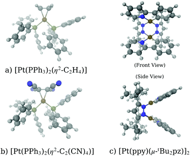 | ||
| Fig. 5 Schematics of the molecules studied in the work: (a) [Pt(PH3)2 (η2-C2H4)], (b) [Pt(PH3)2 (η2-C2(CN)4)], and (c)[Pt(ppy)(μ-tBu2 pz)]2. | ||
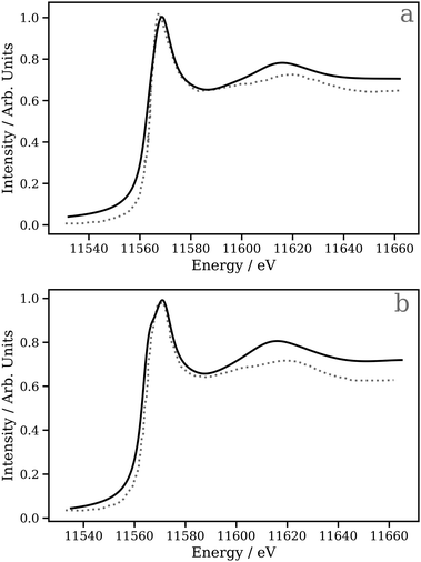 | ||
| Fig. 6 The Pt L3 edge XANES spectra of (a) [Pt(PH3)2 (η2 -C2H4)] and (b) [Pt(PH3)2 (η2 -C2(CN)4)]. The dashed lines are experimental Pt L3 edge XANES spectra digitised from ref. 95 and the solid lines are DNN predictions. | ||
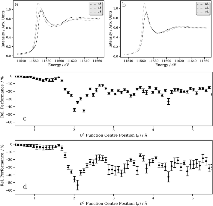
A deeper understanding can be provided by a “shell-by-shell”98,99 simulation (a simulation in which the number of neighboring atoms around the X-ray absorption site is gradually increased by incorporating an increasing number of radial “shells” up to the point of convergence) which also provides, in parallel, an opportunity to assess the performance of our DNN compared to first-principles/ab initio simulations carried out using the FDMNES package (i.e. does our model capture the expected physics?). Fig. 7a and b show the “shell-by-shell” simulation for [Pt(PH3)2 (η2-C2(CN)4)] using FDMNES and our DNN, respectively. Increasing the radius from 2 Å to 4 Å and, ultimately, 6 Å leads to a reduction of the “white line” intensity and an increase in intensity of the post-edge resonance at ca. 11![[thin space (1/6-em)]](https://www.rsc.org/images/entities/char_2009.gif) 610 eV. The change in the “white line” intensity reflects the mixing of the Pt d-DOS with ligand orbitals, which serves to broaden and, consequently, reduce the spectral intensity. The change in the post-edge resonance occurs from scattering from the surrounding ligands. The changes observed in the first-principles/ab initio FDMNES simulations are captured consistently and qualitatively well by our DNN, which is encouraging.
610 eV. The change in the “white line” intensity reflects the mixing of the Pt d-DOS with ligand orbitals, which serves to broaden and, consequently, reduce the spectral intensity. The change in the post-edge resonance occurs from scattering from the surrounding ligands. The changes observed in the first-principles/ab initio FDMNES simulations are captured consistently and qualitatively well by our DNN, which is encouraging.
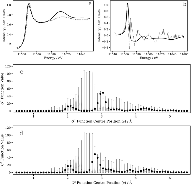
The ability of our DNN to capture the correct behaviour in the “shell-by-shell” simulation depends, to an extent, on the sensitivity of each radial (G2-type) input feature in the wACSF feature vector (see Theory and computational details). Fig. 7c and d show plots of the inference feature importance for the individual G2-type symmetry functions at the Pt L2 and L3 edges, respectively, obtained by assessing the performance penalty (Rel. Performance) when randomising the input featurewise, i.e. each point represents one of the 64 G2 type symmetry functions in the wACSF feature vector, and the relative performance hit when randomising that feature reflects the evaluated importance of the feature to the DNN at inference time. A similar trend is observed at the Pt L2 and L3 edges, with the strongest sensitivity observed at ca. 2–3 Å. This corresponds approximately to the first and second coordination spheres for the Pt-containing organometallic complexes in the tmQM76,77 dataset. It consequently explains the strong change observed when expanding the shell from 2 to 4 Å in the DNN “shell-by-shell” simulation and the weaker effect when expanding the shell from 4 to 6 Å (Fig. 7b).
3.3 Predicting the effect of excited-state distortions in a Pt dimer
In this second case study, we focus on the excited-state structure of a dinuclear Pt(II) complex with tert-butyl substituted pyrazolate bridging units: [Pt(ppy)(μ-tBu2pz)]2 (Fig. 5c; ppy = 2-phenylpyridine; tBu2pz = 3,5-di-tert-butylpyrazolate) – a complex previously studied by Lockard et al.100 Indeed, there has been extensive work carried out using time-resolved X-ray techniques on diplatinum transition metal complexes with a view towards elucidating the electronic and geometric structural changes upon photoexcitation.66,101–104Fig. 8a shows the Pt L3 edge XANES spectrum of [Pt(ppy)(μ-tBu2pz)]2 in the electronic ground state. The DNN prediction reproduces the shape of the experimental Pt L3 edge XANES spectrum with good qualitative agreement in terms of position and intensity, particularly in the “white-line” region yet, although the energetic position of the post-edge resonance is in good agreement with experiment, it is slightly too intense. One potential reason for this is that [Pt(ppy)(μ-tBu2pz)]2], having two Pt atoms, is irregular given the content of the training dataset (otherwise exclusively mono-Pt complexes); predictions for [Pt(ppy)(μ-tBu2pz)]2 could be considered to be beyond the scope of the present model. To investigate this possibility, Fig. 8c is presented; a violin plot of the distribution of G2-type symmetry function values included within the training set is shown in this figure, and the scatter markers show the G2-type symmetry function values associated with the wACSF vector describing [Pt(ppy)(μ-tBu2pz)]2 at the electronic ground-state geometry. Fig. 8c shows that the G2 symmetry functions describing the environment at an ca. 3 Å radial distance (corresponding to the Pt–Pt distance) are at the edge of, or outside, the range of values found in the training dataset, which could suggest that the model may be less reliable here. For reference, Fig. S9 (ESI†) shows a histogram of atom types and their respective distances from the Pt X-ray absorption sites in the training dataset used in this work.
Fig. S10 (ESI†) shows the influence of the second Pt atom on the DNN predictions and first-principles/ab initio FDMNES simulations. For the latter, there is limited effect. While this may be surprising, it is nonetheless consistent with previous analysis on a diplatinum system66 which showed that the spectral feature at 11.610 keV is not strongly affected by the second Pt atom but, instead, results from scattering from the first and second coordination shells around each Pt X-ray absorption site.66 In contrast, the DNN predictions show a large reduction in intensity in this feature when removing the second Pt atom, illustrating the effect of its presence is overestimated in our present model – again, likely because it differs considerably from the content of our current training dataset.
Next, we investigate the transient Pt L3 edge XANES spectrum, i.e. the difference XANES spectrum between the excited-state and ground-state Pt L3 edge XANES spectra.105,106 This represents a larger challenge for our DNN as both spectra have to be described accurately in order to reproduce the experimentally-acquired transient. Fig. 8b shows both the experimentally-acquired and DNN-predicted transient Pt L3 edge XANES spectra. The experimental XANES spectrum (digitised from ref. 100) was acquired 100 ps post-photoexcitation of [Pt(ppy)(μ-tBu2pz)]2 with 527 nm light at a time after which the complex is expected to have relaxed into its lowest-energy triplet (T1) excited state.100 The first positive feature in the experimentally-acquired transient (located at ca. 11565 eV) arises from a 5d ← 2p electronic transition driven by the photoexcitation, while the remaining features observed in the experimentally-acquired transient reflect structural changes.100 As observed in Fig. 8b, our DNN-predicted transient is in poor agreement with the experimentally-acquired transient and, above the positive transition at ca. 11560 eV, shows only very weak changes. It is possible to rationalise this from Fig. 8d, which not only shows that the G2-type symmetry function values encoding information on the Pt–Pt distance for the T1-state complex are at the edge of range of values contained in the training dataset (and, in any case, dinuclear Pt complexes are not contained in the training dataset), but – crucially – that the change in Pt–Pt distance post-photoexcitation moves the interaction into a region where our DNN is less sensitive to changes in geometry [i.e. the feature importance is comparatively low around ca. 2.5–2.7 Å (T1 state) as opposed to ca. 2.9–3.1 Å (S0 state); Fig. 7c and d]. Compounding the difficulties faced here, the structural changes of the complex otherwise are small (≤0.03 Å). We therefore expect that the inadequate simulation of the experimentally-acquired transient is largely due to these factors, and this dinuclear Pt(II) complex clearly falls outside the scope of the presently-developed model.
4 Conclusions
In this Article, we have developed and applied a DNN to predict accurately and affordably Pt L2/3-edge XANES spectra. In contrast to our previous work43–47 at the transition metal K edges, the L2/3-edge XANES spectra exhibit a larger and more direct sensitivity to the electronic structure of the absorbing atom owing to the dipole-allowed bound–bound 5d ← 2p electronic transitions. In contrast, at the transition metal K-edges, electronic transitions into the unoccupied d-DOS are dipole forbidden and form only a weak pre-edge region in the K-edge XANES spectra. This has brought into focus a key question: does our input representation, based entirely on the geometric structure, remain reliable and encode the necessary information for a ‘forward’ mapping of the structure onto the L2/3-edge XANES spectral features?We have demonstrated that, using a small training dataset of 6000 local absorption sites and Pt L2/3-edge XANES spectra, it is possible to develop a DNN with a simple architecture, very similar to our previous transition metal K-edge DNNs,43,47 which is effective for predicting Pt L2/3 edge XANES spectra, as demonstrated on 530 held-out testing dataset samples. However, a key difference from our previous work43–47 at the transition metal K edges is that, here, our DNN is ostensibly unable to learn from absorption cross-sections without preprocessing since the L2/3 edge exhibits very structured, sharp resonance peaks characteristic of bound-bound transitions. This challenge is addressable by applying either a fixed-width Lorentzian or arctangent convolutional broadening to each calculated L2/3 edge XANES spectrum prior to training. While both show effective learning, the latter option is the less desirable of the two as it presumes a specific (instrument) resolution, while this can (and generally does) vary between different experimental techniques [e.g. when using high-energy-resolution fluorescence detection (HERFD)107 spectroscopy]. Consequently, to maintain the generality of our DNN at the L2/3 edge, we have focused on the former preprocessing strategy for training the model and, as for the transition metal K edges, made available the option to apply a tailored artangent convolutional broadening as an post-processing step.
In terms of the performance of our DNN at the Pt L2/3 edge, we have shown that the largest percentage differences are observed in the “white line”/edge region of the XANES spectrum: the part which is dominated by electronic transitions and is probably poorly predicted without explicit electronic information being supplied to our DNN. This potentially highlights a limitation of our current encoding strategy: it is based entirely on geometric information about the local environment around the absorption site. At the transition metal K edge, the majority of the features in the XANES spectrum are above-ionisation resonances which arise through interferences of the scattered X-ray photoelectrons and, here, the direct link to between structure and spectrum (necessary for a physical ‘forward’ mapping) is clear. In contrast, at the L2/3 edge, there is a substantially larger contribution from electronic characteristics and, while there is still an implicit link between the geometric properties of the local environment around the absorption site and the electronic structure of the complex, it is not as direct.
We applied our DNN to two test examples: (i) predicting the Pt L2/3 -edge XANES of zerovalent Pt complexes, and (ii) predicting the Pt L2/3-edge transient corresponding to excited-state distortions in a Pt dimer. For the latter, we demonstrated that when poor agreement between our DNN predictions and the experimentally-acquired transient arose, this could be traced back to the details of the model and, in particular, the contents of the training dataset. Indeed, any artificial learning model will only ever be as good as the data used to train it. Consequently, future work in this area needs to focus on bespoke training datasets for (transition metal) X-ray absorption spectroscopy, tailored to maximise the sensitivity of the model(s) to the particular problem(s).108
Data availability
The data supporting this publication are openly available under an Open Data Commons Open Database License. Additional metadata are available at 10.25405/data.ncl.17206706.Conflicts of interest
There are no conflicts to declare.Acknowledgements
The research described in this paper was funded by the Leverhulme Trust (Project RPG-2020-268) and EPSRC (EP/S022058/1, EP/R021503/1, and EP/R51309X/1). CDR is supported by a Doctoral Prize Fellowship (EP/R51309X/1). This research made use of the Rocket High Performance Computing (HPC) service at Newcastle University. CDR additionally thanks the Alan Turing Institute, via which access to the EPSRC-supported (EP/T022205/1) Joint Academic Data Science Endeavour (JADE) HPC cluster was provided under Project JAD029.Notes and references
- Y. Lecun, Y. Bengio and G. Hinton, Nature, 2015, 521, 436–444 CrossRef CAS PubMed
.
- M. I. Jordan and T. M. Mitchell, Science, 2015, 349, 255–260 CrossRef CAS PubMed
.
-
S. Shalev-Shwartz and S. Ben-David, Understanding Machine Learning: From Theory to Algorithms, Cambridge University Press, 2014 Search PubMed
.
-
M. Mohri, A. Rostamizadeh and A. Talwalkar, Foundations of Machine Learning, MIT Press, 2018 Search PubMed
.
- A. C. Mater and M. L. Coote, J. Chem. Inf. Model., 2019, 59, 2545–2559 CrossRef CAS PubMed
.
- K. T. Schütt, H. Glawe, F. Brockherde, A. Sanna, K.-R. Müller and E. K. Gross, Phys. Rev. B: Condens. Matter Mater. Phys., 2014, 89, 205118 CrossRef
.
- B. Meredig, A. Agrawal, S. Kirklin, J. E. Saal, J. W. Doak, A. Thompson, K. Zhang, A. Choudhary and C. Wolverton, Phys. Rev. B: Condens. Matter Mater. Phys., 2014, 89, 094104 CrossRef
.
- K. T. Butler, D. W. Davies, H. Cartwright, O. Isayev and A. Walsh, Nature, 2018, 559, 547–555 CrossRef CAS PubMed
.
- W. Sun, Y. Zheng, K. Yang, Q. Zhang, A. A. Shah, Z. Wu, Y. Sun, L. Feng, D. Chen and Z. Xiao,
et al.
, Sci. Adv., 2019, 5, eaay4275 CrossRef CAS PubMed
.
- S. Chibani and F.-X. Coudert, APL Mater., 2020, 8, 080701 CrossRef CAS
.
- Z. Li, X. Ma and H. Xin, Catal. Today, 2017, 280, 232–238 CrossRef CAS
.
- Z. Li, S. Wang, W. S. Chin, L. E. Achenie and H. Xin, J. Mater. Chem. A, 2017, 5, 24131–24138 RSC
.
- J. R. Kitchin, Nat. Catal., 2018, 1, 230–232 CrossRef
.
- A. F. Zahrt, J. J. Henle, B. T. Rose, Y. Wang, W. T. Darrow and S. E. Denmark, Science, 2019, 363, eaau5631 CrossRef CAS PubMed
.
- R. Burbidge, M. Trotter, B. Buxton and S. Holden, Compr. Chemom., 2001, 26, 5–14 CrossRef CAS
.
- V. D. Mouchlis, A. Afantitis, A. Serra, M. Fratello, A. G. Papadiamantis, V. Aidinis, I. Lynch, D. Greco and G. Melagraki, Int. J. Mol. Sci., 2021, 22, 1676 CrossRef PubMed
.
- M. H. Segler and M. P. Waller, Chem. – Eur. J., 2017, 23, 5966–5971 CrossRef CAS PubMed
.
- J. S. Schreck, C. W. Coley and K. J. Bishop, ACS Cent. Sci., 2019, 5, 970–981 CrossRef CAS PubMed
.
- V. H. Nair, P. Schwaller and T. Laino, CHIMIA Int. J. Chem., 2019, 73, 997–1000 CrossRef CAS PubMed
.
- D. P. Kovács, W. McCorkindale and A. A. Lee, Nat. Commun., 2021, 12, 1–9 CrossRef PubMed
.
- P. Schwaller, A. C. Vaucher, T. Laino and J.-L. Reymond, Mach. Learn.: Sci. Technol., 2021, 2, 015016 CrossRef
.
- Z. Li, J. R. Kermode and A. De Vita, Phys. Rev. Lett., 2015, 114, 096405 CrossRef PubMed
.
- S. Chmiela, A. Tkatchenko, H. E. Sauceda, I. Poltavsky, K. T. Schütt and K.-R. Müller, Sci. Adv., 2017, 3, e1603015 CrossRef PubMed
.
- K. T. Schütt, M. Gastegger, A. Tkatchenko, K. R. Müller and R. J. Maurer, Nat. Commun., 2019, 10, 1–10 CrossRef PubMed
.
- K. T. Schütt, P. Kessel, M. Gastegger, K. A. Nicoli, A. Tkatchenko and K. R. Müller, J. Chem. Theory Comput., 2019, 15, 448–455 CrossRef PubMed
.
- F. Noé, A. Tkatchenko, K.-R. Müller and C. Clementi, Annu. Rev. Phys. Chem., 2020, 71, 361–390 CrossRef PubMed
.
- M. Bogojeski, L. Vogt-Maranto, M. E. Tuckerman, K.-R. Müller and K. Burke, Nat. Commun., 2020, 11, 1–11 CrossRef PubMed
.
- W. Fu and W. S. Hopkins, J. Phys. Chem. A, 2018, 122, 167–171 CrossRef CAS PubMed
.
- K. Ghosh, A. Stuke, M. Todorović, P. B. Jørgensen, M. N. Schmidt, A. Vehtari and P. Rinke, Adv. Sci., 2019, 6, 1801367 CrossRef PubMed
.
- W. Hu, S. Ye, Y. Zhang, T. Li, G. Zhang, Y. Luo, S. Mukamel and J. Jiang, J. Phys. Chem. Lett., 2019, 10, 6026–6031 CrossRef CAS PubMed
.
- Y. Zhang, Q. Tang, Y. Zhang, J. Wang, U. Stimming and A. A. Lee, Nat. Commun., 2020, 11, 1–6 CrossRef PubMed
.
- B. X. Xue, M. Barbatti and P. O. Dral, J. Phys. Chem. A, 2020, 124, 7199–7210 CrossRef CAS PubMed
.
- J. Westermayr, M. Gastegger, M. F. Menger, S. Mai, L. González and P. Marquetand, Chem. Sci., 2019, 10, 8100–8107 RSC
.
- J. Westermayr and P. Marquetand, Mach. Learn.: Sci. Technol., 2020, 1, 043001 CrossRef
.
- J. Westermayr, F. A. Faber, A. S. Christensen, O. A. von Lilienfeld and P. Marquetand, Mach. Learn.: Sci. Technol., 2020, 1, 025009 CrossRef
.
- J. Westermayr, P. Marquetand and P. Marquetand, J. Chem. Phys., 2020, 153, 154112 CrossRef CAS PubMed
.
- J. Westermayr, M. Gastegger, K. T. Schütt and R. J. Maurer, J. Chem. Phys., 2021, 154, 230903 CrossRef CAS PubMed
.
- J. Westermayr and R. J. Maurer, Chem. Sci., 2021, 12, 10755–10764 RSC
.
- T. Mizoguchi and S. Kiyohara, Microscopy, 2020, 69, 92–109 CrossRef CAS PubMed
.
- Z. Chen, N. Andrejevic, N. C. Drucker, T. Nguyen, R. P. Xian, T. Smidt, Y. Wang, R. Ernstorfer, D. A. Tennant and M. Chan,
et al.
, Chem. Phys. Rev., 2021, 2, 031301 CrossRef
.
- C. A. Meza Ramirez, M. Greenop, L. Ashton and I. U. Rehman, Appl. Spectrosc. Rev., 2021, 56, 733–763 CrossRef
.
- C. D. Rankine and T. J. Penfold, J. Phys. Chem. A, 2021, 125, 4276–4293 CrossRef CAS PubMed
.
- C. D. Rankine, M. M. Madkhali and T. J. Penfold, J. Phys. Chem. A, 2020, 124, 4263–4270 CrossRef CAS PubMed
.
- M. M. Madkhali, C. D. Rankine and T. J. Penfold, Molecules, 2020, 25, 2715 CrossRef CAS PubMed
.
- M. M. Madkhali, C. D. Rankine and T. J. Penfold, Phys. Chem. Chem. Phys., 2021, 23, 9259–9269 RSC
.
- E. Falbo, C. Rankine and T. Penfold, Chem. Phys. Lett., 2021, 780, 138893 CrossRef CAS
.
- C. Rankine and T. J. Penfold, J. Chem. Phys, 2022 DOI:10.1063/5.0087255
.
- M. R. Carbone, S. Yoo, M. Topsakal and D. Lu, Phys. Rev. Mater., 2019, 3, 033604 CrossRef CAS
.
- M. R. Carbone, M. Topsakal, D. Lu and S. Yoo, Phys. Rev. Lett., 2020, 124, 156401 CrossRef CAS PubMed
.
- K. Mathew, C. Zheng, D. Winston, C. Chen, A. Dozier, J. J. Rehr, S. P. Ong and K. A. Persson, Sci. Data, 2018, 5, 108151 Search PubMed
.
- C. Zheng, K. Mathew, C. Chen, Y. Chen, H. Tang, A. Dozier, J. J. Kas, F. D. Vila, J. J. Rehr, L. F. J. Piper, K. A. Persson and S. P. Ong, npj Comput. Mater., 2018, 4, 12 CrossRef
.
- C. Zheng, C. Chen, Y. Chen and S. P. Ong, Patterns, 2020, 1, 100013 CrossRef PubMed
.
- J. Timoshenko, D. Lu, Y. Lin and A. I. Frenkel, J. Phys. Chem. Lett., 2017, 8, 5091–5098 CrossRef PubMed
.
- J. Timoshenko, A. Halder, B. Yang, S. Seifert, M. J. Pellin, S. Vajda and A. I. Frenkel, J. Phys. Chem. C, 2018, 122, 21686–21693 CrossRef CAS
.
- J. Timoshenko, M. Ahmadi and B. R. Cuenya, J. Phys. Chem. C, 2019, 123, 20594–20604 CrossRef CAS
.
- M. Ahmadi, J. Timoshenko, F. Behafarid and B. R. Cuenya, J. Phys. Chem. C, 2019, 123, 10666–10676 CrossRef CAS PubMed
.
- J. Timoshenko, C. J. Wrasman, M. Luneau, T. Shirman, M. Cargnello, S. R. Bare, J. Aizenberg, C. M. Friend and A. I. Frenkel, Nano Lett., 2019, 19, 520–529 CrossRef CAS PubMed
.
- J. Timoshenko and A. I. Frenkel, ACS Catal., 2019, 9, 10192–10211 CrossRef CAS
.
- I. Miyazato, L. Takahashi and K. Takahashi, Mol. Syst. Des. Eng., 2019, 4, 1014–1018 RSC
.
- S. B. Torrisi, M. R. Carbone, B. A. Rohr, J. H. Montoya, Y. Ha, J. Yano, S. K. Suram and L. Hung, npj Comput. Mater., 2020, 6, 1–11 CrossRef
.
- A. Martini, S. Guda, A. Guda, G. Smolentsev, A. Algasov, O. Usoltsev, M. A. Soldatov, A. Bugaev, Y. Rusalev and C. Lamberti,
et al.
, Comput. Phys. Commun., 2020, 250, 107064 CrossRef CAS
.
- A. A. Guda, S. A. Guda, A. Martini, A. L. Bugaev, M. A. Soldatov, A. V. Soldatov and C. Lamberti, Radiat. Phys. Chem., 2020, 175, 108430 CrossRef CAS
.
- S. A. Guda, A. S. Algasov, A. A. Guda, A. Martini, A. N. Kravtsova, A. L. Bugaev, L. V. Guda and A. V. Soldatov, J. Surf. Invest.: X-Ray, Synchrotron Neutron Tech., 2021, 15, 934–938 CrossRef CAS
.
- D. Y. Kirsanova, M. A. Soldatov, Z. M. Gadzhimagomedova, D. M. Pashkov, A. V. Chernov, M. A. Butakova and A. V. Soldatov, J. Surf. Invest.: X-Ray, Synchrotron Neutron Tech., 2021, 15, 485–494 CrossRef CAS
.
- S. Kiyohara and T. Mizoguchi, J. Phys. Soc. Jpn., 2020, 89, 103001 CrossRef
.
- R. M. Van der Veen, J. J. Kas, C. J. Milne, V.-T. Pham, A. El Nahhas, F. A. Lima, D. A. Vithanage, J. J. Rehr, R. Abela and M. Chergui, Phys. Chem. Chem. Phys., 2010, 12, 5551–5561 RSC
.
- J. Vinson, J. Rehr, J. Kas and E. Shirley, Phys. Rev. B: Condens. Matter Mater. Phys., 2011, 83, 115106 CrossRef PubMed
.
- J. Vinson and J. Rehr, Phys. Rev. B: Condens. Matter Mater. Phys., 2012, 86, 195135 CrossRef
.
- I. Josefsson, K. Kunnus, S. Schreck, A. Föhlisch, F. de Groot, P. Wernet and M. Odelius, J. Phys. Chem. Lett., 2012, 3, 3565–3570 CrossRef CAS PubMed
.
- R. V. Pinjari, M. G. Delcey, M. Guo, M. Odelius and M. Lundberg, J. Chem. Phys., 2014, 141, 124116 CrossRef PubMed
.
- D. Maganas, M. Roemelt, T. Weyhermüller, R. Blume, M. Hävecker, A. Knop-Gericke, S. DeBeer, R. Schlögl and F. Neese, Phys. Chem. Chem. Phys., 2014, 16, 264–276 RSC
.
- J. Lüder, J. Schött, B. Brena, M. W. Haverkort, P. Thunström, O. Eriksson, B. Sanyal, I. Di Marco and Y. O. Kvashnin, Phys. Rev. B, 2017, 96, 245131 CrossRef
.
- J. M. Kasper, T. F. Stetina, A. J. Jenkins and X. Li, Chem. Phys. Rev., 2020, 1, 011304 CrossRef
.
- J. Lüder, 2021, arXiv, arXiv:2107.13149.
- J. Lüder, Phys. Rev. B, 2021, 103, 045140 CrossRef
.
- D. Balcells and B. B. Skjelstad, J. Chem. Inf. Model., 2020, 60, 6135–6146 CrossRef CAS PubMed
.
- Quantum Machine, 2021, quantum-machine.org/datasets.
- O. Bunău and Y. Joly, J. Phys.: Condens. Matter, 2009, 21, 345501 CrossRef PubMed
.
-
O. Bunău, A. Y. Ramos and Y. Joly, International Tables for Crystallography, vol. I: X-ray Absorption Spectroscopy and Related Techniques, 2021 Search PubMed
.
- J. Wood and A. M. Boring, Phys. Rev. B: Solid State, 1978, 18, 2701–2711 CrossRef CAS
.
- M. Seah and W. Dench, NPL Report Chem., 1978, 82, 1 Search PubMed
.
- XANESNET, 2021, http://gitlab.com/conor.rankine/xanesnet,commit:aca0407d.
- M. Gastegger, L. Schwiedrzik, M. Bittermann, F. Berzsenyi and P. Marquetand, J. Chem. Phys., 2018, 148, 241709 CrossRef CAS PubMed
.
-
M. Abadi, A. Agarwal, P. Barham, E. Brevdo, Z. Chen, C. Citro, G. S. Corrado, A. Davis, J. Dean and M. Devin, et al., TensorFlow: Large-Scale Machine Learning on Heterogeneous Distributed Systems, 2015, http://tensorflow.org/ Search PubMed
.
- Keras, http://github.com/keras-team/keras, 2015.
- F. Pedregosa, G. Varoquaux, A. Gramfort, V. Michel, B. Thirion, O. Grisel, M. Blondel, P. Prettenhofer, R. Weiss and V. Dubourg,
et al.
, J. Mach. Learn. Res., 2011, 12, 2825–2830 Search PubMed
.
- A. Hjorth Larsen, J. Jorgen Mortensen, J. Blomqvist, I. E. Castelli, R. Christensen, M. Dułak, J. Friis, M. N. Groves, B. Hammer and C. Hargus,
et al.
, J. Phys.: Condens. Matter, 2017, 29, 273002 CrossRef PubMed
.
- M. Dewar, Bull. Soc. Chim. Fr., 1951, 18, C71–C79 Search PubMed
.
- J. Chatt and L. Duncanson, J. Chem. Soc., 1953, 2939–2947 RSC
.
- R. K. Hocking, E. C. Wasinger, F. M. de Groot, K. O. Hodgson, B. Hedman and E. I. Solomon, J. Am. Chem. Soc., 2006, 128, 10442–10451 CrossRef CAS PubMed
.
- R. K. Hocking, E. C. Wasinger, Y.-L. Yan, F. M. Degroot, F. A. Walker, K. O. Hodgson, B. Hedman and E. I. Solomon, J. Am. Chem. Soc., 2007, 129, 113–125 CrossRef CAS PubMed
.
- M. Lundberg, T. Kroll, S. DeBeer, U. Bergmann, S. A. Wilson, P. Glatzel, D. Nordlund, B. Hedman, K. O. Hodgson and E. I. Solomon, J. Am. Chem. Soc., 2013, 135, 17121–17134 CrossRef CAS PubMed
.
- G. Bombieri, E. Forsellini, C. Panattoni, R. Graziani and G. Bandoli, J. Chem. Soc. A, 1970, 1313–1318 RSC
.
- P.-T. Cheng and S. Nyburg, Can. J. Chem., 1972, 50, 912–916 CrossRef CAS
.
- G. H. Dias, N. F. d. Fonseca and M. H. Herbst, J. Braz. Chem. Soc., 2012, 23, 32–38 CAS
.
- B. Qi, I. Perez, P. Ansari, F. Lu and M. Croft, Phys. Rev. B: Condens. Matter Mater. Phys., 1987, 36, 2972–2975 CrossRef CAS PubMed
.
- T. Sham, Phys. Rev. B: Condens. Matter Mater. Phys., 1985, 31, 1888–1902 CrossRef CAS PubMed
.
- V. Briois, P. Sainctavit, G. J. Long and F. Grandjean, Inorg. Chem., 2001, 40, 912–918 CrossRef CAS
.
- A. El Nahhas, R. Van Der Veen, T. Penfold, V. Pham, F. Lima, R. Abela, A. Blanco-Rodriguez, S. Zalis, A. Vlcek and I. Tavernelli,
et al.
, J. Phys. Chem. A, 2013, 117, 361–369 CrossRef CAS PubMed
.
- J. V. Lockard, A. A. Rachford, G. Smolentsev, A. B. Stickrath, X. Wang, X. Zhang, K. Atenkoffer, G. Jennings, A. Soldatov and A. L. Rheingold,
et al.
, J. Phys. Chem. A, 2010, 114, 12780–12787 CrossRef CAS PubMed
.
- R. M. Van Der Veen, C. J. Milne, A. El Nahhas, F. A. Lima, V.-T. Pham, J. Best, J. A. Weinstein, C. N. Borca, R. Abela and C. Bressler,
et al.
, Angew. Chem., 2009, 121, 2749–2752 CrossRef
.
- T. J. Penfold, B. F. Curchod, I. Tavernelli, R. Abela, U. Rothlisberger and M. Chergui, Phys. Chem. Chem. Phys., 2012, 14, 9444–9450 RSC
.
- K. Haldrup, G. Levi, E. Biasin, P. Vester, M. G. Laursen, F. Beyer, K. S. Kjær, T. B. Van Driel, T. Harlang and A. O. Dohn,
et al.
, Phys. Rev. Lett., 2019, 122, 063001 CrossRef CAS PubMed
.
- N. P. Weingartz, M. W. Mara, S. Roy, J. Hong, A. Chakraborty, S. E. Brown-Xu, B. T. Phelan, F. N. Castellano and L. X. Chen, J. Phys. Chem. A, 2021, 125, 8891–8898 CrossRef CAS PubMed
.
- T. J. Penfold, C. J. Milne and M. Chergui, Adv. Chem. Phys., 2013, 153, 1–41 CAS
.
- C. Milne, T. Penfold and M. Chergui, Coord. Chem. Rev., 2014, 277, 44–68 CrossRef
.
- M. Bauer, Phys. Chem. Chem. Phys., 2014, 16, 13827–13837 RSC
.
- Y. Chen, C. Chen, C. Zheng, S. Dwaraknath, M. K. Horton, J. Cabana, J. Rehr, J. Vinson, A. Dozier and J. J. Kas,
et al.
, Sci. Data, 2021, 8, 1–8 CAS
.
Footnote |
| † Electronic supplementary information (ESI) available. See https://doi.org/10.1039/d2cp00567k |
| This journal is © the Owner Societies 2022 |

