Classical and quantum machine learning applications in spintronics

Abstract

In this article we demonstrate the applications of classical and quantum machine learning in quantum transport and spintronics. With the help of a two-terminal device with magnetic impurities we show how machine learning algorithms can predict the highly non-linear nature of conductance as well as the non-equilibrium spin response function for any random magnetic configuration. By mapping this quantum mechanical problem onto a classification problem, we are able to obtain much higher accuracy beyond the linear response regime compared to the prediction obtained with conventional regression methods. We finally describe the applicability of quantum machine learning which has the capability to handle a significantly large configuration space. Our approach is applicable for solid state devices as well as for molecular systems. These outcomes are crucial in predicting the behavior of large-scale systems where a quantum mechanical calculation is computationally challenging and therefore would play a crucial role in designing nanodevices.

---

1 Introduction

In recent years machine learning techniques¹ have become powerful tools in various research fields, e.g., materials science and chemistry,^2–4 power and energy sector,^5,6 cyber security and anomaly detection,^7,8 drug discovery,⁹etc. These techniques can be implemented on classical as well as quantum computers¹⁰ which makes them even more powerful especially for problems which are unsolvable by any conventional means. There are extensive ongoing efforts on the application of quantum computing in the areas of machine learning,^11–13 finance,¹⁴ quantum chemistry,^15,16 drug design and molecular modeling,¹⁷ power systems,^18,19 and metrology,²⁰ to name a few applications. Quantum-enabled methods are the next natural step in AI studies to support faster computation and more accurate decision making, creating the interdisciplinary field of quantum artificial intelligence.²¹

Recently machine learning (ML) and quantum computing (QC) applications have been gaining attention in the field of condensed matter physics.^22–25 Most of the studies so far have been focused on electronic properties^26–28 or transport properties.^29,30 The application of ML has significantly reduced the computational requirement as well as time consumption for computationally demanding problems. In this paper we address another very active and promising branch of condensed matter physics – namely spintronics which is focused on manipulating the spin degree of freedom and has been at the heart of modern computational device technology. Here we employ classical and quantum machine learning algorithms to predict two main observables in spintronics, namely non-equilibrium spin density generated by an applied electric field and the transmission coefficient in a two terminal device configuration in the presence of a magnetic impurity. This configuration is the basis of any magnetic memory device where the non-equilibrium spin density provides the torque necessary for manipulating the magnetization.^31,32 The theoretical evaluation of non-equilibrium spin density is performed via the non-equilibrium Green's function technique^33–35 which is computationally quite demanding. Compared to this, prediction with a trained learning algorithm is quite efficient^29,30 and allows a large number of configurations to be studied. For a given system, spintronic properties are usually dominated by a subset of parameters necessary to define the whole system. In this machine learning approach only a limited number of parameters are used to construct the feature space; therefore, the dimensionality of the problem is significantly reduced. In our case we chose the magnetization configuration and the transport energy as the governing parameters. For a given arbitrary distribution of magnetization, spin response functions as well as the transmission coefficient can be highly non-linear functions of the transport energy. For such a high level of non-linearity, conventional regression methods fail to provide reliable outcomes over a broad energy range. In this paper we present a new approach to handle this problem. By discretizing the continuous outcome, we convert the nonlinear regression into a classification problem and obtained a high level of accuracy with a classical machine learning algorithm. We systematically analyzed the transmission and the spin response functions over a large range of transport energies and internal parameters. Finally, we also demonstrate the applicability of quantum machine learning algorithms which can be useful for exponentially large configuration that is beyond the scope of any classical algorithm.

The organization of this article is as follows. After a brief introduction in Sec. 1, we define our model and methods in Sec. 2. It contains the non-equilibrium Green's function method used to generate the training data as well as the classical and quantum ML approaches along with our discretization scheme used to analyze the data. The results and discussions are given in Sec. 3, which contains the outcomes of both classical and quantum ML. Finally, in Sec. 4, we present our concluding remarks.

2 Model and methods

2.1 Tight binding model and non-equilibrium Green's function approach

In this study, we use a two terminal device configuration where a scattering region with a magnetic impurity is attached to two semi-infinite non-magnetic electrodes. Here we use only out of plane magnetization; however this formalism is also applicable for non-collinear magnetization as well. The system is defined with a tight binding Hamiltonianwhere ε^μν_i is the onsite potential and t^μν_ij is the nearest neighbor hopping term. Here we consider Rashba–Bychkov type hopping for the spin dependent part which can be realized on the surface of a heavy metal such as Pt or W and can be induced in other material with a proximity effect. The full hopping terms along x̂ and ŷ directions are given bywhere is the identity matrix of rank 2 and σ_x,y,z are the Pauli matrices. t₀ is the spin independent hopping amplitude and t_R is the Rashba coefficient. The onsite energies also consist of both magnetic and non magnetic parts and are given bywhere m_i = 0, ±1 corresponding to non-magnetic sites and sites with positive and negative magnetization respectively, and Δ is the exchange energy. We choose the exchange energy Δ as the unit of our energy and choose t₀ = −0.5Δ. Unless otherwise mentioned t_R is kept at 0.1Δ. We consider a 12 × 12 scattering region with uniformly spaced 16 magnetic centers (Fig. 1) where the magnetization directions are chosen randomly. The electrodes are chosen to be non-magnetic with the same hopping parameters.

Fig. 1 Schematic of a two-terminal device. The green region shows the scattering region. The green sites show the non-magnetic sites and gray sites show magnetic sites with up (red) and down (blue) magnetization.

The conductance of the system is calculated using Green's function. For simplicity we adopt the natural unit here (c = e = ℏ = 1). The transmission probability and therefore the conductance from the left to right electrode is given by

T = Tr[Γ₁G^RΓ₂G^A], (4)

where

G^R,A = [E − H_S − Σ^R,A₁ − Σ^R,A₂]⁻¹ (5)

is the retarded/advanced Green's function of the scattering region, and

Γ_1,2 = i[Σ^R_1,2 − Σ^A_1,2], (6)

with Σ^R,A_1,2 being the retarded/advanced self energy of the left/right electrode. To calculate the non-equilibrium spin densities one can utilize the lesser Green's function^36,37 defined as

G^<(E) = G^R(E)Σ^<(E)G^A(E), (7)

where

Σ^<(E) = i[f₁(E)Γ₁(E) + f₂(E)Γ₂(E)], (8)

with f(E) being the Fermi–Dirac distribution of the corresponding electrode. The non-equilibrium expectation value of an observable at energy E subjected to a bias voltage V is given bywhere is the non-equilibrium density matrix. For an infinitesimal bias voltage (V → 0) it is convenient to calculate the response function. Here we are interested in the response function for the in-plane spin component given by

S^x,y_i = Tr[σ_x,y·ρ_i], (10)

where ρ_i is the projection of the non-equilibrium density matrix on the ith site. For our calculations we use the tight-binding software KWANT³⁸ where the non-equilibrium density matrix can be obtained via the scattering wave-function. We generate the conductance and in-plane spin response for randomly chosen spin configurations and energies and use them to train our algorithm.

2.2 Non-linearity of the response

Let us first consider the intrinsic nature of the system under consideration and the inherent non-linearity of its conductance and spin response function. We start by looking at the band structures of the non-magnetic electrodes for different values of t_R (Fig. 2).

Fig. 2 Variation of the lead band structure with t_R. (a), (b), (c), (d), (e), and (f) show the band structures for t_R = 0.00Δ, 0.05Δ, 0.10Δ, 0.15Δ, 0.20Δ, and 0.25Δ respectively. The green region denotes the energy window where the analysis has been performed.

For a clean and homogeneous system, the transmission probability and therefore the conductance shows a step like behavior. In the presence of the magnetic sites in the scattering region, this behavior becomes highly nonlinear. For this study we focus on three different entities, namely the conductance(T) and the x and y components of the spin response on the magnetic sites (Fig. 3) for three different magnetic configurations.

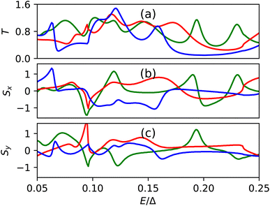Fig. 3 Variation of (a) conductance (T) and the spin response, (b) S_x, and (c) S_y functions on the 6th magnetic site. Red, blue and green lines correspond three different magnetic configurations.

One can readily see from Fig. 3 that the responses are highly nonlinear in nature within our chosen energy window and completely uncorrelated for different magnetic configurations. For simplicity we consider collinear magnetism (m_i = ±1) while the energy is kept as a continuous variable. The formalism is also applicable for non-collinear magnetism; however it would expand the input parameter space since each magnetic moment has to be described using three components.

2.3 Classical and quantum machine learning

Any machine learning approach consists of two steps – training and testing. For training one has to consider a large number of data sets where both inputs and outputs are known. For testing we use new input values and predict the output. In our case, we consider 17 input parameters. The first 16 are the magnetization directions of the 16 magnetic sites denoted by integers (1 for ↑ spin and −1 for ↓ spin) and the 17th input is the energy at which we calculate the desired output and is a floating number between 0.0 and 0.2. For outputs we consider conductance of the system and the x and y components of non-equilibrium spin density at each of the 16 magnetic sites. The sample data are produced using the non-equilibrium Green's function method which is computationally quite demanding since it requires quantum mechanical description of the complete system including the non-magnetic sites and the electrodes. Depending on the method and observable of interest these calculations can scale as n³ or at best n where n is the dimension of the Hamiltonian matrix of the complete system. Here we choose a system large enough to demonstrate significant non-linearity in the physical observables. The machine learning approach we present here, however, is not restricted by the dimensions of the physical system.

First we compare the performance of different classification algorithms, e.g., logistic regression,³⁹k-nearest neighbors (KNN),⁴⁰ random forest,⁴¹ support vector machine (SVM),⁴²etc. to train the models. Then, we use the trained models on the respective test samples and obtain the outputs. Among all the above classifiers the random forest algorithm performs the best and therefore we consider random forest throughout this paper. For comparison we also choose different regression models, e.g., the Theil-Sen regressor,^43,44 RANSAC (random sample consensus) regressor,⁴⁵ and SGD (stochastic gradient descent) regressor⁴⁶ for the data analysis, but the regressors perform much worse than the classifiers.

For a complex inhomogeneous multilevel nano-devices the number of governing parameters can be exponentially large which can be challenging for a classical computer. For such cases quantum machine learning algorithms can provide an efficient alternative. One of the most popular quantum classifiers is the quantum support vector machine (QSVM),^47,48 which is a quantized version of the classical SVM.⁴² It performs the SVM algorithm using quantum computers. It calculates the kernel-matrix using the quantum algorithm for the inner product on quantum random access memory (QRAM)⁴⁹ and performs the classification of query data using trained qubits with a quantum algorithm. The overall complexity of the quantum SVM is , whereas classical complexity of the SVM is , where N is the dimension of the feature space and M is the number of training vectors. The complexity of the random forest algorithm (the best performing algorithm for our dataset) is , where M, N, and T are the number of instances in the training data, the number of attributes, and the number of trees respectively. Therefore, the QSVM model for the solution of classification and prediction offers an exponential speed-up over its classical counterpart. Beside the QSVM, an alternate class of quantum classification algorithm is introduced,^50,51 called the variational quantum classifier (VQC). This NISQ-friendly algorithm operates through using a variational quantum circuit to classify a training set in direct analogy to conventional SVMs.

2.4 Regression vs. classification

Conventionally, physical observables are calculated within the linear response regime where linear regression can provide reasonable accuracy.³⁰ However, for a highly non-linear response, such as that shown in Fig. 3, applicability of regression becomes quite non-trivial. To increase the accuracy and efficiency of the learning process, here we adopt an alternative approach. First we discretize the output within small blocks and assign a class to each block (Fig.  4). To demonstrate this we consider the transmission spectrum corresponding to the green line in Fig. 3.

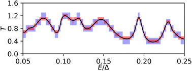Fig. 4 Discretization of the continuous output. Blue and red boxes correspond to block heights of 0.2 and 0.1.

For a block height δ, the class of an output y is defined as , where Round[] represents rounding off to the nearest integer. In this way a trained network can predict a class for an unknown set of input parameters, from which one can retrieve the actual value y as . Therefore δ corresponds to the intrinsic uncertainty of the discretization. A larger value of δ would reduce the number of classes and therefore increase the accuracy of the prediction; however the predicted value can significantly differ from the actual value due to the uncertainty posed by δ and therefore increase the overall error. A small value of δ on the other hand can reduce the uncertainty; however it would increase the number of classes significantly and therefore may pose a computational challenge for the learning algorithm.

3 Results and discussion

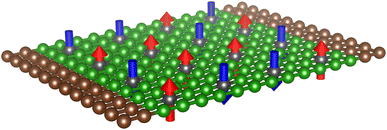
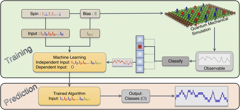
As mentioned in Sec. 2, we consider a scattering region with 16 magnetic sites where the magnetizations can either point up or down (Fig. 1). This gives a total of 2¹⁶ different configurations. For each of these configurations, one can calculate the transmission at any arbitrary energy which we choose between 0 and 0.2Δ. We are therefore dealing with a 17 dimensional feature space with mixed input variables where the first 16 inputs are either −1 (for spin ↓) or 1 (for spin ↑) and the 17th input is a floating number between 0 and 200 denoting the energy. For our study, we consider a set of 10⁵ random input configurations and calculate the corresponding transmission values and both the x and y components of spin response functions on all 16 magnetic sites. The theoretical workflow is outlined in Fig. 5.

Fig. 5 Schematic representation of the data analysis.

It is worth mentioning that state-of-the art AI models can handle billions of parameters which requires months of training. However, for most physical problems the challenge is to express the physical observable as a function of the minimum number of parameters. Besides, experimentally one can obtain only a few features of a system and therefore for practical use one requires a method which can predict a highly nonlinear outcome from fewer input parameters which is the main objective of this work.

3.1 Success rate vs. accuracy with number of classes

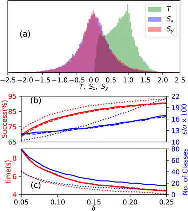
The samples are randomly split into 9 × 10⁴ training data and 10⁴ testing data and then we conduct 50 different train-test cycles. The number of classes depends on the choice of the parameter δ. As discussed earlier, reducing δ can decrease the error; however it also increases the number of classes and therefore reduces the accuracy. Unless otherwise mentioned, we keep δ = 0.1 which provides good balance between accuracy and error. Due to the highly non-linear nature of the system, there are few high values of the physical observable (Fig. 6a) which can significantly increase the total number of classes where the higher classes would have insignificant population. This in turn can reduce the performance of the learning algorithm. To avoid this scenario we set an upper cutoff of 2 for T and S_x,y, which means any value greater/less than ±2 is considered ±2. The performance of prediction is characterized in terms of the success rate and accuracy, where the accuracy is defined as the ratio of the root mean square error (RMSE) ε of the prediction to the standard deviation σ of the training data (Fig. 6b). This scales down the change in accuracy due to the variation of distribution of output classes. We try several training algorithms such as KNeighbors, decision tree and random forest. Among these methods random forest shows better performance within a reasonable execution time (Fig. 6c), and therefore we use random forest throughout the rest of the study.

Fig. 6 Comparison of predictions for T, S_x, and S_y with respect to the discretization parameter δ. (a) Distribution of the values of T, S_x, and S_y for δ = 0.1. (b) Success rate of the prediction (red) and accuracy (ε/σ) (blue), where the solid, dashed, and dotted lines correspond to S_x, S_y, and T respectively. (c) Time consumption (red) and number of classes (blue) for S_x (solid), S_y (dashed) and T (dotted).

Note that unlike T, S_x,y can have both positive and negative values and therefore for the same value of δ it results in twice the number of classes for S_x,y compared to T (Fig. 6c). This enhancement of classes along with the localization of spin density, as shown by the peaks causes a slight reduction in the success rate and detection efficiency compared to that of T (Fig. 6b).

3.2 Prediction of transmission and spin response functions

As one can see from Fig. 2, the band structure and therefore the physical properties depend crucially on the choice of parameter. This in turn affects the distribution of the outputs and therefore the prediction itself. To demonstrate this we consider six different values of the parameter t_R, as shown in Fig. 2 and calculate 10⁵ sample points by randomly varying the onsite magnetization m_i and energy where the energy values are kept within [0, 0.2Δ]. Training is performed with randomly chosen 9 × 10⁴ data and the testing is performed on the rest of the 10⁴ data points using the random forest algorithm. The success and accuracy are calculated by averaging over 50 different train-test cycles. The 50-fold cross validation ensures that the model is free from overfitting.

From Table 1, one can see that the quality of prediction gets better for higher values of t_R. This is because for smaller values of t_R, the entire energy range (green region in Fig. 2) is not spanned by bands and therefore for a large number of input data the output remains 0. As we increase the value of t_R the selected energy range is covered with bands resulting in more ordered finite outputs. Physically, an increased Rashba parameter can suppress scattering therefore reduce the fluctuation of the transmission which results in a better prediction. For the rest of the paper we consider t_R = 0.1Δ. To demonstrate the quality of the prediction we consider the three configurations shown in Fig.  3a and evaluate the transmission coefficient on uniformly spaced energy values (Fig. 7a).

Table 1 Qualitative variation of the prediction with respect to the Rashba parameter t_R

t R/Δ	Success (%)	ε/σ	N class	t Train (s)	t Test (s)
0.00	85.90	13.94	25	5.06	0.20
0.05	84.46	12.41	22	5.15	0.20
0.10	84.33	12.28	21	5.26	0.21
0.15	87.50	10.63	22	4.97	0.20
0.20	89.20	11.80	19	4.80	0.19
0.25	90.46	9.82	20	4.78	0.19

---

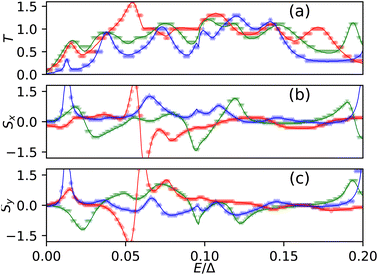Fig. 7 Comparison of the predicted values against the actual values of (a) T, (b) S_x, and (c) S_y for three different configurations. The symbols show the predicted values and the lines show the numerically calculated values (Fig. 3).

In our test system we have 16 magnetic centers where we calculate the spin response functions. For this study we keep t_R = 0.1Δ and train with the random forest algorithm. For brevity, we show S_x and S_y only at the 6th magnetic site which has been shown for the three specific configurations in Fig.  3. To demonstrate the quality of our prediction we also consider three particular configurations (Fig. 3b and c) and compared the predicted values against the calculated values (Fig. 7b and c).

3.3 Application of quantum classifiers

Finally we demonstrate the feasibility of quantum machine learning (QML) for our problem. Due to the limitation of resources it is not possible to handle a large number of input parameters or classes in this case. Therefore, we consider a particular magnetic configuration and choose the Rashba parameter (t_R) and the transmission energy (E) as the two components of the input variable and the sign of non-equilibrium S_x,y on each site as the two output classes. Physically speaking the sign of S_x and S_y determines the switching direction and direction of precession of the magnetic moments. We generate 1000 random input points in this two-dimensional t_R − E space and evaluate the sign of S_x,y for each of the 16 magnetic sites. A sample dataset is presented in Fig. 8.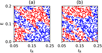

Fig. 8 A sample dataset with two features and two classes. Blue and red dots show the 0 and 1 classes for (a) S⁶_x and (b) S⁶_y.

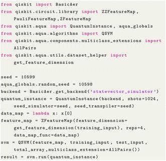
We divide each dataset into two parts, namely, training data (900 data points) and testing data (100 data points). We implement the classical SVM using Scikit-learn,⁵² and QSVM with Qiskit⁵³ from IBMQ, using different feature maps (e.g., ZFeatureMap, ZZFeatureMap, etc.), to classify the data. We repeat the above procedure with all 16 datasets and summarize the results in Table 2. For brevity we show S_x,y for only the first 8 sites.

Table 2 Comparing the testing accuracies between different classical and quantum classifiers for the S_x and S_y for the first 8 magnetic sites. In the above table RBF, Lin, and Poly represent the RBF, linear, and polynomial kernels used in the SVM algorithm

Quantity	QSVM	SVM (RBF)	SVM (Lin)	SVM (Poly)
S ^1 x	83%	81%	58%	58%
S ^1 y	78%	77%	71%	71%
S ^2 x	83%	80%	79%	79%
S ^2 y	90%	92%	93%	93%
S ^3 x	77%	69%	54%	64%
S ^3 y	79%	75%	62%	71%
S ^4 x	85%	76%	71%	68%
S ^5 y	82%	79%	82%	78%
S ^5 x	82%	78%	73%	73%
S ^5 y	84%	84%	51%	64%
S ^6 x	83%	89%	64%	67%
S ^6 y	76%	75%	63%	69%
S ^7 x	75%	75%	58%	70%
S ^7 y	80%	73%	63%	70%
S ^8 x	78%	81%	66%	68%
S ^8 y	74%	75%	60%	64%

---

From Table 2, we see that the quantum classifier is performing better than its classical counterpart in many cases. Although, the main advantage of QML over classical ML is in the runtime (see Sec.  2.3), for a significantly larger data size and configuration space QML will be the only feasible option. Therefore, with the availability of sufficient quantum computing resources this approach will be very useful to analyze large solid state and molecular devices as well.

4 Conclusion

In this article, we demonstrate the applicability of different classical and quantum machine learning approaches for spintronics. We show how one can achieve a significantly improved performance by converting the conventional regression problem into a discretized classification problem. Our approach allows us to obtain a high level of accuracy even for a strongly nonlinear regime. We further demonstrate the applicability of quantum machine learning which performs quite well for our small feature space. Considering the scalability of quantum machine learning algorithms over their classical counter parts (see Sec. 2.3) this will significantly enhance the performance for a larger configuration space and data size; in fact QML will be the only viable option in that regime. Our method is quite generic and therefore is equally applicable to a large class of systems, especially, for molecular devices. In these devices one can use additional charge or orbital degrees of freedom along with the spin to control different physical observables. In the case of a complex realistic device one can obtain the training data with state-of-the-art ab initio calculations or directly from an experiment. Due to its inherent ability to handle high orders of non-linearity, our approach can be used with both simulated as well as experimental data. Our work thus opens new possibilities to study a large variety of physical systems and their physical properties with machine learning.

Relevant codes for data analysis and machine learning

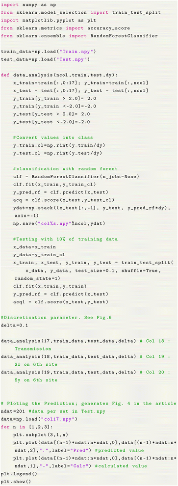
The supporting data and codes for this study are available in the following GitHub repository: https://github.com/jbghosh/ML_QML_Spintronics. Classical ML is implemented in RF_fit.ipynb. Train.npy contains 10⁵ training data and Test.npy contains testing data for the three specific configurations used in Fig. 3, where each configuration has 201 uniformly spaced energy values. The data structure is as follows: the first 16 columns describe the magnetic configurations of the 16 magnetic sites. The 17th column represents the energy at which the desired output is computed. The 18th column denotes the transmission. The 19th and 20th columns are the spin-components for the 6th magnetic site respectively. A sample code for classical data analysis is described below.

For quantum machine learning with the QSVM we prepare the sample training and test inputs from TrainQ.npy. The first 2 columns of the dataset represent the Rashba parameter (t_R) and the transmission energy (E) respectively. The third column onward represents different output-columns and the sign of non-equilibrium S_x,y on each site as the two output classes. In the following we present a sample code for implementing the QSVM described in Section 3.3.

Data availability

The data and codes that support the findings of this study are available in the following GitHub repository: https://github.com/jbghosh/ML_QML_Spintronics.

Conflicts of interest

There are no conflicts to declare.

References

1. S. Russell, P. Norvig and J. Canny, Artificial Intelligence: A Modern Approach, Prentice Hall/Pearson Education, 2003.
2. N. Artrith, K. T. Butler, F.-X. Coudert, S. Han, O. Isayev, A. Jain and A. Walsh, Nat. Chem., 2021, 13, 505–508.
3. K. T. Schütt, M. Gastegger, A. Tkatchenko, K.-R. Müller and R. J. Maurer, Nat. Commun., 2019, 10, 1–10.
4. J. P. Janet and H. J. Kulik, Machine Learning in Chemistry, American Chemical Society, 2020.
5. C. Pang, F. Prabhakara, A. El-abiad and A. Koivo, IEEE Trans. Power Appar. Syst., 1974, 93, 969–976.
6. H. Ghoddusi, G. G. Creamer and N. Rafizadeh, Energy Economics, 2019, 81, 709–727.
7. Y. Xin, L. Kong, Z. Liu, Y. Chen, Y. Li, H. Zhu, M. Gao, H. Hou and C. Wang, IEEE Access, 2018, 6, 35365–35381.
8. S. Omar, A. Ngadi and H. H. Jebur, Int. J. Comput. Appl., 2013, 79, 33–41.
9. J. Vamathevan, D. Clark, P. Czodrowski, I. Dunham, E. Ferran, G. Lee, B. Li, A. Madabhushi, P. Shah, M. Spitzer and S. Zhao, Nat. Rev. Drug Discovery, 2019, 18, 463–477.
10. M. A. Nielsen and I. Chuang, Quantum computation and quantum information, 2002.
11. M. Schuld, I. Sinayskiy and F. Petruccione, Contemp. Phys., 2014, 56, 172–185.
12. J. Biamonte, P. Wittek, N. Pancotti, P. Rebentrost, N. Wiebe and S. Lloyd, Nature, 2017, 549, 195–202.
13. A. Sakhnenko, C. O'Meara, K. Ghosh, C. B. Mendl, G. Cortiana and J. Bernabé-Moreno, Quantum Mach. Intell., 2022, 4, 1–17.
14. S. Woerner and D. J. Egger, npj Quantum Inf., 2019, 5, 1–8.
15. B. P. Lanyon, J. D. Whitfield, G. G. Gillett, M. E. Goggin, M. P. Almeida, I. Kassal, J. D. Biamonte, M. Mohseni, B. J. Powell, M. Barbieri, A. Aspuru-Guzik and A. G. White, Nat. Chem., 2010, 2, 106–111.
16. Y. Cao, J. Romero and J. P. Olson, et al. , Chem. Rev., 2019, 119, 10856–10915.
17. A. Kandala, A. Mezzacapo, K. Temme, M. Takita, M. Brink, J. M. Chow and J. M. Gambetta, Nature, 2017, 549, 242–246.
18. R. Eskandarpour, K. Ghosh, A. Khodaei, A. Paaso and L. Zhang, IEEE Access, 2020, 8, 188993–189002.
19. R. Eskandarpour, K. Ghosh, A. Khodaei and A. Paaso, arXiv, 2021, preprint, arXiv:2106.12032[quant-ph],  DOI:10.48550/arXiv.2106.12032.
20. V. Giovannetti, S. Lloyd and L. Maccone, Science, 2004, 306, 1330–1336.
21. A. Wichert, Principles of quantum artificial intelligence: quantum problem solving and machine learning, World Scientific, 2020.
22. E. Bedolla, L. C. Padierna and R. Castañeda-Priego, J. Phys.: Condens. Matter, 2020, 33, 053001.
23. R. Xia and S. Kais, Nat. Commun., 2018, 9, 1–6.
24. J. Weber, W. Koehl, J. Varley, A. Janotti, B. Buckley, C. Van de Walle and D. D. Awschalom, Proc. Natl. Acad. Sci. U. S. A., 2010, 107, 8513–8518.
25. A. Smith, M. Kim, F. Pollmann and J. Knolle, npj Quantum Inf., 2019, 5, 1–13.
26. A. Chandrasekaran, D. Kamal, R. Batra, C. Kim, L. Chen and R. Ramprasad, npj Comput. Mater., 2019, 5, 1–7.
27. J. Westermayr, M. Gastegger, K. T. Schütt and R. J. Maurer, J. Chem. Phys., 2021, 154, 230903.
28. L. Fiedler, K. Shah, M. Bussmann and A. Cangi, Phys. Rev. Mater., 2022, 6, 040301.
29. A. Lopez-Bezanilla and O. A. von Lilienfeld, Phys. Rev. B: Condens. Matter Mater. Phys., 2014, 89, 235411.
30. T. Wu and J. Guo, IEEE Trans. Electron Devices, 2020, 67, 5229–5235.
31. A. Manchon and S. Zhang, Phys. Rev. B: Condens. Matter Mater. Phys., 2008, 78, 212405.
32. A. Manchon and S. Zhang, Phys. Rev. B: Condens. Matter Mater. Phys., 2009, 79, 094422.
33. S. Ghosh and A. Manchon, Phys. Rev. B, 2017, 95, 035422.
34. S. Ghosh and A. Manchon, Phys. Rev. B, 2018, 97, 134402.
35. S. Ghosh and A. Manchon, Phys. Rev. B, 2019, 100, 014412.
36. B. K. Nikolić, S. Souma, L. P. Zârbo and J. Sinova, Phys. Rev. Lett., 2005, 95, 046601.
37. B. K. Nikolić, K. Dolui, M. D. Petrović, P. Plecháč, T. Markussen and K. Stokbro, Handb. Mater. Model., Springer International Publishing, 2018, pp. 1–35.
38. C. W. Groth, M. Wimmer, A. R. Akhmerov and X. Waintal, New J. Phys., 2014, 16, 063065.
39. D. G. Kleinbaum and M. Klein, Logistic regression, Springer, 2002.
40. O. Kramer, in K-Nearest Neighbors, Springer Berlin Heidelberg, Berlin, Heidelberg, 2013, pp. 13–23.
41. L. Breiman, Mach. Learn., 2001, 45, 5–32.
42. C. Cortes and V. Vapnik, Mach. Learn., 1995, 20, 273–297.
43. H. Theil, Proc. K. Ned. Akad. Wet., Ser. A: Math. Sci., 1950, 12, 173.
44. P. K. Sen, J. Am. Stat. Assoc., 1968, 63, 1379–1389.
45. M. A. Fischler and R. C. Bolles, Commun. ACM, 1981, 24, 381–395.
46. L. Bottou and O. Bousquet, Advances in Neural Information Processing Systems, 2007.
47. J. Pan, Y. Cao, X. Yao, Z. Li, C. Ju, H. Chen, X. Peng, S. Kais and J. Du, Phys. Rev. A: At., Mol., Opt. Phys., 2014, 89, 022313.
48. Z. Li, X. Liu, N. Xu and J. Du, Phys. Rev. Lett., 2015, 114, 140504.
49. V. Giovannetti, S. Lloyd and L. Maccone, Phys. Rev. Lett., 2008, 100, 160501.
50. K. Mitarai, M. Negoro, M. Kitagawa and K. Fujii, Phys. Rev. A, 2018, 98, 032309.
51. V. Havlíček, A. D. Córcoles, K. Temme, A. W. Harrow, A. Kandala, J. M. Chow and J. M. Gambetta, Nature, 2019, 567, 209–212.
52. F. Pedregosa, G. Varoquaux, A. Gramfort, V. Michel, B. Thirion, O. Grisel, M. Blondel, P. Prettenhofer, R. Weiss and V. Dubourg, et al. , J. Mach. Learn. Res., 2011, 12, 2825–2830.
53. G. Aleksandrowicz, et al., Qiskit: An Open-source Framework for Quantum Computing, 2021.

---