Development of a novel wavelength selection method for the trace determination of chlorpyrifos on Au@Ag NPs substrate coupled surface-enhanced Raman spectroscopy

Abstract

A novel wavelength selection method, namely interval combination population analysis-minimal redundancy maximal relevance (ICPA-mRMR), was employed for the trace level detection of chlorpyrifos (CPS) coupled surface-enhanced Raman spectroscopy (SERS). Herein, a highly sensitive SERS enhancement substrate, Au@Ag nanoparticles (NPs), was synthesized possessing strong enhancement of Raman signals for CPS quantification (enhancement factor: 2.5 × 10⁶). Compared with other established methods such as partial least squares (PLS), synergy interval partial least squares-genetic algorithm (siPLS-GA) and competitive adaptive reweighted sampling-partial least squares (CARS-PLS), ICPA-mRMR yielded the best results with higher correlation coefficients (R_c = 0.9917, R_P = 0.9895), ratios of performance to deviation (RPD = 6.8797), and lower root mean square errors (RMSEC = 0.1998, RMSEP = 0.2271). The proposed method was employed for the determination of trace level CPS in tea samples, and the recovery percentages were in the range 90%–108%. Meanwhile, this method was validated using a standard GC-MS method indicating no significant difference (P > 0.05). The proposed methodology offers a rapid, sensitive and powerful analytical platform for the detection of pesticide residues in food.

---

1. Introduction

In modern agricultural practices, pesticides play a crucial role in protecting crops and seeds. A conservative estimate is that if pesticides were not used, one-third of crops around the world would be damaged by pests and diseases during growth, harvest or storage.¹ Nevertheless, pesticides are a double-edged sword, and their unsafe use in agricultural production might lead to the problems of accumulation and health hazards. From the perspective of the nature of pesticides, they may pose risks to threaten human and aquatic life. For instance, chlorpyrifos (CPS) as an organophosphate pesticide is used to control pests on rice, wheat, cotton, fruits, and tea plants by inhibiting acetylcholinesterases of pests.² Thus it might impact the nerve impulses and leads to a variety of conditions like abnormal excitation, spasms, and even to death in extreme cases. The maximum allowed limit, known as tolerance, for CPS in food or water as recommended by the WHO is set to 0.1 part per million (ppm) in an attempt to improve the food safety campaigns for the detection of toxic contaminants and/or residues in foodstuffs.³

Over the past decades, many routine methods, such as high-performance liquid chromatography (HPLC), liquid chromatography-mass spectrometry (LC-MS), fluorescence spectroscopy, gas chromatography-mass spectrometry (GC-MS) and enzyme-linked immunosorbent assay (ELISA) were well established for the detection of pesticide residues.^4–8 Some of the above mentioned methods are highly reliable and sensitive, yet possess disadvantages like complicated sample preparation steps, high instrument cost, large volumes of expensive and toxic solvents, and expertise in operations. Therefore, developing a simple, rapid, inexpensive, selective and highly reliable detection strategy for pesticide residues in complicated matrices was highly needful.

Raman spectroscopy as a vibrational spectroscopic technique which relies on a scattering effect of molecules and records a loss of energy in incident light has been employed in the fields of food safety and bioanalysis.^9,10 Raman spectra are information derived from molecular vibrations and rotations, and can be applied to study molecular structure and molecular fingerprint specificity. However, the weak signal of Raman spectroscopy restricts its applications in the field of trace level detection. Surface-enhanced Raman spectroscopy (SERS) is among the widely employed and highly sensitive analytical techniques in the fields of food science, biosensors and medical diagnostics, which makes up the drawback of Raman spectroscopy.^11–17 In SERS measurements, the target molecule adsorbed on and/or at the vicinity of rough noble metal NPs (usually gold, silver or copper NPs) generates a strong enhancement of the Raman signal. According to a previous report,¹⁸ the enhancement factor (EF) of SERS enhancement substrate might reach up to the order of 10⁶–10¹⁴. However, the spectra collected from SERS suffer from the curse of dimensionality; this means that the number of samples is much smaller than the number of variables, which results in a great challenge in the construction of a parsimonious calibration model. Therefore, wavelength selection is a critical step in multivariate calibration.

The objective of wavelength selection is to retain informative variables and remove uninformative or interfering variables, thereby improving the prediction performance of calibration models. According to different selection strategies, these wavelength selection methods can be divided into two categories: individual wavelength selection and wavelength intervals selection. The individual wavelength selection methods include uninformative variable elimination (UVE),¹⁹ Monte Carlo based UVE (MC-UVE),²⁰ competitive adaptive reweighted sampling (CARS),^21,22 genetic algorithm (GA),²³ stepwise selection²⁴ and successive projection algorithm (SPA).^25,26 Based on various kinds of criteria such as correlation coefficient, t-statistics and the mean squared error in prediction (MSEP), the importance of individual wavelengths is calculated. However, individual wavelength selection methods are neither intuitive nor easy to interpret the selected wavelengths corresponding to the chemical properties of interest. Moreover, individual wavelengths are not robust to noise. Considering the fact that the vibrational and rotational spectra have continuous features of spectral bands, it is reasonable and interpretable to select wavelength intervals instead of individual wavelengths. The wavelength intervals selection methods include interval partial least squares (iPLS),²⁷ backward iPLS (biPLS),²⁸ synergy iPLS (siPLS),²⁹ moving window PLS (MWPLS)³⁰ and interval random frog (iRF).³¹ Nevertheless, it is important to emphasize that wavelength interval selection methods usually face the problem of retaining uninformative or interfering variables in selected spectral intervals, which would deteriorate the prediction performance of calibration models. Hence, wavelength intervals selection methods together with redundant information removing methods might serve as a promising combination for improving the prediction performance of calibration models.

Herein, the current study aimed to develop a rapid, low-cost, and highly sensitive method for quantification of CPS residues using SERS coupled to a novel wavelength selection method. For obtaining the SERS spectra of CPS residues, Au@Ag NPs were synthesized for the enhancement of Raman signals. In order to reduce the dimensionality of SERS spectra datasets and provide a faster and more cost-effective calibration model, a novel wavelength selection method called interval combination population analysis-minimal redundancy maximal relevance (ICPA-mRMR) was proposed for the first time. The outcome of this study is expected to provide a powerful strategy for the quantification of CPS residues in food.

2. Experimental and algorithm

2.1 Chemicals and reagents

All the reagents were of analytical grade and used without further purification. Sodium citrate (Na₃C₆H₅O₇·2H₂O), chloroauric acid (HAuCl₄·4H₂O), silver nitrate (AgNO₃), ascorbic acid (C₆H₈O₆), and methanol (CH₃OH) were purchased from Sinopharm Chemical Reagent Co., Ltd. (Shanghai, China). CPS (C₉H₁₁Cl₃NO₃PS) was purchased from Shanghai Pesticide Research Institute (Shanghai, China). Ultrapure water (18.2 MΩ cm) was produced by the Smart-N2 UV water purification system (Heal Force Bio-meditech Holdings Limited, Shanghai, China).

2.2 Preparation of Au@Ag NPs

Referring to the a previous study,³² uniform Au@Ag NPs were synthesized in aqueous solution via seed growth through consecutive two-step reactions. Firstly, Au cores with a size of 30 nm were prepared using the chemical reduction of chloroauric acid with sodium citrate. Secondly, Ag shells with a size of 7 nm were grown on the surface of the Au cores using the chemical reduction of silver nitrate with ascorbic acid. The obvious color change from wine red to orange was correlated with the formation of Au@Ag NPs (detailed procedures are shown in ESI†).

2.3 Preparation of CPS standard solutions

An accurate weight (5.259 × 10⁻³ g) of CPS powder was dissolved in 50 mL of ultrapure water/methanol (70 : 30, v/v) to prepare a standard stock solution (3.0 × 10⁻⁴ mol L⁻¹). More diluted standard solutions were prepared from the stock (1.0 × 10⁻⁴, 7.0 × 10⁻⁵, 5.0 × 10⁻⁵, 3.0 × 10⁻⁵, 7.0 × 10⁻⁶, 5.0 × 10⁻⁶, 3.0 × 10⁻⁶, 1.0 × 10⁻⁶, 7.0 × 10⁻⁷, 5.0 × 10⁻⁷, 3.0 × 10⁻⁷, 7.0 × 10⁻⁸, 5.0 × 10⁻⁸, 3.0 × 10⁻⁸, 1.0 × 10⁻⁸, 7.0 × 10⁻⁹, 5.0 × 10⁻⁹, and 3.0 × 10⁻⁹ mol L⁻¹). Finally, 10 CPS standard solution samples were prepared for each concentration gradient (19 concentration gradients: 3.0 × 10⁻⁴–3.0 × 10⁻⁹ mol L⁻¹), thus 190 CPS standard solution samples were obtained.

2.4 SERS measurements and spectra data preprocessing

For SERS measurements, the analyte was prepared by evenly mixing 20 μL of synthesized Au@Ag NPs and 180 μL of CPS standard solution, and then 10 μL of the mixture was deposited on a quartz plate. The SERS spectra were collected using a micro-Raman system (SPL-Raman-785, SPL Photonics Co., Ltd, Hangzhou, China) equipped with a 256 × 1024 pixel CCD detector, a 785 nm laser excitation source, and a microscopic module. The laser beam focused on the sample was approximately 50 mW. Each spectrum was the average of 3 scans with an acquisition time of 2 s. Five spectra from different spots on the surface of the sample were collected and the average was calculated for data analysis. Ocean View 1.6.3 software was employed to obtain and display SERS spectra in the Raman shift range 200–2000 cm⁻¹ at a spectral resolution of 2 cm⁻¹.

In total, 190 SERS spectra of CPS standard solutions were collected (1 spectrum for a standard solution sample) and the spectra have been recorded from 560 to 1701 cm⁻¹ (587 wavelengths). Moreover, for the development of the calibration model, the CPS SERS spectra data were divided into a calibration set (19 × 6, 6 SERS spectra for each concentration) and a prediction set (19 × 4, the remaining 4 SERS spectra for each concentration). Prior to employing the SERS spectra, standard normal variate transformation (SNV) and Savitzky–Golay smoothing were applied to eliminate baseline drift and random noise.

2.5 The theory of ICPA

As a wavelength intervals selection method, ICPA is proposed to search the optimal intervals subset using root mean square error of cross-validation (RMSECV) as the objective function through random combination of spectral intervals. The SERS spectra data matrix X contains N samples in rows and p wavelengths in columns, and y, of size N × 1, denotes the measured property of interest. The main approaches of ICPA are illustrated as follows:

Division of intervals: Considering the calculation cost and the width of chemical bands, an interval width w of 5–20 spectral wavelengths should be set. Meanwhile, the continuity of spectra was taken into account, so the overlapping intervals were obtained. In this study, the interval width w was set as 20 wavelengths, P (p − w + 1) intervals that contained all possible intervals with 20 spectral wavelengths were obtained.

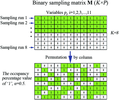
Binary matrix sampling (BMS): BMS was employed for generating a population of random combinations of intervals. In this study, a binary matrix M that only contains either ‘1’ or ‘0’ with dimensions K × P is generated. K denotes the number of sampling, and P is the number of intervals. The ‘1’ means the interval is sampled, while ‘0’ represents the opposite. In M, the number of ‘1’ is KPα and the number of ‘0’ is KP(1 − α) where α is the occupancy percentage value of ‘1’ in each column and it is inconstant due to the change of P intervals affected by each exponentially decreasing function (EDF) run. According to previous literature,³³α was set to /P in the first EDF run. In the final EDF run, α was set to (P/2)/P = (ω/2)/ω = 0.5, and P gradually decreases with EDF runs, and ultimately, ω intervals were left in the final run. In this work, α takes 500 values between /P and 0.5. The number of ‘1’ in each column is the same, which guarantees the same sampling chance for each interval. Subsequently, the M is permuted by column. The number of ‘1’ and ‘0’ in each column does not change. Each row of M determines which intervals are to be sampled for modeling, thus K sub-models which contain random combinations of intervals are obtained. This process is illustrated in Fig. 1 (just an example for illustration).

Fig. 1 The process of BMS.

Model population analysis (MPA): The core idea of MPA is to statistically analyze the performance of a large population of sub-models and extract useful information from the outputs of the sub-models. The RMSECV value of each sub-model obtained by 5-fold cross-validation is considered as an assessment criterion of model performance which means if the RMSECV value is lower, the prediction ability of the model is better. The distribution of RMSECV values for K sub-models obeys a normal distribution. The method is to choose σ as the ratio of best models of K sub-models and to count the frequency of each interval appearing in those best σ*K sub-models. If the frequency is higher, the interval becomes more important due to its larger contribution.

EDF: EDF was used to eliminate intervals with lower contributions. In this step, the runs of EDF are set to L, which means we will obtain an optimal interval combination highly correlated with y through L iterations. In the ith run of EDF, the ratio of remaining intervals r_i can be calculated using the following function:

r_i = e^−θi (1)

where θ is the constant parameter determined by the following conditions: (I) when i = 0, all the P intervals are used for modeling, so r₀ = 1; (II) in the Lth run, ω intervals are remaining, so the ratio r_L = ω/P. Combining two conditions, θ can be calculated as:where ln denotes the natural logarithm.

2.6 The theory of mRMR

In information theory,³⁴ the mutual information (MI) is used for measuring the degree of mutual dependence of two variables, which takes both linear and non-linear relevance into account. Given two random variables x and y, the MI is defined as:

I(x,y) = H(x) + H(y) − H(x,y) (3)

where H(·) is the information entropy of the variable, and H(x,y) is the joint information entropy of x and y. According to information entropy theory, H(x), H(y) and H(x,y) can be defined as:where p(x) and p(y) are margin probability density functions of x and y, respectively; p(x,y) is the joint probability density functions of x and y.

Then, eqn (3) can be written as:

If x and y are discrete variables, eqn (7) can be written as:

The MI method has been used for variable selection due to its excellent ability for relevance measurement, but the redundancy between the selected variables is serious. Thus, mRMR which takes both relevance and redundancy into account is proposed.³⁵

For instance, the maximal-relevance criterion maximizes the relevance of the variables in dataset S with target variable c, which can be defined as:

where |S| represents the number of variables in S, and I(x_i,c) represents the mutual information of x_i and c. Obviously, the variables selected by the maximal-relevance criterion have higher redundancy, thus a minimal-redundancy criterion might be introduced to minimize the redundancy. Minimal-redundancy criterion can be defined as:where I(x_i,x_j) represents the mutual information of selected variables x_i and x_j.

The combination of two constraints is called mRMR. We define the objective function Φ(D,R) which is the combination of D and R, and the following form is proposed for optimizing D and R simultaneously:

Max Φ(D,R), Φ(D,R) = D(S,c) − R(S) (11)

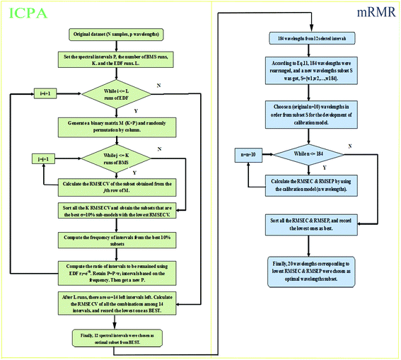
In this study, the optimal combination of intervals was selected by ICPA, but the selected spectral intervals might possess higher redundancy. Therefore, mRMR was employed and retained the most informative variables for the development of a calibration model. Fig. 2 shows the flowchart of ICPA-mRMR.

Fig. 2 The flowchart of ICPA-mRMR.

2.7 Brief introduction of the compared wavelength selection methods

To investigate the performance of ICPA-mRMR, three wavelength selection methods were performed for comparison. The following section briefly describes three methods:

(1) PLS; PLS retains all spectral wavelengths for the development of a calibration model. (2) siPLS-GA; siPLS-GA is a combination of siPLS and GA: firstly, siPLS selected the optimal combination of spectral intervals; secondly, GA is applied to eliminate the collinear wavelengths contained in the selected spectral intervals, which would improve the prediction performance of a calibration model. (3) CARS-PLS; CARS-PLS selects N subsets of wavelengths from N Monte Carlo sampling runs. Then, EDF is employed to perform enforced wavelengths selection. After that, adaptive reweighted sampling (ARS) is adopted to realize a competitive selection of wavelengths. Finally, cross-validation is applied to choose the optimal subset with the lowest RMSECV. The parameters of siPLS-GA and CARS-PLS are shown in Table 1.

Table 1 The parameters of siPLS-GA and CARS-PLS

siPLS-GA	The number of spectral intervals: 10
	The number of combined spectral intervals for each run: 4
	Population size: 30 chromosomes
	On average, 5 variables per chromosome in the original population
	Maximum number of variables selected in the same chromosome: 30
	Probability of cross-over: 50%
	Probability of mutation: 1%
	Number of runs: 100
	The amount of evaluations: 100
CARS-PLS	The number of Monte Carlo sampling runs: 500
	The ratio of Monte Carlo sampling: 90%

---

Root mean square error of calibration set (RMSEC), root mean square error of prediction set (RMSEP), correlation coefficient between reference values and predicted values of the calibration set (R_C), correlation coefficient between reference values and predicted values of the prediction set (R_P) and ratio of performance to deviation (RPD) were used to assess the performance of various wavelength selection methods. All algorithms were performed using Matlab R2010b (Mathworks, USA). The ICPA-mRMR was realized with home-made code which is available upon request.

3. Results and discussion

3.1 Characterizations of Au@Ag NPs and spectra analysis

The Au@Ag NPs with a 30 nm Au core and a 7 nm Ag shell were synthesized in aqueous solution using a seed growth method through consecutive two-step reactions. Morphological characterizations of Au@Ag NPs were performed using scanning electron microscopy (SEM) and transmission electron microscopy (TEM) to verify the shape, size and core–shell structure. Fig. 3(A) presents the SEM image of highly uniform Au@Ag NPs with an average particle size of ∼45 nm. The core–shell structure of Au@Ag NPs was clearly shown by the TEM image in Fig. 3(B). Fig. 3(C) shows the extinction visible spectrum of Au@Ag NPs with a wide range of plasmon resonances from 350 nm to 560 nm. The strong plasmonic absorption peaks at 410 nm and 500 nm were clearly observed, which were derived from the Ag shell and Au core, respectively. A satisfactory EF of magnitude 2.5 × 10⁶ was obtained for the Au@Ag NPs SERS substrate (calculated in ESI†). The EF reveals the applicability of the synthesized Au@Ag NPs SERS substrate for detecting trace level pesticide residues. Moreover, the suitability of the Au@Ag NPs SERS substrate was also confirmed by satisfactory reproducibility approximations (Table S1†).

Fig. 3 (A) SEM image of Au@Ag NPs. (B) TEM image of Au@Ag NPs with a 30 nm Au core and a 7 nm Ag shell. (C) Extinction visible spectrum of Au@Ag NPs.

Fig. 4 shows a representative SERS spectrum of CPS standard solution. The band assignments of major peaks for CPS SERS spectra are shown in Table 2.³⁶ CPS is a sulfur-containing pesticide with a P=S double bond which is responsible for improving the pest killing ability and pesticide effects. These sulfur-containing pesticide molecules usually exhibit strong adsorption abilities with some metal ions as new covalent bonds such as Ag–S, Au–S and Cu–S were formed.³⁷ This high affinity of sulfur-containing pesticides molecules towards metal ions might be exploited for trace level pesticide SERS detection.

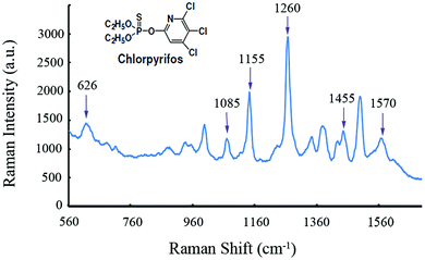Fig. 4 A representative SERS spectrum of 1.0 × 10⁻⁶ mol L⁻¹ CPS standard solution mixed with Au@Ag NPs.

Table 2 Band assignments of major peaks for CPS SERS spectra

Band (cm^−1)	Assignment
626	P=S stretch
1085	P–O–R stretch
1155	C–H deformation
1260	Ring mode
1455	C–H deformation
1570	Ring stretching mode

---

3.2 Optimization of parameters in ICPA

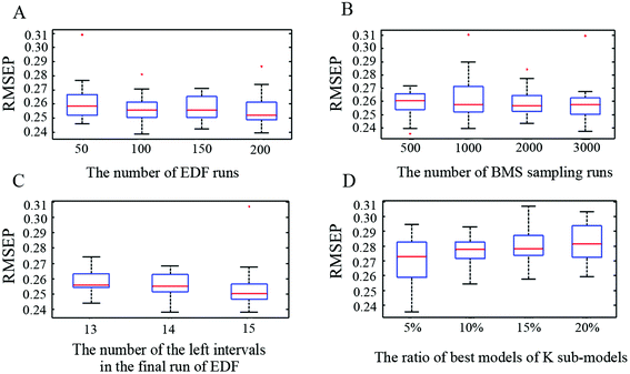
The performance of ICPA was influenced by four tuning parameters which were optimized by implementing 30 replicate runs of the ICPA algorithm on the CPS SERS spectra dataset. The RMSEP values were recorded for analysis and comparison. The four tuning parameters, as well as their optimizations, are shown as below:

(1) N, EDF runs. The number of EDF runs was optimized by investigating four cases including 50, 100, 150 and 200. By using boxplots, Fig. 5(A) shows the statistical results which revealed that the performance of ICPA is not significantly influenced by the number of EDF runs. But the result of 100 is slightly better than the results of 50, 150 and 200. Therefore, setting the number of N to 100 is appropriate.

Fig. 5 Boxplots of 30 RMSEP values for investigating the effect of (A) the number of EDF runs, N; (B) the number of BMS sampling runs, K; (C) the left intervals in the final run of EDF, ω; (D) the ratio of best models of K sub-models, σ.

(2) K, BMS sampling runs. The number of BMS sampling runs was optimized by investigating four cases including 500, 1000, 2000 and 3000. By using boxplots, Fig. 5(B) shows the statistical results which revealed that the number of BMS sampling runs does not have a significant influence on the performance of ICPA. Moreover, if K is larger, more calculation time is required for the computer. Therefore, setting the number of K to 500 is appropriate.

(3) ω, the number of the left intervals in the final run of EDF. It was optimized by investigating three cases including 13, 14 and 15. In addition, ω should be smaller than 16, because if ω equals 16, 65 535 (2¹⁶ − 1) combinations will not be computed in a common computer due to being out of memory. By using boxplots, Fig. 5(C) shows the statistical results which revealed that the result of 13 is slightly worse than the results of 14 and 15. Moreover, if the ω is larger, it will take more calculation time. Therefore, setting the number of ω to 14 is more suitable.

(4) σ, the ratio of best models of K sub-models. It was optimized by investigating four cases including 5%, 10%, 15% and 20%. In this study, K was optimized to 500, which means there are 25, 50, 75 and 100 best sub-models being selected, respectively. By using boxplots, as shown in Fig. 5(D), the statistical results revealed that 10% is better than 5%, 15% and 20%.

3.3 Quantification of CPS in standard solutions

For the quantification of CPS in standard solutions, wavelength selection methods including PLS, siPLS-GA, CARS-PLS, ICPA and ICPA-mRMR were applied respectively on SERS spectra to construct calibration models. In this work, the maximum number of latent variables was set to 10, and the optimal number of latent variables obtained by 5-fold cross-validation was used for the development of calibration models. The performance of various wavelength selection methods was evaluated by comparing the values of RMSEC, RMSEP, R_C, R_P, and RPD. The results of various wavelength selection methods are presented in Table 3.

Table 3 Comparison of various wavelength selection methods on the CPS SERS spectra dataset

Methods	Principal components	Number of variables	Calibration set		Prediction set		RPD^c
			RMSEC	R C ^a	RMSEP	R P ^b
a R C: correlation coefficient between reference values and predicted values of the calibration set. b R P: correlation coefficient between reference values and predicted values of the prediction set. c RPD: ratio of performance to deviation.
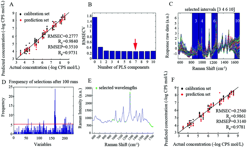
PLS	7	587	0.2777	0.9840	0.3510	0.9731	4.5062
siPLS-GA	6	30	0.2560	0.9861	0.3140	0.9781	4.9757
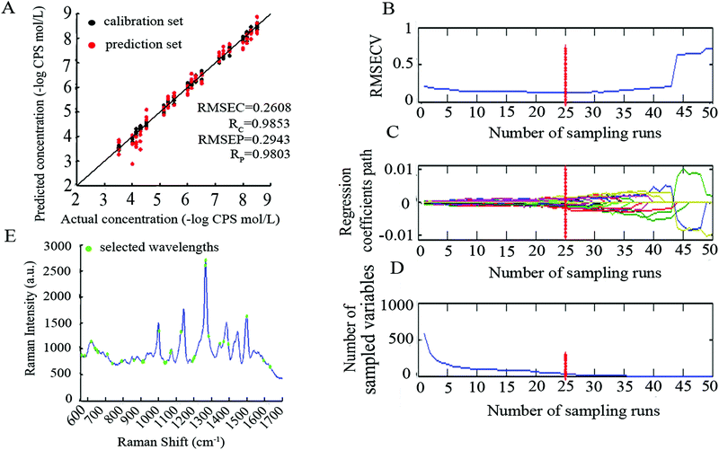
CARS-PLS	8	36	0.2608	0.9853	0.2943	0.9803	5.3088
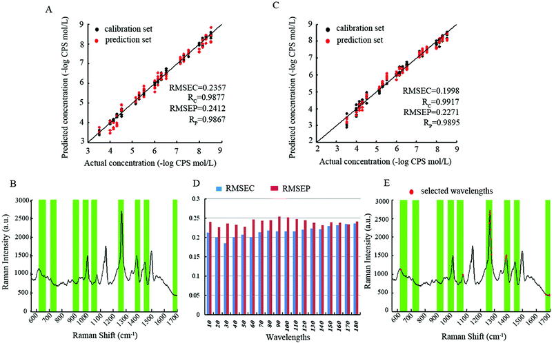
ICPA	10	184	0.2357	0.9877	0.2412	0.9867	6.0775
ICPA-mRMR	8	20	0.1998	0.9917	0.2271	0.9895	6.8797

---

3.3.1 Results of PLS built model. The PLS built model yielded RMSEC = 0.2777, R_C = 0.9840, RMSEP = 0.3510, R_P = 0.9731 and RPD = 4.5062. By comparison, it is quite clear that the results of the PLS built model are unsatisfactory, due to the retention of unnecessary wavelengths in the calibration model, adversely affecting the prediction performance. The linear regression plot of the calibration set and prediction set and the optimal principal components in the PLS built model are shown in Fig. 6(A) and (B), respectively.

Fig. 6 (A) A linear regression plot of the calibration set and the prediction set for the PLS built model; (B) the optimal principal components for the PLS built model; (C) the selected spectra intervals for the siPLS built model; (D) the frequency of variable selection after 100 runs by GA; (E) the distributions of selected wavelengths for the siPLS-GA built model; (F) a linear regression plot of the calibration set and the prediction set for the siPLS-GA built model.

3.3.2 Results of siPLS-GA built model. Firstly, siPLS split SERS spectra into 10 equal-width spectral intervals and combined 4 of them to explore their synergistic effects toward getting the lowest RMSECV. The siPLS models performances based on the variously combined selected intervals are summarized in Table S2.† As shown in Fig. 6(C), the optimal spectral intervals were selected with RMSECV = 0.26 and the four intervals (3, 4, 6 and 10) consist of 235 wavelengths that span among the spectral wavelength ranges of 823–1066 cm⁻¹, 1184–1294 cm⁻¹ and 1607–1700 cm⁻¹. Although these spectral intervals cover some Raman characteristic bands, some wavelengths in the selected intervals are still collinear, so further wavelength selection is necessary. Subsequently, based on siPLS selected intervals, the GA was employed to select 30 individual wavelengths for constructing the calibration model. The results of the siPLS-GA built model were: RMSEC = 0.2560, R_C = 0.9861, RMSEP = 0.3140, R_P = 0.9781 and RPD = 4.9757. The frequency and the distributions of the selected wavelengths are shown in Fig. 6(D) and (E) respectively. Some of the wavelengths selected by siPLS-GA like 1184, 1262, 1264, 1266, 1268, 1270, 1272 and 1274 cm⁻¹ are near to the Raman characteristic bands 1155 and 1260 cm⁻¹. The linear regression plot of the calibration set and the prediction set in the siPLS-GA built model is shown in Fig. 6(F).

3.3.3 Results of CARS-PLS built model. In this method, the CARS-PLS algorithm was applied to select 36 individual wavelengths for the development of the calibration model, yielding the following results: RMSEC = 0.2608, R_C = 0.9853, RMSEP = 0.2943, R_P = 0.9803 and RPD = 5.3088. The linear regression plot of the calibration set and the prediction set in the CARS-PLS built model is shown in Fig. 7(A). The change of RMSECV values for different numbers of sampling runs is shown in Fig. 7(B). The RMSECV values decreased for 1 to 25 sampling runs with the elimination of unnecessary wavelengths, with a subsequent increase in its value for 30 to 50 sampling runs on account of removing some informative wavelengths. The corresponding regression coefficients path and the number of sampled variables in different number of sampling runs are shown in Fig. 7(C) and (D) respectively. In general, the process of wavelength selection can be divided into two stages. Firstly, the wavelengths were removed quickly signifying a ‘fast selection’ stage; secondly, the wavelengths were removed gradually signifying a ‘refined selection’ stage. The distributions of the selected wavelengths are shown in Fig. 7(E). Among the CARS-PLS selected wavelengths, 620, 640, 1068, 1070, 1127, 1264 and 1266 cm⁻¹ are near to Raman characteristic bands 626, 1085, 1155 and 1260 cm⁻¹.

Fig. 7 (A) A linear regression plot of the calibration set and the prediction set for the CARS built model; the number of sampling runs versus (B) RMSECV, (C) regression coefficients path and (D) the number of sampled variables; (E) the distributions of selected wavelengths for the CARS built model.

3.3.4 Results of ICPA built model. ICPA was applied to select optimal spectral intervals to build the calibration model with the following results: RMSEC = 0.2357, R_C = 0.9877, RMSEP = 0.2412, R_P = 0.9867 and RPD = 6.0775. The linear regression plot of the calibration set and the prediction set in the ICPA built model is shown in Fig. 8(A). In this method, after 100 EDF runs, 14 significant spectral intervals were retained. The RMSECV values of all combinations of 14 spectral intervals were calculated, and the intervals combination with the lowest RMSECV was chosen. The optimal combination of intervals consists of 12 intervals (184 wavelengths) that span the spectral wavelength ranges of 622–669, 712–754, 889–929, 966–1005, 1031–1072, 1241–1279, 1374–1408, 1451–1484 and 1668–1700 cm⁻¹ (neighboring intervals were combined). These intervals cover all the Raman characteristic bands and the spectral intervals selected by ICPA are shown in Fig. 8(B).

Fig. 8 (A) A linear regression plot of the calibration set and the prediction set for the ICPA built model; (B) the selected spectral intervals for the ICPA built model; (C) a linear regression plot of the calibration set and the prediction set for the ICPA-mRMR built model; (D) the changes of RMSEC and RMSEP with different numbers of wavelengths; (E) the distributions of selected wavelengths for the ICPA-mRMR built model.

3.3.5 Results of ICPA-mRMR built model. Based on the spectral intervals selected by ICPA, the mRMR algorithm was applied to handle the redundancy. The calibration model built by ICPA-mRMR yielded the results: RMSEC = 0.1998, RMSEP = 0.2271, R_C = 0.9917, R_P = 0.9895 and RPD = 6.8797. According to the principle of mRMR, 184 wavelengths were rearranged by the criterion of wavelength importance (shown in Table S3†). Fig. 8(D) shows the changes of RMSEC and RMSEP with different numbers of wavelengths which are rearranged by mRMR inclusion in the calibration model. The values of RMSEC and RMSEP are high when the number of wavelengths is 10, because too few informative wavelengths are involved in the calibration model. The values of RMSEC and RMSEP decrease when increasing the number of wavelengths from 20 to 40. Subsequently, the values of RMSEC and RMSEP increase again with further increases in the number of wavelengths from 50 to 180, attributed to the inclusion of redundant wavelengths. Therefore, 20 wavelengths are optimally considered owing to the complexity and prediction performance of the calibration model. The distributions of the selected 20 wavelengths are shown in Fig. 8(E), and it implies good wavelength selection of the ICPA-mRMR. Some of the ICPA-mRMR selected wavelengths 626, 1071, 1262, 1264, 1266, 1268, 1269, 1271, 1273, 1275 and 1277 cm⁻¹ are near to Raman characteristic bands 626, 1085 and 1260 cm⁻¹. The linear regression plot of the calibration set and the prediction set in the ICPA-mRMR built model is shown in Fig. 8(C).

Comparing the results obtained from various methods, RPD values are all greater than 3, which indicates that all wavelength selection methods are capable of being combined with the SERS technique for the quantification of CPS in standard solutions. According to the values of RMSEC, R_C, RMSEP, R_P, and RPD, the prediction performances for various methods were of the order:

PLS < siPLS-GA < CARS-PLS < ICPA < ICPA-mRMR

The performance of the PLS method was lower compared to all other used wavelength selection methods, whereas the prediction results of the CARS-PLS built model were slightly better than that of siPLS-GA, attributed to the greater relevancy of CARS-PLS selected wavelengths to Raman characteristic bands. Compared with siPLS-GA and CARS-PLS, ICPA shows better prediction performance with respect to lower RMSEP, higher R_P and RPD. The reasons are: (1) the division of intervals, considering the continuous features of spectral bands, the spectral intervals divided by ICPA were overlapped, and on the contrary, the spectral intervals divided by siPLS were not overlapped, which would miss some more informative intervals; (2) EDF, in every EDF run, some intervals that made little contribution were eliminated, so with the decrease of RMSECV values, the intervals subset is gradually selected toward optimal; (3) BMS is a novel sampling method that gives all the intervals the same chance of being sampled which is superior to Monte Carlo sampling, and BMS makes different intervals combinations randomly for the development of sub-models; (4) MPA, the optimal intervals combination contained in a large population of sub-models can be extracted by MPA. Albeit the ICPA selected optimal spectral intervals with excellent prediction performance, the redundancy is still serious. Hence, the mRMR algorithm which takes both maximal relevance and minimal redundancy into account was employed. Based on the data obtained, the ICPA-mRMR built model shows the best prediction performance with fewest selected wavelengths.

3.4 Quantification of CPS in real samples

The applicability of the ICPA-mRMR wavelength selection method coupled with SERS for the determination of CPS was evaluated by spiking tea samples (Longjing tea) with different CPS concentration ranges (1.0 × 10⁻⁴–1.0 × 10⁻⁸ mol L⁻¹). In addition, the proposed methodology was validated using a standard GC-MS method. A series of pre-treatment procedures for tea samples were described in ESI.†Table 4 shows the values of recovery and relative standard deviation (RSD) obtained from the present method and GC-MS. It is evident that there was no significant difference between the values quantified by the present method and the standard GC-MS method, indicating the applicability and reliability of the proposed method for the quantification of CPS in real samples.

Table 4 The determination results of the proposed and standard GC-MS methods for CPS residues in spiked tea samples

Sample	Spiked concentration (mol L^−1)	Detection value (mol L^−1)		Recovery (%)		RSD (%)
		(Mean^a ± SD^b)
		Present method	GC-MS	Present method	GC-MS	Present method	GC-MS
a Mean: average value of 10 tests. b SD: standard deviation of 10 tests.
Tea	1.0 × 10^−4	0.93 × 10^−4 ± 0.03 × 10^−4	0.95 × 10^−4 ± 0.02 × 10^−4	93.00	95.00	3.23	2.11
	1.0 × 10^−5	0.97 × 10^−5 ± 0.05 × 10^−5	0.98 × 10^−5 ± 0.03 × 10^−5	97.00	98.00	5.15	3.06
	1.0 × 10^−6	1.05 × 10^−6 ± 0.06 × 10^−6	0.96 × 10^−6 ± 0.03 × 10^−6	105.00	96.00	5.71	3.13
	1.0 × 10^−7	0.90 × 10^−7 ± 0.07 × 10^−7	1.02 × 10^−7 ± 0.04 × 10^−7	90.00	102.00	7.78	3.92
	1.0 × 10^−8	1.08 × 10^−8 ± 0.04 × 10^−8	0.99 × 10^−8 ± 0.02 × 10^−8	108.00	99.00	3.70	2.02

---

4. Conclusions

In this study, the SERS technique combined with the ICPA-mRMR wavelength selection method has been successfully employed for the quantification of CPS residues in real samples. The synthesized Au@Ag NPs with high EF and excellent stability guarantee the acquisition of SERS spectra. ICPA-mRMR as a novel wavelength selection method has been successfully proposed. At the stages of optimal spectral intervals selection, BMS, EDF and MPA were embedded in ICPA for variables sampling, shrinking variables space and analysis of a population of sub-models. Subsequently, on the basis of selected optimal spectral intervals, the mRMR algorithm was carried out for eliminating redundancy. Compared with other wavelength selection methods, the ICPA-mRMR built model shows the best prediction performance with fewest selected wavelengths. CPS residues were successfully determined in tea samples and the results have been validated using a standard GC-MS method. The values of recovery and RSD were found to be in the range 93.00%–108.00% and 2.02%–7.78%, respectively. The proposed method could be recommended as a powerful tool for the quantification of CPS residues in food. Moreover, this proposed method could serve as a general strategy for the detection of other pesticide residues.

Conflicts of interest

There are no conflicts to declare.

Acknowledgements

This work has been financially supported by the National Natural Science Foundation of China (31772063), the Key R&D Program of Jiangsu Province (BE2017357), and the National Key R&D Program of China (2017YFC1600801).

References

1. “International Code of Conduct on the Distribution and Use of Pesticide”. Food and Agriculture Organization of the United Nations. 2002.
2. “NASS Agriculture Chemical Database”. Pestmanagement.info. Retrieved November 20, 2011.
3. The WHO Recommended Classification of Pesticides by Hazard and Guidelines to Classification 2009 (Report). World Health Organization. 2010.
4. D. Harshit, K. Charmy and P. Nrupesh, Food Chem., 2017, 230, 448–453.
5. Y. Huang, A. S. Adeleye, L. Zhao, A. S. Minakova, T. Anumol and A. A. Keller, Food Chem., 2019, 270, 47–52.
6. M. Chen, Z. Zhao, X. Lan, Y. Chen, L. Zhang, R. Ji and L. Wang, Measurement, 2015, 73, 313–317.
7. R. Mondal, A. Mukherjee, S. Biswas and R. K. Kole, Chemosphere, 2018, 206, 217–230.
8. C. Malarkodi, S. Rajeshkumar and G. Annadurai, Food Control, 2017, 80, 11–18.
9. F. Nekvapil, I. Brezestean, D. Barchewitz, B. Glamuzina, V. Chiş and S. Cintă Pinzaru, Food Chem., 2018, 242, 560–567.
10. B. Brozek-Pluska, M. Kopec, J. Surmacki and H. Abramczyk, Infrared Phys. Technol., 2018, 93, 247–254.
11. J. C. Gukowsky, T. Xie, S. Gao, Y. Qu and L. He, Food Control, 2018, 92, 267–275.
12. F. Gao, Y. Hu, D. Chen, E. C. Y. Li-Chan, E. Grant and X. Lu, Talanta, 2015, 143, 344–352.
13. M. Marro, C. Nieva, A. J. De and A. Sierra, Anal. Chem., 2018, 90, 5594–5602.
14. F. Y. H. Kutsanedzie, Q. Chen, M. M. Hassan, M. Yang, H. Sun and M. H. Rahman, Food Chem., 2018, 240, 231–238.
15. J. Zhu, A. A. Agyekum, F. Y. H. Kutsanedzie, H. Li, Q. Chen, Q. Ouyang and H. Jiang, LWT – Food Sci. Technol., 2018, 97, 760–769.
16. Y. Xu, F. Y. H. Kutsanedzie, M. M. Hassan, H. Li and Q. Chen, Spectrochim. Acta, Part A, 2019, 206, 405–412.
17. R. Wang, K. Kim, N. Choi, X. Wang, J. Lee, J. H. Jeon, G.-e. Rhie and J. Choo, Sens. Actuators, B, 2018, 270, 72–79.
18. S. Nie and S. R. Emory, Science, 1997, 275, 1102–1106.
19. D. Wu, X. Chen, X. Zhu, X. Guan and G. Wu, Anal. Methods, 2011, 3, 1790–1796.
20. W. Cai, Y. Li and X. Shao, Chemom. Intell. Lab. Syst., 2008, 90, 188–194.
21. H. Li, Y. Liang, Q. Xu and D. Cao, Anal. Chim. Acta, 2009, 648, 77–84.
22. H. Jiang, H. Zhang, Q. Chen, C. Mei and G. Liu, Spectrochim. Acta, Part A, 2015, 149, 1–7.
23. R. Leardi, J. Chemom., 2010, 14, 643–655.
24. Multivariate Calibration, ed. T. N. H. Martens, Wiley, New York, 1989.
25. M. C. U. Araújo, T. C. B. Saldanha, R. K. H. Galvão, T. Yoneyama, H. C. Chame and V. Visani, Chemom. Intell. Lab. Syst., 2001, 57, 65–73.
26. K. Liu, X. Chen, L. Li, H. Chen, X. Ruan and W. Liu, Anal. Chim. Acta, 2015, 858, 16–23.
27. L. Nørgaard, A. Saudland, J. Wagner, J. P. Nielsen, L. Munck and S. B. Engelsen, Appl. Spectrosc., 2000, 54, 413–419.
28. R. Leardi and L. Nørgaard, J. Chemom., 2004, 18, 486–497.
29. Z. Xiaobo, Z. Jiewen, H. Xingyi and L. Yanxiao, Chemom. Intell. Lab. Syst., 2007, 87, 43–51.
30. J. H. Jiang, R. J. Berry, H. W. Siesler and Y. Ozaki, Anal. Chem., 2002, 74, 3555–3565.
31. Y. H. Yun, H. D. Li, L. R. Wood, W. Fan, J. J. Wang, D. S. Cao, Q. S. Xu and Y. Z. Liang, Spectrochim. Acta, Part A, 2013, 111, 31–36.
32. R. Kanjanawarut and X. Su, Anal. Chem., 2009, 81, 6122–6129.
33. Y.-H. Yun, W.-T. Wang, B.-C. Deng, G.-B. Lai, X.-b. Liu, D.-B. Ren, Y.-Z. Liang, W. Fan and Q.-S. Xu, Anal. Chim. Acta, 2015, 862, 14–23.
34. A. R. Plastino and A. Plastino, Phys. Lett. A, 1994, 193, 251–258.
35. Y. Li, Y. Yang, G. Li, M. Xu and W. Huang, Mech. Syst. Signal Pr., 2017, 91, 295–312.
36. C. Shende, F. Inscore, A. Sengupta, J. Stuart and S. Farquharson, Sens. Instrum. Food Qual. Saf., 2010, 4, 101–107.
37. B. Liu, G. Han, Z. Zhang, R. Liu, C. Jiang, S. Wang and M. Y. Han, Anal. Chem., 2012, 84, 255–261.

---

Footnote

† Electronic supplementary information (ESI) available. See DOI: 10.1039/c8an02086h

---