Machine learning-based inverse design methods considering data characteristics and design space size in materials design and manufacturing: a review
Junhyeong
Lee
,
Donggeun
Park
,
Mingyu
Lee
,
Hugon
Lee
,
Kundo
Park
,
Ikjin
Lee
and
Seunghwa
Ryu
 *
*
Department of Mechanical Engineering, Korea Advanced Institute of Science and Technology (KAIST), Daejeon 34141, Republic of Korea. E-mail: ryush@kaist.ac.kr
First published on 4th August 2023
Abstract
In the last few decades, the influence of machine learning has permeated many areas of science and technology, including the field of materials science. This toolkit of data driven methods accelerated the discovery and production of new materials by accurately predicting the complicated physical processes and mechanisms that are not fully described by existing materials theories. However, the availability of a growing number of increasingly complex machine learning models confronts us with the question of “which machine learning algorithm to employ”. In this review, we provide a comprehensive review of common machine learning algorithms used for materials design, as well as a guideline for selecting the most appropriate model considering the nature of the design problem. To this end, we classify the material design problems into four categories of: (i) the training data set being sufficiently large to capture the trend of design space (interpolation problem), (ii) a vast design space that cannot be explored thoroughly with the initial training data set alone (extrapolation problem), (iii) multi-fidelity datasets (small accurate dataset and large approximate dataset), and (iv) only a small dataset available. The most successful machine learning-based surrogate models and design approaches will be discussed for each case along with pertinent literature. This review focuses mostly on the use of ML algorithms for the inverse design of complicated composite structures, a topic that has received a lot of attention recently with the rise of additive manufacturing.
1. Introduction
Machine learning (ML) refers to a class of computer-based algorithms in which a user-defined predictive or decision-making machine (surrogate model) improves its own performance by leveraging the sample data, also known as training data.1 For the past few decades, ML has been gradually becoming a promising tool in various fields of engineering. Especially, artificial intelligence (AI)-based surrogate models trained by ML can provide a fast and accurate prediction of output for an unknown input configuration, thereby replacing labor-intensive experiments or simulation calculations that demand high computational costs.2–14 Also, ML-based models can draw meaningful inferences from the given complicated data patterns that humans cannot grasp. For instance, AlphaFold15 and AlphaGo16 demonstrated the capability of ML in carrying out remarkable missions that are not conceivable with conventional rule-based computer programs. In recent years, there has been a surge of research focused on further enhancements of ML models. For instance, considerable advancements have been achieved in the domain of explainable artificial intelligence (XAI), with the objective of augmenting the interpretability of ML models through the elucidation of their decision-making processes.17,18 Furthermore, substantial endeavors have been undertaken to enhance data efficiency and generality by adeptly leveraging limited data for inferring consequential outcomes, employing methodologies including active learning,19 transfer learning,20 and semi-supervised learning.21With its development, ML also has significantly revolutionized the field of materials design and manufacturing by replacing various classification or regression-related tasks that had been performed by humans. For instance, ML models have performed laborious classification tasks of field experts, such as the detection of abnormalities in manufacturing equipment in real-time22,23 and the evaluation of product quality.24–26 Also, there have been numerous studies on using ML-based regression models to capture the correlation between the design variables of material structures and the resultant performance parameters.27–32 Furthermore, in recent years, ML has been widely applied to an inverse design of materials and their manufacturing process parameters, encompassing the entire range of a manufacturing process (material development (or selection) – structural design – process parameter optimization).33–36
Inverse design inherently poses certain difficulties. Firstly, the majority of inverse design problems are ill-posed, indicating that a design aimed at a target performance is not uniquely defined, and numerous feasible solutions exist due to a greater number of variables than constraints. Furthermore, the design solution might exhibit instability, where minor variations in desired performance could lead to substantial changes in the input design. To address these ill-posed problems, appropriate constraints, such as a limitation on the design space or projection to low dimensional space, can be incorporated to make the problem well-defined.37,38 It is imperative that machine learning-based, data-driven methodologies are employed, keeping in mind the fundamental challenges that come with the inverse design itself.
The essence of ML-based inverse design is to significantly reduce the cost of generating new data by replacing simulations or experiments with an AI-based surrogate model. In a conventional optimization loop, newly suggested structure designs or process parameter sets are evaluated or labeled by conducting numerical simulations or experiments for every iteration until the optimization process converges to a solution. Therefore, for optimization problems in which the acquisition of new data is expensive and time-consuming, the surrogate model trained on an accumulated dataset can be extremely beneficial for the optimization task, significantly reducing the costs. For instance, in composite design problems, the elastic properties of various fiber-reinforced composite structures can be computed in a fraction of a second by either analytical theories or simple simulations. With this data acquisition method, either gradient-based optimization or greedy search based on a genetic algorithm can be used for inverse design problems. However, the computation of their non-linear response beyond the elastic regime requires time-consuming simulations or experiments.39 As another example, the mechanical properties of 3D-printed composites with highly complex geometrical configurations cannot be evaluated simply by analytical models or quick simulations.29,40 Thus, for the past few years, the ML-based surrogate model has been extensively utilized to predict and optimize the performance of a new set of composite design problems. For example, starting from the Prediction of mechanical properties of comparatively simple-structured fiber-reinforced composites,41,42 the Prediction and design in complex grid composite materials have been studied using ML surrogate models.29,43
Despite intensive research and successes in the past years, there still remain challenges in constructing and utilizing AI surrogate models for solving inverse design problems, as summarized in Table 1. First, because of weak generalization performance in an unseen domain, AI models tend to show inaccurate predictions for extrapolation tasks. To find the optimum in a vast design space, exploration of design space outside the initial training dataset is necessary; however, the ML-based prediction model has difficulty in accurately estimating the objective function value of the design that is far from the training dataset.44–50 Second, although many existing ML-based design studies utilized the data from computer simulations to train ML models due to the ease of accumulating larger datasets, there exists a systematic difference between simulations and experimental results in most cases. Hence, the inverse design based on the trained ML model with the simulation datasets would find the optimum within the manifold of simulation results, which may not represent the realistic optimum. Failure to close the simulation-experiment gap would result in an inaccurate or implausible design, significantly hindering the real-life applicability of the ML-based design algorithms. Finally, the training of deep neural network (DNN) surrogate models generally requires massive amounts of labeled data, which is not always the case in some material design problems.51,52 For the cases where simple simulation (or theory)-based prediction is unavailable and high-throughput experiments are difficult to set up, one can only use a small dataset collected through manually conducted material experiments or highly time-consuming simulations, which prohibits the application of deep learning. Therefore, no matter how excellent the emerging DNN architectures are, the predictive performance of the DNN models without sufficient training data may not meet the standards required for an inverse design task. More efficient and practical applications of data-driven optimization can be carried out if one can recognize and overcome the aforementioned challenges.
| Challenges | Methods | Ref. # |
|---|---|---|
| Weak generalization performance in an unseen domain | Active learning and data augmentation | 100–104 |
| Design of DNN architecture | 105 and 106 | |
| Difference between simulations and experimental results | Gaussian process approach | 108–120 |
| NN-based approach | 121–123, 127–129 | |
| Accessible to only small datasets | Bayesian optimization | 104, 134, 137 and 138 |
While there are existing reviews on ML-based inverse design in materials and manufacturing,7,10,53–58 few comprehensively discuss the suitability of different methodologies given problem-specific characteristics. This review addresses that gap, offering guidelines for selecting appropriate ML methodologies, considering factors like the scale of design space and data fidelity. We classify the inverse design problems into four categories with respect to the size of the dataset and design space and suggest appropriate design strategies for each case, as shown in Fig. 1. The first section considers an ideal case in which the design space is relatively small and the dataset is large enough to capture the overall input–output relationship throughout the design space, such that common interpolation-based inverse design schemes can be adopted without concerning the aforementioned challenges (Case 1). The second section considers the design problems that have a vast design space (such as combinatorics or complex shape optimization problems with a high degree of freedom), such that one has to devise a way to mitigate the DNN's weak generalization performance outside the training set (Case 2). Here, an active learning-based gradual ML model update method or careful design of DNN architecture is suggested to resolve the challenge. The third section highlights the ML-based methods to close the systematic difference gap between simulations and experiments (or between a large low-cost, low-fidelity dataset and a small high-cost, high-fidelity dataset) (Case 3). Transfer learning or multi-fidelity regression methods are suggested for such a case, as the algorithms are capable of incorporating multiple datasets having similar properties. We acknowledge that the term “active learning” is applied when operating within the same data domain (for instance, supplementing the machine learning model initially trained with FEM data with more FEM data), whereas the term “transfer learning” is utilized when dealing with two distinct yet related datasets (such as FEM simulations and experimental data). The fourth section considers the material design problems that have relatively small design space and a small dataset available for the training of a surrogate model, usually due to the objective function being too expensive to evaluate (Case 4). Such design problems can be approached by Bayesian optimization, a sequential design strategy that tries to reach the optimal solution with a minimal number of data acquisition. Finally, the review is closed by describing the ongoing challenges that are yet to be solved, as well as the prospects and future in the field of ML-based materials research.
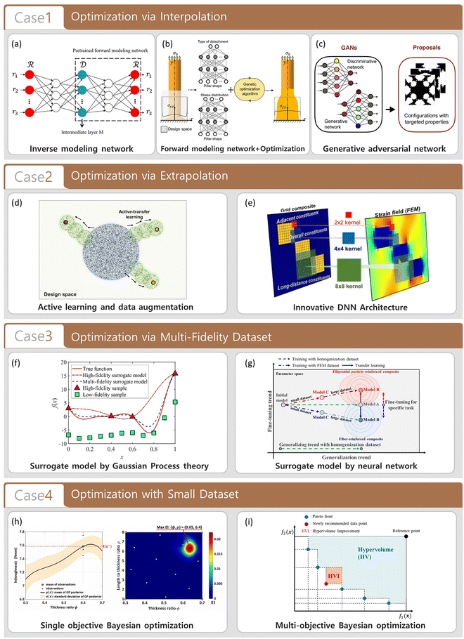 | ||
| Fig. 1 This figure presents the four major types of inverse design problems in the context of ML-based methods in materials design and manufacturing, alongside representative research examples for each case. Case 1 Illustrates scenarios where there is a wealth of data and a relatively constrained design space. The figure showcases (a) Inverse modeling network (Reproduction with permission from ref. 65. Copyright (2018) American Chemistry Society), (b) Forward modeling network coupled with optimization algorithm (Reproduction with permission from ref. 59. Copyright (2020) American Chemistry Society), and (c) Generative adversarial network (From ref. 93, Licensed under CC BY-NC 4.0) as examples of effective interpolation strategies in this context. Case 2 depicts large design space scenarios and the associated challenges of weak generalization performance of ML models. (d) Active learning and data augmentation (From ref. 100, Licensed under CC BY 4.0) and (e) Innovative DNN architecture (Reproduction with permission from ref. 106. Copyright (2022) Elsevier) are featured as solutions to enhance generalization and extrapolation in unseen domains. Case 3 highlights the challenge of reconciling differences between diverse datasets. Research approaches such as the (f) Surrogate model by Gaussian process theory (Reproduction with permission from ref. 111. Copyright (2022) Elsevier) and the (g) Surrogate model by neural network (Reproduction with permission from ref. 128. Copyright (2022) Elsevier) are showcased as potential solutions. Case 4 presents the conundrum of limited dataset and a small design space. (h) Single objective Bayesian optimization (Reproduction with permission from ref. 134. Copyright (2022) Elsevier) and (i) Multi-objective Bayesian optimization (Reproduction with permission from ref. 104. Copyright (2022) Springer Nature) are included as strategies to achieve optimal design under these circumstances. | ||
2. Inverse design using interpolation of AI model (case 1)
ML constructs AI surrogate models that can approximate the output (material performance) as a function of input design variables (structure or process parameters). In particular, deep learning (DL) has enabled a superior prediction compared to conventional ML by using an artificial neural network-based surrogate model that leverages a big data set to learn the complex input–output relationship.29 The DL-based black-box predictor has allowed researchers to have limited domain knowledge or experience to infer the correlation between the input and the output of a given problem. Many existing studies applied DL to solve various inverse design problems by training a model first and then exploring the optimum in the design space using the trained model.59–63In this section, we investigate the case of an inverse design problem in which the optimal design configuration does not deviate significantly from the scope of the initial training set. Here we refer to such a case as an interpolation problem. To effectively tackle the interpolation problem, we provide some representative ML-based strategies that are suitable for the case where the amount and reliability of available data are sufficient to describe the input–output relation over the entire design space. For such case, the initially trained ML model generally have an excellent predictive performance over the entire design space, and thus, the optimum design can be found without having to update the ML model during the optimization. Inverse modeling network, a forward modeling network combined with a conventional optimization scheme, and a recently emerged generative adversarial network (GAN) will be reviewed in this section.
2.1. Inverse modeling network
An inverse modeling network refers to a neural network trained to predict a design variable as an output while the material performance is given as an input. After training the network, a researcher can use the trained model to determine the optimal values for the design variables by simply entering the desired performance as an input. The method is highly efficient in terms of time as the trained neural network can recommend the optimal designs within a very short time. However, when multiple sets of design variables have identical performance, the training of the neural network for inverse design is difficult as conventional DNN models cannot effectively capture the one-to-many mapping.64,65Several subsequent studies tried to improve the inverse model approach to overcome the limitation. Kabir et al. (2008) trained an inverse design neural network that predicts the values of geometrical parameters by putting the electrical parameters as input and then used the trained surrogate model for designing microwave guide filters. At first, the study divided the given training data set into different groups in a way that each group does not contain the samples having the same performance but different designs. Then, they constructed multiple inverse modeling networks for each group of training sets, which were later integrated into one form of a comprehensive prediction model. As a result, the proposed method showed higher prediction accuracy than the conventional DNN models that are trained with all training samples at once (Fig. 2).64
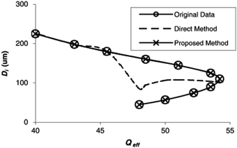 | ||
| Fig. 2 Comparison of the predictions made by the inverse modeling network trained using the direct inverse modeling method and the proposed division method for microwave guide filter design. The figure presents the predicted relationship between the inner mean diameter (Di) of a spiral inductor and the effective quality factor (Qeff). Applying the proposed division method reduces the error significantly, decreasing it from 13.6% to 0.05%. Reproduction with permission from ref. 64. Copyright (2008) IEEE. | ||
However, although the division method could be readily implemented for the inverse design problems that have a small and simple data structure, division of the training data was far more challenging when it came to a complex design space. Hence, as an alternative solution, Liu et al. (2018) proposed a tandem network architecture, whose structure has an inverse modeling network attached in front of a forward modeling network as described in Fig. 3. To model the correlation between design and response (performance), the forward modeling network located at the back of the architecture (right side of the figure) is trained first. After fixing the weights trained in the previous step, the remaining inverse modeling network is trained to reduce the error between the predicted response and the desired response. Finally, the trained tandem network was able to generate a design candidate on the intermediate layer M by putting the desired response as an input. Even if there were multiple design solutions for one identical response in the training dataset, the forward modeling network depicting many-to-one mapping was trained accurately. Furthermore, since the inverse modeling of the second training stage did not aim to predict the real design of the train data, the network could be trained effectively despite the data inconsistency. In this study, the proposed tandem-shaped network was applied for the designing of a nanophotonic structure that has the desired performance.65
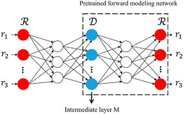 | ||
| Fig. 3 Proposed tandem-shaped neural network for inverse design problem of the nanophotonic structure. The forward modeling network is represented by dashed lines, with the inverse modeling network attached in front. The red nodes represent the response, while the blue nodes represent the design variables. Reproduced with permission from ref. 65. Copyright (2018) American Chemistry Society. | ||
The approach employing the inverse modeling network carries the benefit of rapidly proposing optimal design candidates once the neural network is trained. Consequently, this strategy has found applications across a range of inverse design problems.66–71 However, the dimension of the input variables that correspond to the material performance is usually lower than the dimension of the output variables that correspond to the materials design parameters, thereby limiting the dimension of the recommended optimal values. Such a problem may not be an issue in the case of simple problems in which the dimension of design variables is relatively small, but the strategy may not be applicable to more complex design problems with higher input and output dimensions.
2.2. Forward modeling network + optimization
A forward modeling network, as opposed to an inverse modeling network, is an AI model that predicts the material performance for a given set of design parameters.65 The forward model has no difficulty in training, even if multiple sets of design variables have identical performance values or if the dimension of design variables (input) is much larger than the dimension of performances (output). A well-trained AI model can produce reliable prediction results in a fraction of a second, replacing the time-consuming simulations or experiments that are conducted for the evaluation of objective functions.In a sequential optimization strategy where the optimization process gradually approaches the global optimum by repeatedly augmenting new data to the model, the acquisition of a new dataset may take a considerable amount of time if numerous iterations of data augmentation are taken. This is especially true when we use computer simulations and experiments that cost significant time to predict the material performance for a given design variable set. Therefore, many studies have been conducted to efficiently find the optimum by combining the AI surrogate model while following the workflow of the existing data-driven optimization algorithm. For instance, Kim et al. (2020) combined the forward modeling network with the conventional genetic algorithm to optimize the structures of an axisymmetric adhesive pillar. In this study, a DNN-based surrogate model is trained with its input being 501 design variables that characterize the 2D shape of an adhesive pillar and its output being the interfacial stress distribution at the boundary between the pillar and a substrate. The stress distribution was compressed into 30 valid features through principal component analysis (PCA) for efficient training of the neural network. Also, in order to select adhesive pillars with the desired detachment type, an additional DNN for classification was trained. The trained neural networks were able to predict the output accurately and quickly for 1000 proposed adhesive pillar designs. Based on the predictive power of the networks, the genetic algorithm was performed, and the optimal pillar shapes that can minimize the interfacial stress singularity were found, as shown in Fig. 4.59 There are many other studies that performed optimization by combining the forward modeling network with optimization algorithms in various design problems.72–79
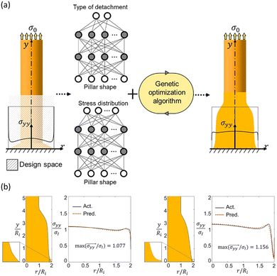 | ||
| Fig. 4 (a) Design space and schematic of inverse design of the shape of the adhesive pillar combining the forward modeling network and the genetic algorithm. (b) Cross-sectional area and distribution of interfacial stress (σyy) normalized by ideal flat stress (σI) distribution for optimized adhesive pillar design with a sharp edge (Left) and a truncated edge (Right). Reproduction with permission from ref. 59. Copyright (2020) American Chemistry Society. | ||
A different approach called generative inverse design network finds the optimal designs having the desired performance by using back-propagation in neural networks. Generally, back-propagation is a process of optimizing the hyperparameters of hidden layers to minimize the loss function, the value of which quantitatively defines the error between the network's predicted result and the ground truth value.80 After the training stage, we can find the optimal design by fixing all neural network parameters except for the input features so that the input values are tuned to minimize a loss function through back-propagation.81,82
For example, Peurifoy et al. (2018) solved the inverse design problem using the back-propagation-based approach to find the optimal thickness combination of nanoparticle causing desired light scattering spectrum.81 First, to construct the AI regression model, the neural network was trained by the data collected from light scattering simulation, which generates the light scattering spectrum for a set of parametrized thickness values of multi-layered nanoparticles. Then, by fixing all weights except for the input features, the optimized particle designs having the desired scattering spectrum were obtained through back-propagation. The study demonstrated that the neural network (NN) outperformed the numerical non-linear optimization method by achieving a significantly closer minimum in some cases (Fig. 5).
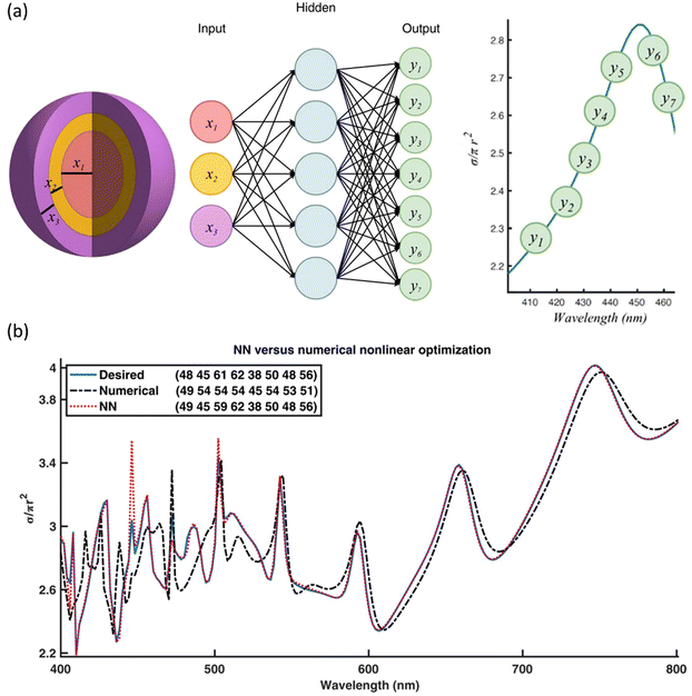 | ||
| Fig. 5 (a) Schematic of the neural network predicting the scattering cross section (σ/πr2) at varying wavelengths from the thickness value of each shell of the nanoparticle. (b) The desired spectrum (Blue), the spectrum from the NN-based design method (Orange dashed), and the spectrum from the non-linear numerical optimization method (Black dashed) for an eight-shell nanoparticle made of alternating shells of TiO2 and silica. The numbers in the legend denote the designed input shell thickness. From ref. 81, Licensed under CC BY-NC 4.0. | ||
2.3. Generative adversarial network (GAN)
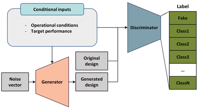
The capability of DL to perform classification tasks further improved the inverse design framework by classifying whether a new design is realistic or not. GAN (Generative Adversarial Network) is a representative neural network architecture that adversarially trains a generator that creates data and a discriminator that judges whether the created data is similar to the original data set or not, in order to generate new but still reasonable data close to real training data.83 The GAN has been adopted for research mainly related to image processing,84–86 and it is now rapidly expanding to various applications, such as the medical industry,87,88 natural language processing,89 and voice recognition.90GAN has also been employed to solve inverse design problems as it can find a new design candidate with excellent predictive performance, a design that is still similar to the designs within the original training set.91–93 Additionally, modified forms of GANs, such as conditional GAN (CGAN)94 and Wasserstein GAN (WGAN),95 further expanded the scope of inverse design by making the training of the model easier and expanding the types of tasks that the DL can perform.96–98
For example, Kim et al. (2020) applied WGAN structure to build a network called ZeoGAN and solved the inverse design problem of porous material to obtain the desired level of methane heat absorption. Engineered to address common challenges in traditional GANs such as unstable training and mode collapse, the WGAN introduces a novel role for the discriminator. Unlike in a traditional GAN, where the discriminator only verifies the authenticity of data, the discriminator in a WGAN (often referred to as a critic to highlight the difference in roles) is programmed to compute the Earth-Mover's distance (EMD) or the Wasserstein distance, which quantifies the minimal effort required to reshape the actual data distribution to match the artificial one. This serves as a robust indicator of their similarity. The WGAN's strategy of using the critic to calculate the EMD leads to improved stability during training and more precise evaluations of data similarity. This significantly boosts the efficiency of the training process, resulting in the generation of high-quality, realistic data. In this research, the generator that can create a structure and energy distribution similar to that of porous material from noise input was trained, and the optimal candidates were obtained by modifying the generator's loss function to obtain the desired methane heat of absorption (Fig. 6). Since the generator can be trained for other target properties, and the identical framework can be applied to other gases, the expandability of the optimization framework proposed in this research is superb.97
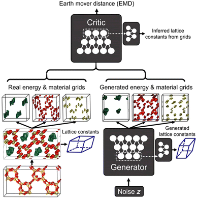 | ||
| Fig. 6 Schematic representation of ZeoGAN architecture employed for inverse design of porous material. The generator and critic components were trained to minimize the EMD between real and generated inputs composed of materials grids (red representing silicon atoms and yellow representing oxygen atoms) and methane potential energy (green). An auxiliary neural network was trained to explicitly predict the lattice constant. From ref. 97, Licensed under CC BY-NC 4.0. | ||
As another example, Yilmaz & German (2020) conducted an Airfoil inverse design study using CGAN. Unlike GAN, CGAN puts a conditional vector during training to limit or to add conditions to the image generated by the generator. In this study, the neural networks were trained to generate only the design of the airfoil shape with the desired stall angle by adding the design range and angle of attack of the aircraft wing as a conditional vector. As a result, various airfoil designs that satisfy the required stall angle condition were successfully obtained (Fig. 7).98
3. Inverse design requiring extrapolation (case 2)
Recently, the development of manufacturing techniques, such as additive manufacturing, enables the production of materials with very complex topologies, expanding the design space of material structures astronomically. In such humongous design spaces, a randomly generated initial training dataset of average size is usually not informative enough to capture the input–output relationship over the entire design space. Therefore, an extrapolation task has to be performed to explore the design space to find the optimal designs having characteristics significantly different from the initial training set. Although the forward modeling network has high accuracy in predicting the performance of the designs similar to the training data set, the network loses its predictive power when it comes to the unseen design domain far beyond the initial data set.44–50 Therefore, for the inverse design problem having a vast design space, the extrapolation issue of the neural network should be handled.The second section introduces AI model-based inverse design methodologies considering a vast design space and extrapolation tasks. The methods can be applied to inverse design problems in which the data has sufficient fidelity, yet the amount is not enough to describe the whole design space. Active learning strategy and novel network architecture will be reviewed in this section to effectively explore the unseen design domain.
3.1. Active learning-based approach
Active learning refers to an ML strategy where the computation model selects the training data by itself and uses it for the training. In addition, active transfer learning is a training method that updates and improves the pre-trained neural network with the dataset selected by the computer itself.99,100 Iterative use of active transfer learning can train the neural network so that the model can more accurately predict the performance of the dataset far from the initial training set. Therefore, the deep learning-based optimization framework based on active transfer learning combined with appropriate new candidate designs provides a clue to the extrapolation challenge in various engineering problems.For example, Kim et al. (2021) proposed a DNN-based forward design framework to explore the unseen design space efficiently. For instance, researchers have undertaken the optimization task of organizing stiff and soft materials to maximize mechanical properties such as stiffness, strength, and toughness, within an 11 × 11 grid composite consisting of 71 stiff and 50 soft blocks. The forward modeling network, trained on an initial training dataset of 100![[thin space (1/6-em)]](https://www.rsc.org/images/entities/char_2009.gif) 000 randomly arranged samples from an enormous possibility space of 1.8 × 1034 configurations, demonstrated limited predictive capability for well-ordered configurations significantly diverging from the initial dataset. The proposed method in this study gradually reinforced the DNN model through active learning by repeatedly training the model with the new candidate designs suggested by greedy sampling and a genetic algorithm. Such a sequential training method allowed the model to propagate toward the optimal designs having excellent mechanical stiffness and strength in the vast design space (Fig. 8). The study shows that a new composite design with optimal stiffness and strength can be found in a very efficient way, the size of the augmented dataset, computed by material descriptor, being only 0.5% of that of the initial dataset. The study also highlighted that the surrogate model must at least have a ‘reasonable’ extrapolation performance, if the model is to be used for the greedy sampling and genetic algorithm. For example, the DNN model used in this study was trained with the data having low material properties (lower 90%) in terms of stiffness and strength, and the model resultantly showed inevitable prediction errors when it was dealing with the designs having top 10% material properties, as the model was carrying out an extrapolation task. However, although the model was not able to accurately predict the values of stiffness and strength for the designs, the model was capable of determining the relative ranking of the designs by their performance. As a result, the surrogate could be combined with the greedy sampling algorithm and genetic algorithm, together forming the active transfer-learning framework. However, the same approach could not be adopted for the optimization of composite for toughness, which corresponds to the total area under the stress–strain curve, as the DNN model failed to show the minimal predictive power to carry out the ranking of the predicted designs. Insufficient predictive power can be improved based on domain knowledge from solid mechanics.100
000 randomly arranged samples from an enormous possibility space of 1.8 × 1034 configurations, demonstrated limited predictive capability for well-ordered configurations significantly diverging from the initial dataset. The proposed method in this study gradually reinforced the DNN model through active learning by repeatedly training the model with the new candidate designs suggested by greedy sampling and a genetic algorithm. Such a sequential training method allowed the model to propagate toward the optimal designs having excellent mechanical stiffness and strength in the vast design space (Fig. 8). The study shows that a new composite design with optimal stiffness and strength can be found in a very efficient way, the size of the augmented dataset, computed by material descriptor, being only 0.5% of that of the initial dataset. The study also highlighted that the surrogate model must at least have a ‘reasonable’ extrapolation performance, if the model is to be used for the greedy sampling and genetic algorithm. For example, the DNN model used in this study was trained with the data having low material properties (lower 90%) in terms of stiffness and strength, and the model resultantly showed inevitable prediction errors when it was dealing with the designs having top 10% material properties, as the model was carrying out an extrapolation task. However, although the model was not able to accurately predict the values of stiffness and strength for the designs, the model was capable of determining the relative ranking of the designs by their performance. As a result, the surrogate could be combined with the greedy sampling algorithm and genetic algorithm, together forming the active transfer-learning framework. However, the same approach could not be adopted for the optimization of composite for toughness, which corresponds to the total area under the stress–strain curve, as the DNN model failed to show the minimal predictive power to carry out the ranking of the predicted designs. Insufficient predictive power can be improved based on domain knowledge from solid mechanics.100
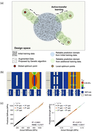 | ||
| Fig. 8 (a) Gradual expansion of reliable prediction domain through data addition using NN prediction-based genetic algorithm (b) optimized grid composite configuration for stiffness (Left) and strength (Right) (c) Increase in the stiffness (Left) and strength (Right) of grid composites on each update of the NN prediction-based genetic algorithm. From ref. 100, Licensed under CC BY 4.0. | ||
The active transfer learning-based framework has been successfully applied to the optimization of composites and structures for other target properties. Demeke et al. (2022) adopted the active transfer learning-based optimization framework for the inverse designing of a thermoelectric power generator to achieve high power and efficiency.101 Lee et al. (2022) found a superb lattice structure with high stiffness and strength by applying the framework to the optimization problem of the density and mechanical properties of the lattice structure constituting the crisscross pattern of beam elements. As above, the adaptive framework has provided a solution to the optimization problem with a myriad of possible shapes.102
On the other hand, optimization using back-propagation combined with active transfer learning also enables an exploration method toward the wider design. Chen and Gu (2020) introduced a generative inverse design networks (GIDNs) framework recommending optimal designs based on back-propagation and active learning. The GIDNs framework proceeds in three stages: predictor training, recommendation of optimum based on back-propagation, and active transfer learning. In the predictor training stage, the AI surrogate model that predicts the output performance of an unknown input design is trained with the initial training samples. Next, the desired values are put into the output layer, the weight of the hidden layer is fixed, and the optimal design candidates are recommended using back-propagation. Finally, the study proceeds with active transfer learning, which evaluates the actual performance of the recommended candidates so that the new data set can be used for the updating of the predictor. By iteratively performing the process above, the predictor is gradually updated to have high predictive power for higher-performance designs that are far from the initial training data (Fig. 9a). This study optimized the geometrical configuration of a grid composite structure, a 2D array of stiff and soft materials ordered in a random manner, to design a higher-toughness composite using the aforementioned inverse materials design method. The size of the initial training dataset was 800![[thin space (1/6-em)]](https://www.rsc.org/images/entities/char_2009.gif) 000, and the designer network recommended 800
000, and the designer network recommended 800![[thin space (1/6-em)]](https://www.rsc.org/images/entities/char_2009.gif) 000 data for active learning in each iteration. The number of data points needed for optimization was significantly smaller compared to the vast number of possible combinations (2128) in the grid composite. Through this study, it was observed that the algorithm based on GIDNs and active learning was capable of identifying high-toughness designs that were not attainable with the initial predictor (Fig. 9b).103
000 data for active learning in each iteration. The number of data points needed for optimization was significantly smaller compared to the vast number of possible combinations (2128) in the grid composite. Through this study, it was observed that the algorithm based on GIDNs and active learning was capable of identifying high-toughness designs that were not attainable with the initial predictor (Fig. 9b).103
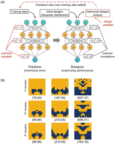 | ||
| Fig. 9 (a) The schematic of Generative Inverse Design Networks (GIDNs). The predictor is a trained DNN that predicts performance outputs based on input design variables, minimizing the error between real and predicted values. The designer produces optimized designs by back-propagation. The optimized designs are utilized for active learning, updating both the predictor and designer for further iterations. (b) Increase of grid composite toughness during each iteration of the GIDNs-based optimization process for three different volume fractions (12.5%, 25%, and 50%). The numbers displayed below the composite configurations represent their corresponding toughness values. From ref. 103, Licensed under CC BY 4.0. | ||
Furthermore, Jung et al. (2022) proposed a process parameter optimization method for the injection molding process using constrained GIDN (CGIDN). The conventional GIDN has a limitation in that the recommended input design from the desired output is unbounded. The CGIDN proposed in the study recommends the process parameter set within a desired range by applying a constraint to the input layer via the sigmoid function. As a result, they were able to find the optimal injection molding process parameter set that simultaneously minimizes deflection after injection and the cycle time required for production.104
3.2. Extrapolation via improved DNN architecture
As an alternative approach, the extrapolation performance of a DL model can also be significantly improved by devising a better architecture of neural networks. Recently, Park et al. (2022, 2023) proposed modified neural network architectures, aiming to discover material structures with superior mechanical properties105 and predict stress and deformation distributions for material designs that are very different from the training set.106Previously, the U-Net architecture, which has shown successful results in image-to-image regression in various engineering and scientific fields, is being utilized to predict the local stress field for an unknown configuration of the grid composite. U-Net was able to successfully predict the stress and strain field corresponding to the composite constituents by compressing the composite shape spatial information and supplementing and expanding the compressed information. Yet, U-Net predicts the material local fields without considering various spatial kernel effects, and it drops a lot of information from an algorithmic point of view. Hence, it was difficult to guarantee the generalizability of the model for a vast design space, indicating that U-Net still has limitations in making the predictions for a grid composite structure that is very different from the training datasets in terms of the relative volume fraction (VF) of the two constituent materials.107
To enhance the generalizability of the prediction model, it is crucial to thoroughly capture the correlation between the arrangement of two constituents for the grid composite and local mechanical deformation. For this purpose, Park et al. (2022) proposed a neural network architecture that combines various kernels of different sizes, rather than using fixed-sized kernels as in the U-Net, to efficiently extract the relationship between composite configuration and strain field at multiple scales. Specifically, the convolutional unit in the encoder section simultaneously utilizes three varying kernel sizes: 2 × 2, 4 × 4, and 8 × 8 (Fig. 10a), allowing effective usage of both local and global information in grid composites. The feature maps from these kernels are subsequently merged through a feature fusion layer (addition) and carefully concatenated using skip connections to mitigate gradient loss. The concatenated feature maps are then squeezed by bottleneck layers and passed through max-pooling layers to reduce the dimension of the feature maps while preserving meaningful information. Fig. 10b illustrates a schematic of a multi-dense block structure describing the aforementioned process. After then, this study applied the transpose convolution operation in the decoder section to recover the dimension of the feature maps reduced in the encoder section.
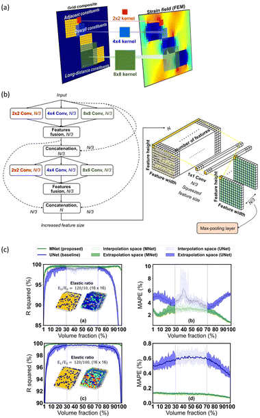 | ||
| Fig. 10 (a) Feature extraction using multiple kernels having varying sizes. (b) The schematic of multi-dense block structure. (c) Comparison of generalizability of M-Net and U-Net. M-net shows better predictive power on the extrapolation test. Reproduction with permission from ref. 106. Copyright (2022) Elsevier. | ||
The proposed M-Net architecture successfully predicted the strain field of the grid composite structure that has a VF that is significantly different from the designs in the training set (Fig. 10c). In addition, this modified model showed the equivalent predictive performance even with a data set 1/3 times smaller than that used for the existing model. This research clearly showed that one can redesign the DNN architecture to efficiently tackle the purpose of the optimization problem. Here, the modified network exhibited an excellent extrapolation performance near the optimal design, even without the sequential active learning process introduced in the previous section.
Furthermore, Park et al. (2023) proposed a double generative network (DGNet) to explore the design space over extrapolation areas having higher effective stiffness compared to the initial training dataset. This model aims to predict stress and strain fields from the composite material configuration and derive effective stiffness from the predicted stress field. In order to sequentially utilize the shape and grid-averaged fields as input features for predicting composite stress fields, Park suggested the deep learning framework that c onsists of two generators based on the M-Net architecture. The first generator predicts grid-averaged fields, which are then put into the second generator, producing high-resolution stress fields. To ensure generalized predictive performance in extrapolation regimes, a CGAN was utilized to train the deep learning framework adversarially (Fig. 11). The proposed deep learning framework accurately predicted structures with superior stiffness compared to the initial training dataset, while the conventional U-Net showed a significant degradation in predictive performance in the extrapolation areas.105 We foresee more research works toward new DNN architecture design in the material/structure optimization field to enable faster and more efficient search for the optimal materials design outside the initial training set.
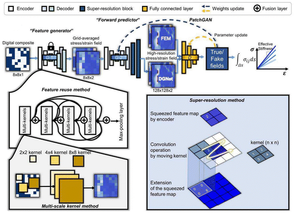 | ||
| Fig. 11 The architecture of DGNet. The DGNet is composed of two generators the G-1 and the G-2. The G-1 generates a grid-averaged image from the shape of the digital composite, and the G-2 generates a high-resolution stress/strain field image. The DGNet is trained adversarially, and effective stiffness is estimated from the generated high-resolution image. Reproduction with permission from ref. 105. Copyright (2023) Elsevier. | ||
4. Inverse design with multi-fidelity datasets (case 3)
This section addresses data-driven design methods applicable to multi-fidelity datasets. Multi-fidelity datasets mean that there exist datasets with different levels of fidelity information. These multi-fidelity approaches allow for more efficient problem-solving by managing the trade-off between accuracy and computational efficiency in modeling. Before the multi-fidelity surrogate model was developed, problems were commonly solved using only highly accurate models, which typically demand significant computational resources. The multi-fidelity surrogate technique can mitigate this difficulty by integrating a limited amount of accurate high-fidelity data with a large amount of less accurate low-fidelity data. It thus utilizes a large amount of low-fidelity data to identify overall trends and a relatively small amount of high-fidelity data to calibrate the models, facilitating a faster and more efficient generation of an accurate surrogate model compared to using high-fidelity data alone. This paper categorizes methods for constructing multi-fidelity surrogates into two approaches: multi-fidelity surrogates based on (1) Gaussian processes and (2) neural networks. In addition, optimization methodologies and engineering applications using the multi-fidelity surrogate model are investigated.4.1. Multi-fidelity surrogates using Gaussian process
In this section, the Gaussian process-based multi-fidelity surrogate model is explained. This model has the advantage of providing uncertainty estimation, which delivers confidence intervals for predictions. However, it comes with the disadvantage of extensive modeling time and difficulty in accurate hyperparameter estimation when dealing with large-scale datasets, thus limiting its effectiveness. As a result, Gaussian process-based multi-fidelity surrogates are most effective on small to medium-sized datasets.Two notable approaches exist for Gaussian process-based multi-fidelity surrogate modeling. One approach involves constructing an extended correlation matrix that considers the relationship between low- and high-fidelity data.108 The other approach entails creating a low-fidelity surrogate model first and then using high-fidelity data to correct this low-fidelity surrogate model.109 While both methods exhibit superior performance compared to traditional single-fidelity surrogate models, the relative superiority between the two methods has not been thoroughly validated. However, in cases where low-fidelity data is abundant and inexpensive, and where there is a possibility of generating additional high-fidelity data, the latter approach is in general known to be more efficient from the perspective of surrogate modeling.
Fig. 12 illustrates a single-fidelity model created using only high-fidelity data, and a multi-fidelity model built by incorporating low-fidelity data. The multi-fidelity surrogate model outperforms the high-fidelity surrogate model in terms of accuracy, as shown in Fig. 12. This superior performance can be attributed to the low-fidelity data effectively capturing the overall trend of the high-fidelity system.
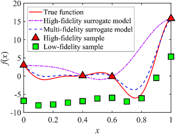 | ||
| Fig. 12 Concept illustration of multi-fidelity surrogate modeling. Reproduction with permission from ref. 111. Copyright (2022) Elsevier. | ||
Numerous studies have demonstrated that multi-fidelity surrogates are applied by categorizing high- and low-fidelity models based on various criteria. For instance, Guo et al. (2021) and Lee et al. (2022) distinguished between high-fidelity models (fine mesh) and low-fidelity models (coarse mesh) by implementing different mesh sizes for variable stiffness composites and railcar structures, respectively.110,111 Yong et al. (2019) distinguished high-fidelity models (3D elements) and low-fidelity models (2D elements) by using different mesh types for gas turbine engines.112 Moreover, Liu et al. (2020) developed a low-fidelity model of mesostructure using homogenized effective dynamic properties.113 In light of these examples, high- and low-fidelity models can be differentiated based on experiments/simulations, simulations/analytical functions, or non-linear solvers/linear solvers, among others, depending on the situation. Moreover, instead of considering only two fidelities (i.e., bi-fidelity), the multi-fidelity approach can be extended if experiments or analytical functions are available. In such cases, fidelities can be divided into levels such as experiment, high-fidelity simulation model, low-fidelity simulation model, and analytical function, and so on.
Some studies have attempted to determine whether or not to utilize multi-fidelity surrogate models. Various approaches based on maximum likelihood estimation,114 normalized cross-validation error,114 and Pearson correlation coefficient115,116 metrics have been proposed. The performances of these methods do exhibit some limitations, as reported in ref. 114–116. However, to sum up, the literature review, the consensus among most studies is that higher values of the Pearson correlation coefficient generally recommend the use of multi-fidelity models over single-fidelity models.
As an application example, Lee et al. (2022) applied the Gaussian process-based multi-fidelity surrogate framework to a real-world large-scale system. They constructed high- and low-fidelity models of a railcar structure with a difference in mesh density, as showin in Fig. 13. The computational cost ratio between the high- and low-fidelity model was 70, and the relative error in accuracy between the two models was approximately 70%. Furthermore, since the value of the Pearson correlation coefficient between the low-fidelity and high-fidelity data exceeded 0.9, it is recommended to create a multi-fidelity surrogate model. In this study, a single-fidelity model was created using the Kriging method with 15 high-fidelity samples. In addition, the hierarchical Kriging model, which is one of multi-fidelity surrogate modeling methods, was constructed utilizing the same 15 high-fidelity samples and additional 100 low-fidelity samples. As a result of comparing the performance of the two models, the accuracy increased by about three times while the computational costs remained almost the same. Moreover, both accuracy and efficiency improved compared to a Kriging model that used 20 high-fidelity samples. Through this application, it was demonstrated that the performance of the multi-fidelity framework was superior to that of the single-fidelity framework in terms of both accuracy and efficiency.111
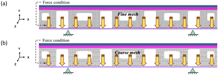 | ||
| Fig. 13 Finite element model of railcar with 5 design variables: (a) side view of high-fidelity model and (b) side view of low-fidelity model. Reproduction with permission from ref. 111. Copyright (2022) Elsevier. | ||
When low-fidelity data is not significantly cheaper than high-fidelity data, an adaptive sequential sampling approach should be employed to efficiently find optimal solutions.117–119 In such cases, appropriate utilization of low- and high-fidelity data is crucial. Huang et al. (2006) suggested the Co-Kriging-based sequential sampling method, introducing a measure utilizing the cross-correlation coefficient and cost ratio between low- and high-fidelity models.117 Subsequently, Zhang et al. (2018) proposed the variable-fidelity expected improvement method, which is a hierarchical Kriging-based sequential sampling method.118 This method provides information on the location and fidelity level of the next sample point using scaling factor and uncertainty information of low-fidelity and high-fidelity models. Furthermore, when parallel computing is possible, strategies for efficient sequential sampling in the allocated batch size have been investigated.120 Through these sequential sampling strategies, the optimization process can be efficiently conducted without wasting not only high-fidelity data but also low-fidelity data. Therefore, the effectiveness of these approaches compares favorably to simply adding either high-fidelity or low-fidelity data.
4.2. Multi-fidelity surrogates using neural network
In this section, neural network-based multi-fidelity surrogate models are illustrated. These models offer the advantage of being relatively fast and accurate for large-scale datasets compared to the Gaussian process-based models. However, it comes with potential drawbacks, such as a higher risk of overfitting when data is insufficient. In addition, neural network-based models generally face more difficulty in uncertainty estimation and require careful hyperparameter setting (e.g., the number of hidden layers and activation function) compared to the Gaussian process-based models.In the era of big data, many researchers are actively employing neural network-based multi-fidelity surrogate models. In such models, a loss function consisting of the difference between predicted and true values (e.g., mean squared error) is typically minimized to estimate the hyperparameters (e.g., weights and biases). If multi-fidelity datasets are available, an additional loss term is further added to construct the original loss function specifically for the neural network-based multi-fidelity surrogate model. This approach has been successfully applied to a variety of engineering problems.55,121–123 Moreover, if low-fidelity data is used to incorporate information from analytical functions (e.g., partial differentiation equations), this concept aligns with the idea of physics-informed neural networks.124,125
In addition, the concept of transfer learning can also be applied to handle multi-fidelity datasets. Transfer learning is a strategy to construct a neural network to learn input–output correlations of the desired dataset (typically, a small dataset with high fidelity) by using the dataset to perform fine-tuning of a pre-trained network, which is initially trained with a preliminary dataset (typically, a big dataset with low fidelity). The fine-tuning process of the transfer learning refers to either selecting only a few hidden layers from the pre-trained neural network for the training, or slightly modifying the overall weights in a reduced learning rate and epoch. Hence, if a pre-trained model exists for a similar task (that pertains to the preliminary dataset), it is easier to develop a surrogate model of our interest, as the fine-tuning of the pre-trained model generally requires a dataset of relatively small size. Owing to this advantage, the transfer learning drew big attention particularly in the research fields that have multiple sources of data, one domain where data can be easily collected and another domain where data acquisition is difficult.126
For example, Xu et al. (2021) applied the transfer learning technique in building an AI surrogate model that predicts the material properties of grid composites from the microstructure of composites. At first, the study developed a pre-trained CNN model that predicts the statistical parameter datasets (500), called as the analytical solution of geometry and distribution features (ASGDF), for a given grid configuration, which pertains to a problem whose input–output data can be computed relatively easily. After that, the pre-trained CNN was fine-tuned by the smaller number of FEM datasets (208) so that the final model could predict the effective elastic modulus of the composite. By using transfer learning, it was possible to reduce the amount of FEM data for CNN training by half (Fig. 14).127
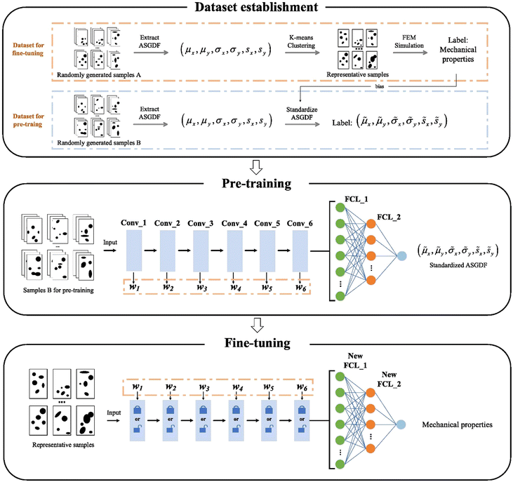 | ||
| Fig. 14 Transfer learning workflow for micro structure–property prediction using CNN. CNN is pre-trained by ASDGF label, which is easier to compute, and CNN is fine-tuned by real mechanical properties. Reproduction with permission from ref. 127. Copyright (2021) Elsevier. | ||
As another example, Jung et al. (2022) used the transfer learning technique to predict the non-linear mechanical responses of fiber-reinforced composites. The mean field homogenization technique can quickly compute the non-linear mechanical response beyond yield for the composites containing ellipsoidal reinforcement based on a few theoretical assumptions. However, if the shape of the reinforcement is not ellipsoidal or the volume fraction of the reinforcement material is higher than 20%, the prediction accuracy drops significantly. In contrast, although it demands higher computational cost and time, the finite element method (FEM) based calculations with fine mesh provide data of higher accuracy compared to that computed with the homogenization theory. This study pre-trained the DNN using the 49![[thin space (1/6-em)]](https://www.rsc.org/images/entities/char_2009.gif) 000 homogenization-based data and then fine-tuned the DNN with the 1400 high-accuracy FEM dataset. As a result, the constructed DNN could accurately predict the elastoplastic response of given composite geometries. The transfer-learned AI model showed higher prediction accuracy than a DNN trained only using FEM data. In the Fig. 15a, the model A refers to homogenization-based data pre-trained model, and the model B is fine-tuned with FEM data from model A. Model C is trained with FEM data only. By fine-tuning to specific target tasks (here, target inclusion geometry), model B can show better prediction performance compared to model C which suffers from overfitting due to insufficient dataset size. Fig. 15b shows model B and C prediction compared to ground truth FEM result for top four maximum relative error cases with ellipsoidal particle reinforced inclusion. Model B shows refined prediction performance compared to model C.128
000 homogenization-based data and then fine-tuned the DNN with the 1400 high-accuracy FEM dataset. As a result, the constructed DNN could accurately predict the elastoplastic response of given composite geometries. The transfer-learned AI model showed higher prediction accuracy than a DNN trained only using FEM data. In the Fig. 15a, the model A refers to homogenization-based data pre-trained model, and the model B is fine-tuned with FEM data from model A. Model C is trained with FEM data only. By fine-tuning to specific target tasks (here, target inclusion geometry), model B can show better prediction performance compared to model C which suffers from overfitting due to insufficient dataset size. Fig. 15b shows model B and C prediction compared to ground truth FEM result for top four maximum relative error cases with ellipsoidal particle reinforced inclusion. Model B shows refined prediction performance compared to model C.128
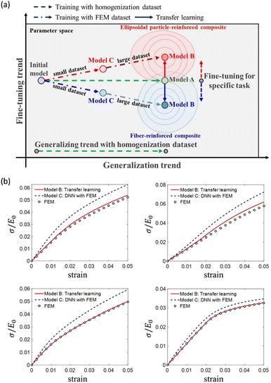 | ||
| Fig. 15 (a) The schematic of the training process of the transfer-learned DNN model for predicting the elastoplastic behavior of fiber-reinforced composites. Model A is trained using a homogenization dataset to capture the overall trend, while Model B is fine-tuned using FEM data to improve the accuracy of exact values. Model C is trained with small FEM dataset which were not sufficient to capture all details and suffer from overfitting. (b) Comparison of Prediction on ground truth FEM data for top four maximum relative error cases for ellipsoidal particle-reinforced composite. Reproduction with permission from ref. 128. Copyright (2022) Elsevier. | ||
In addition, multi-fidelity surrogate models can be combined with an appropriate optimization algorithm to solve the inverse design problem. For instance, Dong et al. (2021) combined a DNN-based surrogate model constructed by transfer learning with conventional data-driven optimization algorithms such as genetic algorithms and Bayesian optimization to inverse-design an optical material (composite metal oxides) having desired light absorption spectrum. To be specific, the purpose of the study is to find a mole ratio of a listed material composition that results in the desired absorption spectrum. The challenge lies in the training of an AI model as a relatively small number of data was available for the materials in the list. To overcome this hurdle, the researchers pre-trained the initial model with a large pool of available datasets, although their material compositions are different from the materials of their interest. After that, they fine-tuned the pre-trained model with a small number of data having the material compositions of their interest. As a result, they were able to construct a surrogate model that can predict the absorption spectrum based on the mole ratio of its material composition. Then, the genetic algorithm and Bayesian optimization were carried out with the transfer-learned surrogate model to discover the optimal design.129
5. Inverse design with accurate and small dataset (case 4)
In this section, we introduce data-driven inverse design methodologies applicable under the presence of a small dataset, obtained through time-consuming experiments or heavy simulations. Under a scarcity of training data, it is difficult to build a DL-based surrogate model, as they generally require a massive amount of training data for the modeling of a complex input–output relationship. The DL-based algorithms introduced in the previous sections generally had two process components; the construction of an AI-based surrogate model followed by the actual optimization process based on appropriate optimization algorithms. In this section, we review a data-driven method that simultaneously explores the design space and searches for the optimal design.5.1. Gaussian process regression combined with Bayesian optimization
Bayesian optimization (BO) is a widely used data-driven optimization method that has the advantage of finding the optimum when only a small amount of data is available, due to the cost of data acquisition being too expensive, and the size of the design space being relatively small. Unlike gradient-based optimization, BO repeatedly recommends a new candidate design based on the ‘acquisition function’, which simultaneously considers the characteristic of exploitation (i.e., searches the region close to the optimum) and the exploration (i.e., searches for the region with large uncertainty in the regression model). Therefore, BO requires a regression model that can quantitatively estimate the expected value and the confidence interval of the expectation simultaneously.130Gaussian process regression (GPR) is a representative regression methodology that can estimate the predicted value and its reliability at the same time.131 GPR assumes that the data points follow a multivariate Gaussian distribution, and defines a covariance function between the data points to calculate the mean which corresponds to the prediction value at an input data point, and the standard deviation which indicates the reliability of the Prediction. The BO algorithm then computes the ‘acquisition function’ of various design candidates based on the mean and the variance estimated by GPR, and the design that has the highest acquisition function value is recommended as the design to be evaluated next. The expected improvement function, one of the most well-known acquisition functions, is calculated as a weighted summation of the exploitation part, which is related to finding a value close to the optimum, and the exploration part, which is related to the uncertainty of the model. The expected improvement function with an appropriate balance between exploration and exploitation should be used in order to effectively approach to the global optimum.132,133
Recently, Park et al. (2022) adopted BO to optimize the toughness of staggered platelet composite structure, which is one of the representative biomimetic composite structures mimicking a nacre. This composite material has a structure in which a stiff material is placed in a brick form on a soft polymer matrix. Because the prediction accuracy of toughness from either analytical models or computer simulations is not satisfactory, authors collected the toughness data by using a 3D printer to build an actual composite and conduct uniaxial tensile tests. With this accurate, yet expensive-to-evaluate, data collection method, they designed the maximum-toughness structure via Bayesian optimization with a relatively small number of experiments. The initial training phase utilized 14 data points, and for the optimization process, only 5 additional data points were required. The results from the study are visualized in Fig. 16.134
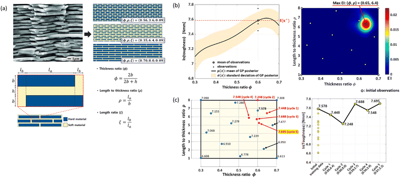 | ||
| Fig. 16 (a) Design variable setting for the optimization of the staggered platelet composite structure. The length ratio (ξ) of this problem is fixed at 0.09. (b) The GPR model for the varying φ while keeping ρ fixed at 6.7. Solid line denotes regression mean, and the shaded area indicates the standard deviation of the regression (Left). Additionally, the heatmap of expected improvement is presented (Right). (c) 14 initial experimental data and 5 data added by BO in each iteration (Left), and the performance values of the data points are depicted (Right). Reproduction with permission from ref. 134. Copyright (2022) Elsevier. | ||
BO can be also extended to solve problems involving multiple objective functions. Multi-objective Bayesian optimization (MBO) aims to find Pareto optimal solutions for multiple objective functions in a trade-off relationship (such as toughness and strength for structural materials, production speed and defective rate for a manufacturing process).135,136 Recently, several studies in materials design and manufacturing adopted MBO to solve inverse design problems with multiple objectives.104,137,138 For example, Jung et al. (2022) applied MBO to optimize the injection molding process parameters and were able to determine the Pareto-optimal process conditions that minimize both the cycle time to produce a single product and the deflection that occurs after production. An initial set of 10 data samples was generated for training GPR-based surrogate model; subsequently, an optimization process was carried out with 250 additional iterations, incorporating the collection of new data points (Fig. 17).104
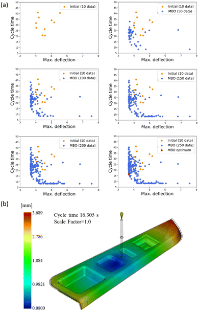 | ||
| Fig. 17 (a) Plot of the results of MBO for every 50 iterations. As the number of iterations increases, the Pareto line becomes more distinct. Design selection can be made from the data points on the plotted Pareto line that meet the specified condition (b) the deflection distribution for the optimized process parameter set comprised of cycle time and maximum deflection. Reproduction with permission from ref. 104. Copyright (2022) Springer Nature. | ||
6. Conclusions
The advancement of ML enables fast and accurate classification and regression for the dataset in the field of materials design and manufacturing. Furthermore, conventional inverse design approaches that rely heavily on people's knowledge and experience can be revolutionized by making the best use of the accumulated dataset through data-driven design methods. A variety of fast and efficient AI model-based algorithms have been proposed over the last few decades and facilitated complex material optimizations even without domain knowledge. However, each of the proposed ML-based methods has its own unique strengths and weaknesses, leaving us with a fundamental question of ‘which ML algorithm to choose’.This review categorizes several ML-based optimization methodologies according to their characteristics of trainable data and the size of the design space. First, in a case where sufficiently large training data is available to capture the input–output trend over the entire design space, inverse modeling networks, conventional optimization methods combined with forward modeling networks, and GAN are suggested as suitable methods. Second, when the initial training set and the optimum are far apart in the vast design space, methodologies resolving the extrapolation challenge are introduced; gradual update of a ML model via the active transfer learning method, and devising an improved neural network architecture. Third, under the presence of two datasets with different fidelities, the domain transfer of an AI model using transfer learning was introduced. Finally, under the scarcity of data due to the objective function being too expensive to evaluate, we suggest a Bayesian optimization framework that makes efficient use of the data to determine the global optimum.
Despite the advent of numerous innovative AI model-based inverse design methods, substantial challenges persist in effectively implementing AI models in manufacturing and materials design sectors. Foremost, procuring initial training data for building the AI surrogate model can be time-consuming, especially for problems with vast design spaces, which demand several hundreds to thousands of initial training data points. Moreover, the issue of extrapolation during the design phase frequently necessitates consideration, even after data acquisition. It is clear that future research must focus on devising methodologies that can efficiently leverage minimal data for inverse design in high-dimensional design spaces. For instance, the physics-informed neural network (PINN) based methodology has been extensively investigated recently to address data paucity and the extrapolation challenge inherent in solving design problems.124,139 Such data-efficient deep learning surrogate models could be integrated with suitable optimization algorithms for inverse design. Furthermore, the quality of data currently accessible in the manufacturing industry remains suboptimal; a large portion of experimental data obtained from the field is either unlabeled or noisy. As a result, research on optimizing parameters in manufacturing processes using ML-based approaches has been less prevalent compared to studies focusing on material composition or structural design. This review primarily discusses inverse design methodologies grounded in supervised learning using labeled data. However, exploration into semi-supervised training-based methodologies, capable of utilizing unlabeled data to create surrogate models, is a promising avenue for further research in data-driven inverse design methods.140,141 Lastly, it's important to note that even in the most straightforward scenario of interpolation, significant errors can often manifest in ML models. Hence, it is crucial not to overly rely on ML and blindly trust its outcomes without checking the quantity and quality of the dataset and the prediction accuracy of the ML model.
In conclusion, ML-based inverse design frameworks have become an innovative route for solving complex inverse design problems that were not handled before. However, it is crucial to choose the right algorithms according to the characteristics of the dataset and design space, and this review provides a concise guideline in the field of materials design and manufacturing. Also, in the future, a design methodology that can exploit small, unlabeled, and noisy data sets should be further investigated to extend the impact of data-driven design methods in more practical engineering applications. At the same time, in addition to the development of algorithms, efforts to establish a database composed of standardized, high-quality datasets should be paralleled.
Author contributions
Junhyeong Lee: conceptualization, writing – original draft, writing – review & editing. Donggeun Park: writing – original draft. Mingyu Lee: writing – original draft. Hugon Lee: writing – review & editing. Kundo Park: writing – review & editing. Ikjin Lee: supervision, writing – review & editing. Seunghwa Ryu: conceptualization, funding acquisition, supervision, writing – review & editing.Conflicts of interest
The authors declare no conflict of interest.Acknowledgements
This work is financially supported by the National Research Foundation of Korea (NRF) (2022R1A2B5B02002365 and RS-2023-00222166).Notes and references
- T. M. Mitchell and T. M. Mitchell, Machine learning, McGraw-hill, New York, 1997 Search PubMed.
- A. A. A. Boulogeorgos, S. E. Trevlakis, S. A. Tegos, V. K. Papanikolaou and G. K. Karagiannidis, IEEE Trans. Mol. Biol. Multi-Scale Commun., 2020, 7, 10–39 Search PubMed.
- S. L. Brunton, J. Nathan Kutz, K. Manohar, A. Y. Aravkin, K. Morgansen, J. Klemisch, N. Goebel, J. Buttrick, J. Poskin and A. W. Blom-Schieber, AIAA J., 2021, 59, 2820–2847 Search PubMed.
- S. L. Brunton, B. R. Noack and P. Koumoutsakos, Annu. Rev. Fluid Mech., 2020, 52, 477–508 CrossRef.
- M. R. Dobbelaere, P. P. Plehiers, R. Van de Vijver, C. V. Stevens and K. M. Van Geem, Engineering, 2021, 7, 1201–1211 CrossRef CAS.
- A. L. Ferguson, J. Phys.: Condens. Matter, 2017, 30, 043002 CrossRef PubMed.
- K. Guo, Z. Yang, C.-H. Yu and M. J. Buehler, Mater. Horiz., 2021, 8, 1153–1172 RSC.
- A. E. Hassanien, A. Darwish and H. El-Askary, Machine Learning and Data Mining in Aerospace Technology, Springer, 2020 Search PubMed.
- M.-P. Hosseini, A. Hosseini and K. Ahi, IEEE Rev. Biomed. Eng., 2020, 14, 204–218 Search PubMed.
- Z. Jin, Z. Zhang, K. Demir and G. X. Gu, Matter, 2020, 3, 1541–1556 CrossRef.
- F.-L. Luo, Machine learning for future wireless communications, John Wiley & Sons, Inc, Hoboken, NJ, 2020 Search PubMed.
- S. J. Nawaz, S. K. Sharma, S. Wyne, M. N. Patwary and M. Asaduzzaman, IEEE Access, 2019, 7, 46317–46350 Search PubMed.
- K. K. Yang, Z. Wu and F. H. Arnold, Nat. Methods, 2019, 16, 687–694 CrossRef CAS PubMed.
- S. Zhong, K. Zhang, M. Bagheri, J. G. Burken, A. Gu, B. Li, X. Ma, B. L. Marrone, Z. J. Ren and J. Schrier, Environ. Sci. Technol., 2021, 55, 12741–12754 CAS.
- J. Jumper, R. Evans, A. Pritzel, T. Green, M. Figurnov, O. Ronneberger, K. Tunyasuvunakool, R. Bates, A. Žídek and A. Potapenko, Nature, 2021, 596, 583–589 Search PubMed.
- D. Silver, J. Schrittwieser, K. Simonyan, I. Antonoglou, A. Huang, A. Guez, T. Hubert, L. Baker, M. Lai and A. Bolton, Nature, 2017, 550, 354–359 CrossRef CAS PubMed.
- P. Linardatos, V. Papastefanopoulos and S. Kotsiantis, Entropy, 2020, 23, 18 CrossRef PubMed.
- A. Adadi and M. Berrada, IEEE Access, 2018, 6, 52138–52160 Search PubMed.
- P. Ren, Y. Xiao, X. Chang, P.-Y. Huang, Z. Li, B. B. Gupta, X. Chen and X. Wang, ACM Comput. Surv., 2021, 54, 1–40 Search PubMed.
- C. Tan, F. Sun, T. Kong, W. Zhang, C. Yang and C. Liu, arXiV, 2018, preprint, arXiv:1808.01974 DOI:10.48550/arXiv.1808.01974.
- J. E. Van Engelen and H. H. Hoos, Mach. Learn., 2020, 109, 373–440 CrossRef.
- S. Omar, A. Ngadi and H. H. Jebur, Int. J. Comput. Appl., 2013, 79, 33–41 Search PubMed.
- L. Scime and J. Beuth, Addit. Manuf., 2018, 19, 114–126 Search PubMed.
- C. A. Escobar and R. Morales-Menendez, Adv. Mech. Eng., 2018, 10, 1687814018755519 Search PubMed.
- R. S. Peres, J. Barata, P. Leitao and G. Garcia, IEEE Access, 2019, 7, 79908–79916 Search PubMed.
- A. Tellaeche and R. Arana, 2013 IEEE 18th Conference on Emerging Technologies & Factory Automation (ETFA), Cagliari, Italy, September 10–13, 2013, ed. C. Seatzu, IEEE, Inc, Piscataway, NJ, 2013, pp. 1–4 Search PubMed.
- S. Tiryaki and A. Aydın, Constr. Build. Mater., 2014, 62, 102–108 CrossRef.
- F. Khademi, M. Akbari, S. M. Jamal and M. Nikoo, Front. Struct. Civ. Eng., 2017, 11, 90–99 CrossRef.
- C. Yang, Y. Kim, S. Ryu and G. X. Gu, MRS Commun., 2019, 9, 609–617 CrossRef CAS.
- Z. Nie, H. Jiang and L. B. Kara, J. Comput. Inf. Sci. Eng., 2020, 20, 011002 CrossRef.
- J. Reiner, R. Vaziri and N. Zobeiry, Compos. Struct., 2021, 273, 114290 CrossRef CAS.
- G. Pilania, C. Wang, X. Jiang, S. Rajasekaran and R. Ramprasad, Sci. Rep., 2013, 3, 1–6 Search PubMed.
- B. Sanchez-Lengeling and A. Aspuru-Guzik, Science, 2018, 361, 360–365 CrossRef CAS PubMed.
- H. Sun, H. V. Burton and H. Huang, J. Build. Eng., 2021, 33, 101816 CrossRef.
- Q. Zhou, S. Lu, Y. Wu and J. Wang, J. Phys. Chem. Lett., 2020, 11, 3920–3927 CrossRef CAS PubMed.
- D. Weichert, P. Link, A. Stoll, S. Rüping, S. Ihlenfeldt and S. Wrobel, Int. J. Adv. Manuf. Technol., 2019, 104, 1889–1902 CrossRef.
- S. Wu, H. Yamada, Y. Hayashi, M. Zamengo and R. Yoshida, arXiv, 2010, preprint, arXiv:07683, 2020.
- A. Bakushinsky and A. Goncharsky, Ill-posed problems: theory and applications, Springer Science & Business Media, 2012 Search PubMed.
- H. Jeong, S. Signetti, T.-S. Han and S. Ryu, Comput. Mater. Sci., 2018, 155, 483–492 CrossRef.
- C. Yang, Y. Kim, S. Ryu and G. X. Gu, Mater. Des., 2020, 189, 108509 CrossRef.
- W. Wang, H. Wang, J. Zhou, H. Fan and X. Liu, Mater. Des., 2021, 212, 110181 CrossRef CAS.
- M. Pathan, S. Ponnusami, J. Pathan, R. Pitisongsawat, B. Erice, N. Petrinic and V. Tagarielli, Sci. Rep., 2019, 9, 1–10 CrossRef CAS PubMed.
- G. X. Gu, C.-T. Chen and M. J. Buehler, Extreme Mech. Lett., 2018, 18, 19–28 CrossRef.
- G. Marcus, arXiv, 2018, preprint, arXiv:1801.00631.
- G. Martius and C. H. Lampert, arXiv, 2016, preprint, arXiv:1610.02995.
- E. Barnard and L. Wessels, IEEE Control Syst. Mag., 1992, 12, 50–53 Search PubMed.
- J. Mitchell, P. Minervini, P. Stenetorp and S. Riedel, arXiv, 2018, preprint, arXiv:1805.06648.
- S. Greydanus, M. Dzamba and J. Yosinski, Adv. Neural Inf. Process. Syst., 2019, 32 Search PubMed.
- Z. Long, Y. Lu and B. Dong, J. Comput. Phys., 2019, 399, 108925 CrossRef.
- A. Kloss, S. Schaal and J. Bohg, Int. J. Robot. Res., 2020, 0278364920954896 Search PubMed.
- J. Schmidhuber, Neural Netw., 2015, 61, 85–117 CrossRef PubMed.
- S. E. Whang, Y. Roh, H. Song and J.-G. Lee, arXiv, 2021, preprint, arXiv:2112.06409.
- A. M. Mroz, V. Posligua, A. Tarzia, E. H. Wolpert and K. E. Jelfs, J. Am. Chem. Soc., 2022, 144, 18730–18743 CrossRef CAS PubMed.
- D. Bishara, Y. Xie, W. K. Liu and S. Li, Arch. Comput. Methods Eng., 2023, 30, 191–222 CrossRef.
- P. Ramu, P. Thananjayan, E. Acar, G. Bayrak, J. W. Park and I. Lee, Struct. Multidiscip. Optim., 2022, 65, 266 CrossRef.
- J. Noh, G. H. Gu, S. Kim and Y. Jung, Chem. Sci., 2020, 11, 4871–4881 RSC.
- Y. Wang, C. Soutis, D. Ando, Y. Sutou and F. Narita, Eur. J. Mater., 2022, 2, 117–170 CrossRef.
- X. Liu, S. Tian, F. Tao and W. Yu, Composites, Part B, 2021, 224, 109152 CrossRef.
- Y. Kim, C. Yang, Y. Kim, G. X. Gu and S. Ryu, ACS Appl. Mater. Interfaces, 2020, 12, 24458–24465 CrossRef CAS PubMed.
- C.-H. Yu, W. Chen, Y.-H. Chiang, K. Guo, Z. Martin Moldes, D. L. Kaplan and M. J. Buehler, ACS Biomater. Sci. Eng., 2022, 8, 1156–1165 CrossRef CAS PubMed.
- B. A. Young, A. Hall, L. Pilon, P. Gupta and G. Sant, Cem. Concr. Res., 2019, 115, 379–388 CrossRef CAS.
- Z. Zhang, Z. Zhang, F. Di Caprio and G. X. Gu, Compos. Struct., 2022, 285, 115233 CrossRef.
- P. Z. Hanakata, E. D. Cubuk, D. K. Campbell and H. S. Park, Phys. Rev. Lett., 2018, 121, 255304 CrossRef CAS PubMed.
- H. Kabir, Y. Wang, M. Yu and Q.-J. Zhang, IEEE Trans. Microwave Theory Tech., 2008, 56, 867–879 Search PubMed.
- D. Liu, Y. Tan, E. Khoram and Z. Yu, ACS Photonics, 2018, 5, 1365–1369 CrossRef CAS.
- J. Jin, C. Zhang, F. Feng, W. Na, J. Ma and Q.-J. Zhang, IEEE Trans. Microwave Theory Tech., 2019, 67, 4140–4155 Search PubMed.
- C. Zhang, J. Jin, W. Na, Q.-J. Zhang and M. Yu, IEEE Trans. Microwave Theory Tech., 2018, 66, 3781–3797 Search PubMed.
- N. A. Alderete, N. Pathak and H. D. Espinosa, npj Comput. Mater., 2022, 8, 191 CrossRef.
- S. Kumar, S. Tan, L. Zheng and D. M. Kochmann, npj Comput. Mater., 2020, 6, 73 CrossRef.
- L. Gao, X. Li, D. Liu, L. Wang and Z. Yu, Adv. Mater., 2019, 31, 1905467 CrossRef CAS PubMed.
- D. Patel, R. Yang, J. Wang, R. Rai and G. Dargush, Compos. Struct., 2023, 312, 116783 CrossRef.
- A. J. Lew and M. J. Buehler, Appl. Phys. Rev., 2021, 8, 041414 CAS.
- W. Zhang, S. Wang, L. Hou and R. J. Jiao, J. Ind. Inf. Integration, 2021, 23, 100212 Search PubMed.
- M. Maurizi, C. Gao and F. Berto, npj Comput. Mater., 2022, 8, 247 CrossRef.
- J. Dong, C. Hu, J. Holmes, Q.-H. Qin and Y. Xiao, Compos. Struct., 2022, 282, 115035 CrossRef CAS.
- C. Qian, R. K. Tan and W. Ye, Acta Mater., 2022, 225, 117548 CrossRef CAS.
- A. J. Lew, C. A. Stifler, A. Cantamessa, A. Tits, D. Ruffoni, P. U. Gilbert and M. J. Buehler, Matter, 2023, 6, 1975–1991 CrossRef CAS.
- A. Luo, H. Zhang and K. T. Turner, Extreme Mech. Lett., 2022, 54, 101695 CrossRef.
- F. Liu, X. Jiang, X. Wang and L. Wang, Extreme Mech. Lett., 2020, 41, 101002 CrossRef.
- R. Hecht-Nielsen, Neural networks for perception, Elsevier, 1992, pp. 65–93 Search PubMed.
- J. Peurifoy, Y. Shen, L. Jing, Y. Yang, F. Cano-Renteria, B. G. DeLacy, J. D. Joannopoulos, M. Tegmark and M. Soljačić, Sci. Adv., 2018, 4, eaar4206 CrossRef PubMed.
- Z. Pei, K. A. Rozman, Ö. N. Doğan, Y. Wen, N. Gao, E. A. Holm, J. A. Hawk, D. E. Alman and M. C. Gao, Adv. Sci., 2021, 8, 2101207 CrossRef PubMed.
- I. Goodfellow, J. Pouget-Abadie, M. Mirza, B. Xu, D. Warde-Farley, S. Ozair, A. Courville and Y. Bengio, Commun. ACM, 2020, 63, 139–144 CrossRef.
- A. Radford, L. Metz and S. Chintala, arXiv, 2015, preprint, arXiv:1511.06434.
- C. Ledig, L. Theis, F. Huszár, J. Caballero, A. Cunningham, A. Acosta, A. Aitken, A. Tejani, J. Totz and Z. Wang, in 2017 IEEE Conference on Computer Vision and Pattern Recognition (CVPR), Honolulu, HI, July 21–26, 2016. Proceedings, IEEE, Piscataway, NJ, 2017, pp. 105–114 Search PubMed.
- P. Isola, J.-Y. Zhu, T. Zhou and A. A. Efros, in 2017 IEEE Conference on Computer Vision and Pattern Recognition (CVPR), Honolulu, HI, July 21–26, 2016. Proceedings, IEEE, Piscataway, NJ, 2017, pp. 5967–5976 Search PubMed.
- S. Kohl, D. Bonekamp, H.-P. Schlemmer, K. Yaqubi, M. Hohenfellner, B. Hadaschik, J.-P. Radtke and K. Maier-Hein, arXiv, 2017, preprint, arXiv:1702.08014.
- S. H. Hong, S. Ryu, J. Lim and W. Y. Kim, J. Chem. Inf. Model., 2019, 60, 29–36 CrossRef PubMed.
- K. Wang and X. Wan, in 27th International Joint Conference on Artificial Intelligence (IJCAI), Stockholm, Sweden, July 13–19, 2018. Proceedings, ed. J. Lang, AAAI Press, 2018, pp. 4446–4452 Search PubMed.
- J. Yang, J. Lee, Y. Kim, H. Cho and I. Kim, arXiv, 2020, preprint, arXiv:2007.15256.
- A. K. Shargh and N. Abdolrahim, npj Comput. Mater., 2023, 9, 82 CrossRef CAS PubMed.
- A. Challapalli, D. Patel and G. Li, Mater. Des., 2021, 208, 109937 CrossRef.
- Y. Mao, Q. He and X. Zhao, Sci. Adv., 2020, 6, eaaz4169 CrossRef PubMed.
- M. Mirza and S. Osindero, arXiv, 2014, preprint, arXiv:1411.1784.
- M. Arjovsky, S. Chintala and L. Bottou, in Proceedings of the 34th International Conference on Machine Learning, Sydney, Australia, August 6–11, 2017. Proceedings, ed. D. Precup and Y. W. Teh, PMLR, 2017, vol. 70, pp. 214–223 Search PubMed.
- C. Qiu, Y. Han, L. Shanmugam, Y. Zhao, S. Dong, S. Du and J. Yang, Compos. Sci. Technol., 2022, 230, 109154 CrossRef CAS.
- B. Kim, S. Lee and J. Kim, Sci. Adv., 2020, 6, eaax9324 CrossRef CAS PubMed.
- E. Yilmaz and B. German, in AIAA aviation 2020 forum, Online, June 15–19, 2020, AIAA, Inc, Reston, VA, 2022, p. 3185.
- B. Settles, Active Learning Literature Survey, University of Wisconsin-Medison Department of Computer Sciences, Madison, WI, 2009 Search PubMed.
- Y. Kim, Y. Kim, C. Yang, K. Park, G. X. Gu and S. Ryu, npj Comput. Mater., 2021, 7, 1–7 CrossRef.
- W. Demeke, Y. Kim, J. Jung, J. Chung, B. Ryu and S. Ryu, Energy Rep., 2022, 8, 6633–6644 CrossRef.
- S. Lee, Z. Zhang and G. X. Gu, Mater. Horiz., 2022, 9, 952–960 RSC.
- C. T. Chen and G. X. Gu, Adv. Sci., 2020, 7, 1902607 CrossRef CAS PubMed.
- J. Jung, K. Park, B. Cho, J. Park and S. Ryu, J. Intell. Manuf., 2022, 1–14 Search PubMed.
- D. Park, J. Jung and S. Ryu, Compos. Struct., 2023, 319, 117131 CrossRef.
- D. Park, J. Jung, G. Gu and S. Ryu, Available at SSRN 4164581.
- Z. Yang, C.-H. Yu and M. J. Buehler, Sci. Adv., 2021, 7, eabd7416 CrossRef PubMed.
- A. I. Forrester, A. Sóbester and A. J. Keane, Proc. R. Soc. A, 2007, 463, 3251–3269 CrossRef.
- Z.-H. Han and S. Görtz, AIAA J., 2012, 50, 1885–1896 CrossRef.
- Q. Guo, J. Hang, S. Wang, W. Hui and Z. Xie, Struct. Multidiscip. Optim., 2021, 63, 439–461 CrossRef.
- M. Lee, Y. Jung, J. Choi and I. Lee, Comput. Struct., 2022, 273, 106895 CrossRef.
- H. K. Yong, L. Wang, D. J. Toal, A. J. Keane and F. Stanley, Struct. Multidiscip. Optim., 2019, 60, 1209–1226 CrossRef.
- Z. Liu, H. Xu and P. Zhu, Struct. Multidiscip. Optim., 2020, 62, 375–386 CrossRef.
- Z. Guo, L. Song, C. Park, J. Li and R. T. Haftka, Struct. Multidiscip. Optim., 2018, 57, 2127–2142 CrossRef.
- D. J. Toal, Struct. Multidiscip. Optim., 2015, 51, 1223–1245 CrossRef.
- M. Giselle Fernández-Godino, C. Park, N. H. Kim and R. T. Haftka, AIAA J., 2019, 57, 2039–2054 CrossRef.
- D. Huang, T. T. Allen, W. I. Notz and R. A. Miller, Struct. Multidiscip. Optim., 2006, 32, 369–382 CrossRef.
- Y. Zhang, Z.-H. Han and K.-S. Zhang, Struct. Multidiscip. Optim., 2018, 58, 1431–1451 CrossRef.
- L. Shu, P. Jiang and Y. Wang, Struct. Multidiscip. Optim., 2021, 63, 1709–1719 CrossRef.
- H. Yang, S. H. Hong and Y. Wang, Struct. Multidiscip. Optim., 2022, 65, 153 CrossRef.
- D. Liu and Y. Wang, J. Mech. Design, 2019, 141, 121403 CrossRef.
- X. Meng and G. E. Karniadakis, J. Comput. Phys., 2020, 401, 109020 CrossRef.
- X. Zhang, F. Xie, T. Ji, Z. Zhu and Y. Zheng, Comput. Methods Appl. Mech. Eng., 2021, 373, 113485 CrossRef.
- M. Raissi, P. Perdikaris and G. E. Karniadakis, J. Comput. Phys., 2019, 378, 686–707 CrossRef.
- S. Kim, J.-H. Choi and N. H. Kim, Struct. Multidiscip. Optim., 2022, 65, 255 CrossRef.
- S. J. Pan and Q. Yang, IEEE Trans. Knowl. Data Eng., 2009, 22, 1345–1359 Search PubMed.
- Y. Xu, H. Weng, X. Ju, H. Ruan, J. Chen, C. Nan, J. Guo and L. Liang, Compos. Struct., 2021, 275, 114444 CrossRef.
- J. Jung, Y. Kim, J. Park and S. Ryu, Compos. Struct., 2022, 285, 115210 CrossRef CAS.
- R. Dong, Y. Dan, X. Li and J. Hu, Comput. Mater. Sci., 2021, 188, 110166 CrossRef CAS.
- D. R. Jones, M. Schonlau and W. J. Welch, J. Glob. Optim., 1998, 13, 455–492 CrossRef.
- C. Williams and C. Rasmussen, Adv. Neural Inf. Process. Syst., 1995, 8 CAS.
- B. Shahriari, K. Swersky, Z. Wang, R. P. Adams and N. De Freitas, Proc. IEEE, 2015, 104, 148–175 Search PubMed.
- J. Snoek, H. Larochelle and R. P. Adams, Adv. Neural Inf. Process. Syst., 2012, 25 Search PubMed.
- K. Park, Y. Kim, M. Kim, C. Song, J. Park and S. Ryu, Compos. Sci. Technol., 2022, 220, 109254 CrossRef.
- N. Khan, D. E. Goldberg and M. Pelikan, in 4th Annual Conference on Genetic and Evolutionary Computation, New York City, NY, July 9–13, 2002. Proceedings, ed. W. B. Langdon, E. Cantú-Paz, K. Mathias, R. Roy and D. Davis, Morgan Kaufmann Publishers Inc, San Francisco, CA, 2022, p. 684 Search PubMed.
- M. Laumanns and J. Ocenasek, in International Conference on Parallel Problem Solving from Nature, Granada, Spain, September 7–11, 2002. Proceedings, ed. J. J. Merelo, P. Adamidis, H. G. Bayer and J. L. Fernandez-Villacanas, Berlin, Heidelberg, Springer Berlin Heidelberg, 2002, pp. 298–307 Search PubMed.
- H. Song, E. Park, H. J. Kim, C.-I. Park, T.-S. Kim, Y. Y. Kim and S. Ryu, Mater. Des., 2023, 230, 111974 CrossRef.
- K. Park, C. Song, J. Park and S. Ryu, Mater. Horiz., 2023, 230, 111974 Search PubMed.
- L. Lu, R. Pestourie, W. Yao, Z. Wang, F. Verdugo and S. G. Johnson, SIAM J. Sci. Comput., 2021, 43, B1105–B1132 CrossRef.
- O. Chapelle, B. Scholkopf and A. Zien, IEEE Trans. Neural Netw., 2009, 20, 542 Search PubMed.
- K. Guo and M. J. Buehler, Extreme Mech. Lett., 2020, 41, 101029 CrossRef.
| This journal is © The Royal Society of Chemistry 2023 |

