Machine learning-driven analysis of activation energy for metal halide perovskites

Abstract

Metal halide perovskite single crystals (MHPSCs) are highly promising materials for optoelectronic applications, but their stability is hindered by ion migration, thereby impacting their performance. A key factor to understand this issue is calculating the activation energy. Electrochemical Impedance Spectroscopy (EIS) is a powerful technique for separating ionic and electronic processes, yet traditional analysis is labour-intensive, involving extensive measurements, circuit fitting, and manual data interpretation. In this study, we introduce a machine learning (ML)-driven approach to fully automate EIS analysis. EIS data, collected for MAPbI₃ and MAPbBr₃ across temperatures from 263 K to 343 K, enabled the creation of a large database. The developed ML model predicts EIS spectra at unknown temperatures, fits the appropriate electrical circuit, and automatically extracts passive component values to calculate the activation energy via an Arrhenius plot. This automated workflow streamlines the calculation process, offering fast and reliable activation energy predictions even when temperature data are incomplete or missing. Our approach enhances the efficiency of EIS analysis, providing valuable insights into the stability and performance of MHP SCs.

---

1. Introduction

In the last decade, metal halide perovskites (MHPs) gained significant research interest because of their easy synthesis, composition diversity and attractive electro-optical properties.^1,2 The exceptional properties of MHPs such as a high diffusion length and carrier mobility, a tunable bandgap, minimal recombination and defect tolerance made them ideal candidates for the application of solar cells, light emitting diodes, photodetectors and lasers.³ Despite their promising applications, their long-term stability is always questionable because of their weak ionic bonds,^4,5 which are easily modulated in the presence of an electric field, light irradiation, moisture, heat and oxygen.⁶ Before going further in the commercial application, the critical question related to the calculation of ionic bonds or activation energy and methods to suppress or modulate the ionic motion needs to be addressed.^7–9

The activation energy is commonly calculated by measuring the current–voltage (I–V), space charge limited current (SCLC) and electrochemical impedance spectroscopy (EIS) as a function of temperature.^10,11 Particularly, EIS measurements were found to be advantageous compared to I–V and SCLC measurements since they offer to distinguish electronic and ionic phenomena to a greater extent. Apart from this, EIS spectra were recorded in the time or frequency domain, enabling the separation of different processes (e.g., charge transport, recombination, ion movement) at different timescales. Moreover, along with the activation energy, EIS studies are also able to provide information about ion migration, while no such direct information is deduced from I–V and SCLC measurements.¹² However, measurements and analysis of EIS spectra are not straightforward. It was found that due to the following reasons EIS measurement has not been employed as a mainstream characterization tool in the semiconductor or solar industry: (1) a long measurement time from minutes to hours due to the selection of the frequency range, average recorder values, applied bias, temperature or illumination source in order to get reliable and stable data points;¹³ (2) selection of an appropriate electrical equivalent circuit (EEC) which includes accurately modelling complex electrochemical systems and fitting the appropriate circuit elements to capture all relevant impedance behaviour;^14,15 (3) even after acquiring EIS spectral data, selecting the appropriate circuit, extracting its elements, and analysing the resulting parameters to determine material or device properties can traditionally take days to months, with a persistant risk of human error.¹⁶

Given the challenges in handling EIS spectra, our previous efforts to use machine learning (ML) and advanced data convolution techniques have significantly helped us to understand MHPSCs in a better manner.^13,17,18 In the present study, we applied cutting-edge ML techniques to MHPSCs, specifically focusing on two well-studied compositions i.e.: MAPbBr₃ and MAPbI₃, which are commonly used in the fundamental research of halide migration. Our ML models, trained on a broad range of experimental EIS spectra were designed to predict EIS responses across a wide temperature range. The models not only accurately predict full EIS responses at specific temperatures, but also fit the data and extract valuable information about circuit elements. Additionally, a custom Python script was developed to automate the calculation of the activation energy based on the extracted circuit element values, offering a powerful tool for studying MHPSCs under varying thermal conditions.

2. Results and discussion

The schematic flow adopted in the present study is shown in Scheme 1. It begins with the synthesis of MAPbI₃ and MAPbBr₃ single crystals (SCs), which were subjected to EIS measurements across a temperature range of 263 K–343 K and a frequency range of 1 MHz–1 Hz. This generates a comprehensive dataset of 4648 EIS spectra, capturing parameters like temperature and EIS response as real and imaginary impedance components. The dataset then undergoes feature engineering, involving mathematical transformations, scaling, and incorporating data from previously unmeasured temperatures. Six regression algorithms were evaluated during model training, accompanied by hyperparameter tuning to optimize the performance of the best model. Once optimized, the model predicts unseen EIS spectra across various temperatures. The predicted spectra were subjected to impedance circuit fitting to derive key electrical parameters. Finally, the activation energy was determined using an Arrhenius plot for both SCs, having the results aligned with previous studies. This structured flow integrates ML to enhance EIS analysis. Nyquist spectra of the synthesized MAPbI₃ and MAPbBr₃ SCs were recorded and are shown in Fig. 1. EIS was measured in a temperature range of 263–343 K and a frequency range of 1 MHz–1 Hz at an applied bias of 0.5 V under 1 sun intensity. The EIS spectra (Nyquist plots) of both the SCs typically exhibit two distinct semi-circular features. The obtained features of SCs are consistent with our previous studies and work reported by other authors.^18–20

Scheme 1 Schematic flow from crystal synthesis to EIS analysis using machine learning.

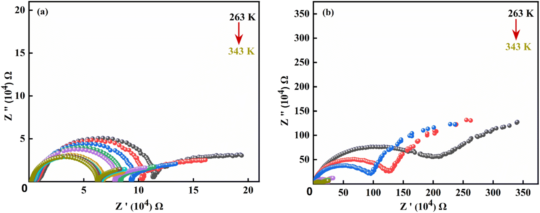Fig. 1 Nyquist plots representing the complex impedance values for the real (Z′) vs. imaginary (Z′′) parts of EIS in a temperature range of 263–343 K for the (a) MAPbI₃ and (2) MAPbBr₃ SCs.

In general, high-frequency spectra stem from the geometrical capacitance and bulk conductivity,^21,22 while low-frequency spectra originate from the ionic phenomena (ion accumulation and transport).²² With an increase in temperature, the radii of the semicircles (low- and high-frequency spectra) of both the SCs decrease somewhat at different rates. For both the SCs, it was observed that with the increase in temperature, the low frequency response nearby (1 Hz) gets shifted towards higher frequencies. A similar behaviour was also observed by Clarke et al. and found that it associated with ionic modulation.²³ This will increase the recombination rate (bulk recombination), which in turn reduces the resistance.²⁴

Fig. S1† illustrates the frequency dependence of the real and imaginary parts of the EIS for both SCs (iodidie and bromide respectively), highlighting their temperature dependence characterstics. Fig. S1(a) and (c)† show the real impedance (Z′) of MAPbI₃ and MAPbBr₃ SCs, revealing a progressive change in slope around the mid-frequency range (kHz). Meanwhile, Fig. S1(b) and (d)† depict the imaginary impedance (Z′′) of both SCs as a function of frequency at different temperatures. In the case of the MAPbI₃ SC, a clear distinct relaxation process at low and high frequencies for each measured temperature is evident. This process is indicative of the time-dependent behaviour of charge carriers. The peak shifts occurred at higher frequencies, with their magnitude decreasing as the temperature increased.²⁵ However, in the case of the MAPbBr₃ SC, maximum change was observed in the mid-frequency range.

To extract the activation energy or electronic and ionic transport phenomena, EIS spectra in the range of low to mid-high temperature are required. Acquisition of EIS spectra at low frequency (less than 10 Hz) as a function of applied temperature and bias together will increase the time of the experiment. For example, in our previous work, we have shown that the time taken to record a single EIS spectrum from 1 MHz to 300 mHz at a particular applied bias was ∼25 min under the given set of parameters.²⁴ In the case of temperature measurements along with the long data acquisition time, a continuous temperature stabilization process is also challenging. Even after the EIS data acquisition, the selection of appropriate circuits, extraction of circuit elements and analysis of the obtained parameters to extract device or material properties conventionally required time from days to months. In addition, the probability of human error can never be ignored.

To minimize experimental acquisition time, analysis time, and human error, we employed machine learning (ML). Specifically, we trained an ML model to predict EIS curves at different temperatures, reducing the need for extensive EIS measurements. To reduce the analysis time and minimize human error, we again utilized ML to analyse the obtained EIS spectra, extract electrical parameters, and perform the necessary fitting to derive material parameters. The selection of the appropriate circuit for the fitting of EIS using ML been adopted from our previous work.¹³

Machine learning analysis and modelling

In this section, we employed ML techniques to develop the model based on the experimental data. The model was designed for uncovering patterns and making precise predictions from the data. The process begins with a comprehensive examination of the dataset along with employing feature engineering methods, followed by the training and evaluation of various models to assess their performance. Subsequently, we selected the most suitable regressor model for the dataset. When selecting the appropriate regressor model, our goal was to ensure that the developed model could perform the following functions: (a) predict the EIS response at various temperatures to assist researchers in conducting EIS measurements at specific temperatures, thereby reducing the overall experimental time; (b) identify the most suitable Electrical Equivalent Circuit (EEC) for fitting the EIS spectra; and (c) utilize the extracted EEC parameters to perform the necessary operations and calculate the material parameters. In the present work, we primarily focused on the calculation of activation energy for perovskite SCs.

Initially, a dataset, consisting of 4648 entries of the EIS spectra of MAPbI₃ and MAPbBr₃ SCs, was developed. The dataset included four key features: temperature, frequency, Re(Z′), and Img(-Z′′). The data for both the SCs were organized in a way so as to maintain the flow of measurements, reflecting the systematic temperature and frequency variations used to capture the real and imaginary impedance components at each step. Additionally, we analyzed the dataset for null, duplicate, and outlier values. While no null or duplicate entries were detected, outliers were identified using boxplots, as shown in Fig. S2.† We found a great deal of outliers in our data set whose presence, if not handled appropriately could affect the model's performance. To handle the outliers and mitigate the effect of the same on the prediction, we employed three mathematical transformations on the frequency feature: square, square-root and logarithmic. Among these, log transformation proved to be the most effective, which significantly reduces outliers. The details of the same, models and mathematical step followed to handle the outliers are discussed in section 3 of the ESI.†

Model training and evaluation

After preparing the dataset for both SCs, the next step is to identify the best algorithm from several regression models. For this, we selected six widely used algorithms such as: Simple Linear Regression (SLR);²⁶ Gradient Boosting Regression (GBR);²⁷ Extreme Gradient Boosting (XGBoost) Regression;²⁸ Random Forest (RF);²⁷ Decision Tree (DT);²⁹ and Gaussian Process Regressor (GPR).³⁰ A subset of the experimental dataset corresponding to five distinct temperatures was completely excluded during the training, validation, and testing phases to ensure it remained entirely hidden from the model during development. The remaining data were split into training, validation, and testing sets, with a ratio of 70% for training, 15% for validation, and 15% for testing. After the model demonstrated strong performance based on the testing and validation metrics, the excluded subset of five temperature spectra was used for additional testing. This process validated the model's ability to generalize effectively to unseen experimental conditions, further strengthening the study's conclusions.

Here, we have made use of Google Colab for implementing the Python code. From the dataset, three features ‘ionic radius’, ‘temperature’, and ‘frequency’ were selected as the input parameters (X), while two features, ‘Re(Z′)’ and ‘Img(-Z′′)’, were chosen as the output parameters (Y). We used sklearn's train_test_split function to divide the X and Y subsets into training, validation, and test sets. This split ensured that we had separate data for training the model, validating its performance and testing its accuracy. The six algorithms under consideration were then trained and subsequently analysed based on their performance.

The dataset was trained using the abovementioned six algorithms to predict the real ‘Re(Z′)’ and imaginary ‘Img(Z′′)’ parts of EIS based on the input features. For performance examination, we used five performance metrics namely, mean squared error (MSE), mean absolute error (MAE), root mean squared error (RMSE), R² score and mean absolute percentage error (MAPE). While MAE, MSE, RMSE, and MAPE are categorized as error metrics, the R² score is regarded as a relative metric. The performance comparison based on three of the above-mentioned error metrics (MAE, MSE, RMSE) on the train data is shown in Fig. 2(a) for selected regression algorithms. It was found that for DT, error values reduced to zero are overfitting, rendering it unsuitable for use. In contrast, the remaining algorithms warrant consideration for performance evaluation on validation data.

Fig. 2 (a) Performance comparison of different regression algorithms based on the trained data. Comparison of the actual and predicted Nyquist plots using RF regressor at 333 K for (b) MAPbBr₃ and (c) MAPbI₃. Fitted Nyquist plots based on the predicted data at 333 K for (d) MAPbBr₃ and (e) MAPbI₃.

Following this, GBR, RF and XGBoost Regression turned out as the three best performing algorithms among others, based on their results on validation data. To further improve the performance of the selected algorithms, we applied hyperparameter tuning on the same, and eventually compared the tuned models’ performance on the test data. Here, we used the GridSearchCV method, which is one of several available tuning techniques. This final review revealed RF to be the best algorithm, outperforming the other two algorithms, prompting us to proceed with this regression method. The RF algorithm generally outperforms others due to its robustness against noise. It builds multiple independent decision trees and averages their outputs, reducing the impact of dataset variations.³¹ In contrast, GBR and XGBoost Regression are more sensitive to noise as they sequentially correct errors, which can amplify the effects of outliers.³² RF also requires fewer hyperparameters to tune, especially when the data are clean. Its ensemble approach, where multiple trees are trained on random subsets, makes it effective for moderate-sized datasets without overfitting.^31,33 Unlike boosting methods optimized for large datasets and parallel processing, RF has lower computational demands, making it ideal for moderate datasets like this.³⁴ The performance comparison of the chosen model based on three performance metrics, MSE, MAE and RMSE, as well as a table representing the tuned parameters of the same, is provided in Fig. S4 and Table S1,† respectively. As mentioned above, we didn't use a subset of the dataset for the selection of the best model. This subset included data at five distinct temperatures: 268 K, 293 K, 298 K, 328 K, and 333 K. This entire dataset was unseen for the selected algorithm and was fully utilized for the prediction tasks. Initially, this small dataset (subset of the dataset) was subjected to a similar feature engineering process as discussed in the above section to make it ready for prediction. The input and output parameters are separated as discussed previously. The tuned RF model, which eventually came out to be the best-performing model as mentioned above, was utilized to predict the output features. The predictions were subsequently scaled back to their original values and compared with the actual data to assess the model's accuracy. The predictions for the other temperatures for both the SCs are shown in Fig. S5.†

To obtain the useful information from the EIS spectra, it is crucial to extract the resistive and capacitive components with the help of an EEC. Conventionally in practice, extraction of the circuit element evolves identification of the EEC followed by simulation of the EEC via software or by running the codes in MATLAB or Excel. Fig. 2(d) and (e) illustrate the fitted Nyquist plot for MAPbBr₃ and MAPbI₃ SCs at 333 K after adjusting initial parameters to achieve the best fit which are shown in Tables S3 and S4† respectively. Similarly, fitting of Nyquist plots and parameter extraction of MAPbI₃ at 268 K, 293 K, 298 K, and 328 K are shown in Fig. S6 and Tables S5–S8.† Here, an iterative fitting process was employed with the help of the developed ML model. The selection of the appropriate EEC among the widely available EECs, frequency range and iteration time is wisely decided by the developed ML model which is discussed in detail in our previous work.¹³ In the present case, the ML model chosen two RC pairs with series resistance. The extracted electrical parameters were refined to achieve the best possible match between the model and the experimental data for both MAPbBr₃ and MAPbI₃ SCs.²⁵

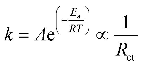
The developed ML model discussed in our previous work¹³ was further upgraded to analyze the extracted electrical parameters of EEC and to calculate the activation energy. The activation energy was calculated using an automated analyzer tool, which processes the circuit elements extracted from the fitted equivalent circuits (ECs) of the EIS spectra. These circuit elements are used to compute activation energy values based on their temperature dependence, following established electrochemical principles. The calculated values were validated against the literature, ensuring accuracy and consistency. The activation energy (E_a) is directly related to the rate of charge transfer within the crystal.^35,36 To calculate the activation energy, the low-frequency resistance values (R_ct) of both SCs were considered. The charge transfer resistance (R_ct) represents resistance to charge migration and its reciprocal (1/R_ct) is proportional to the rate of charge transfer across the crystal. The equation used for the calculations is as follows:³⁷

where k is the rate constant of an electrochemical process, R_ct is the charge transfer resistance, A is the pre-exponential factor, E_a is the activation energy, R is the gas constant, and T is the temperature. Charge transfer resistance values are extracted through a Python pipeline script for equivalent circuit fitting.

The Arrhenius equation can be written in the logarithmic form to justify this use, as seen below:

As observed from eqn (2), to calculate the activation energy, we plotted ln(1/R_ct) obtained from the EIS spectra fitting versus 1000/T (in Kelvin).

Fig. 3 shows the software-generated linear fitting of the Arrhenius plots obtained for MAPbBr₃ and MAPbI₃ SCs having R² scores of 0.8485 and 0.6393 with the extracted activation energy values of 0.25 and 0.32 eV respectively. The obtained values of activation energy for both the SCs are the same as the values reported by other authors and in our previous studies.^6,11,38,39

Fig. 3 Arrhenius plot representing the linearity curve with slops derived using the experimental data for (a) MAPbBr₃ and (b) MAPbI₃, respectively.

3. Conclusion

The present study focuses on the utilization of ML to automate EIS data acquisition, predicting EIS spectra at unknown temperatures, fitting the appropriate electrical circuit, and automatically extracting passive component values to calculate the activation energy via an Arrhenius plot for MHP SCs. Our developed ML model is capable of predicting the EIS spectra for unknown temperature values, thereby reducing the data acquisition time significantly. Moreover, the developed ML model reduces the human error by automating the extraction of electrical parameters and performs the needed fitting from the obtained EIS spectra. Here, the ML-based model extracted activation energy values of 0.25 and 0.32 eV for the MAPbBr₃ and MAPbI₃ SCs which are comparable to our previous work and studies by other authors. The results highlight the potential of ML to automate the EIS acquisitions and analysis in a more convenient and efficient way.

Author contributions

VM, KS, and KU developed the codes. RDP performed the experiments and formulated the ML studies. SVP and AK helped with the initial draft and experimental studies. DP, SA, and PY supervised the project.

Data availability

The codes and utilized dataset can be easily found within the GitHub repository of KU, https://github.com/kushal-unjiya/EIS-Electrochemical-Impedance-Spectroscopy.

On behalf of all the authors PY confirm that the needed informations and required data are available in the main manuscript and the ESI.† Any additional data to support the objectives can also be provided upon request.

Conflicts of interest

The authors declare no conflict of interest.

Acknowledgements

P. Y. acknowledges the ORSP of Pandit Deendayal Energy University and DST SERB (IPA/2021/96) for the financial support. A. K. is thankful to the Dean of Scientific Research, King Khalid University for financial support by grant number RGP 2/345/45. PY also acknowledges Mr Pawan for helping in the initial experiments.

References

1. X.-K. Liu, W. Xu, S. Bai and Y. Jin, et al., Metal halide perovskites for light-emitting diodes, Nat. Mater., 2021, 20(1), 10–21.
2. H. Jin, E. Debroye, M. Keshavarz and I. G. Scheblykin, et al., It's a trap! On the nature of localised states and charge trapping in lead halide perovskites, Mater. Horiz., 2020, 7(2), 397–410.
3. D. Duan, C. Ge, M. Z. Rahaman and C.-H. Lin, et al., Recent progress with one-dimensional metal halide perovskites: from rational synthesis to optoelectronic applications, NPG Asia Mater., 2023, 15(1), 8.
4. X. Fu, M. Wang, Y. Jiang and X. Guo, et al., Mixed-Halide Perovskites with Halogen Bond Induced Interlayer Locking Structure for Stable Pure-Red PeLEDs, Nano Lett., 2023, 23(14), 6465–6473.
5. S. Min, H. Choe, S. H. Jung and J. Cho, How Chemical Bonding Impacts Halide Perovskite Nanocrystals Growth to Bulk Films: Implication of Pb–X Bond on Growth Kinetics, ChemPhysChem, 2023, 24(14), e202300202.
6. S. Yang, S. Chen, E. Mosconi and Y. Fang, et al., Stabilizing halide perovskite surfaces for solar cell operation with wide-bandgap lead oxysalts, Science, 2019, 365(6452), 473–478.
7. W. Zhou, X. Chen, R. Zhou and H. Cai, et al., The Role of Grain Boundaries on Ion Migration and Charge Recombination in Halide Perovskites, Small, 2024, 20(32), 2310368.
8. S. P. Senanayak, K. Dey, R. Shivanna and W. Li, et al., Charge transport in mixed metal halide perovskite semiconductors, Nat. Mater., 2023, 22(2), 216–224.
9. L. Zuo, Z. Li and H. Chen, Ion Migration and Accumulation in Halide Perovskite Solar Cells, Chin. J. Chem., 2023, 41(7), 861–876.
10. M. Bag, L. A. Renna, R. Y. Adhikari and S. Karak, et al., Kinetics of Ion Transport in Perovskite Active Layers and Its Implications for Active Layer Stability, J. Am. Chem. Soc., 2015, 137(40), 13130–13137.
11. A. Mahapatra, R. Runjhun, J. Nawrocki and J. Lewiński, et al., Elucidation of the role of guanidinium incorporation in single-crystalline MAPbI ₃ perovskite on ion migration and activation energy, Phys. Chem. Chem. Phys., 2020, 22(20), 11467–11473.
12. M. T. Khan, A. Almohammedi, S. Kazim and S. Ahmad, Electrical Methods to Elucidate Charge Transport in Hybrid Perovskites Thin Films and Devices, Chem. Rec., 2020, 20(5), 452–465.
13. S. Kadiwala, S. V. Pandey, D. Purohit and D. Hirpara, et al., In-Line Electrochemical Impedance Spectroscopy for Real-Time Circuit Identification and Interpretation in Metal Halide Perovskite Single Crystals, J. Phys. Chem. C, 2024, 128(23), 9776–9784.
14. N. Filipoiu, A. T. Preda, D.-V. Anghel and R. Patru, et al., Capacitive and Inductive Effects in Perovskite Solar Cells: The Different Roles of Ionic Current and Ionic Charge Accumulation, Phys. Rev. Appl., 2022, 18(6), 64087.
15. A. J. Riquelme, K. Valadez-Villalobos, P. P. Boix and G. Oskam, et al., Understanding equivalent circuits in perovskite solar cells. Insights from drift-diffusion simulation, Phys. Chem. Chem. Phys., 2022, 24(26), 15657–15671.
16. S. V. Pandey, D. Prochowicz, A. Mahapatra and S. Pandiaraj, et al., The circuitry landscape of perovskite solar cells: An in-depth analysis, J. Energy Chem., 2024, 94, 393–413.
17. N. Parikh, S. Akin, A. Kalam, D. Prochowicz and P. Yadav, Probing the Low-Frequency Response of Impedance Spectroscopy of Halide Perovskite Single Crystals Using Machine Learning, ACS Appl. Mater. Interfaces, 2023, 15(23), 27801–27808.
18. S. V. Pandey, N. Parikh, A. Mahapatra and A. Kalam, et al., Deconvoluting the Impedance Response of Halide Perovskite Single Crystals: The Distribution of Relaxation Time Method, J. Phys. Chem. C, 2023, 127(24), 11609–11615.
19. N. K. Tailor, A. Mahapatra, A. Kalam and M. Pandey, et al., Influence of the A-site cation on hysteresis and ion migration in lead-free perovskite single crystals, Phys. Rev. Mater., 2022, 6(4), 45401.
20. R. Saraf, A. Mathur and V. Maheshwari, Polymer-Controlled Growth and Wrapping of Perovskite Single Crystals Leading to Better Device Stability and Performance, ACS Appl. Mater. Interfaces, 2020, 12(22), 25011–25019.
21. J. Bisquert and A. Guerrero, Chemical Inductor, J. Am. Chem. Soc., 2022, 144(13), 5996–6009.
22. E. Guillén, F. J. Ramos, J. A. Anta and S. Ahmad, Elucidating Transport-Recombination Mechanisms in Perovskite Solar Cells by Small-Perturbation Techniques, J. Phys. Chem. C, 2014, 118(40), 22913–22922.
23. W. Clarke, G. Richardson and P. Cameron, Understanding the Full Zoo of Perovskite Solar Cell Impedance Spectra with the Standard Drift–Diffusion Model, Adv. Energy Mater., 2024, 14(32), 2400955.
24. N. S. Hill, M. V. Cowley, N. Gluck and M. H. Fsadni, et al., Ionic Accumulation as a Diagnostic Tool in Perovskite Solar Cells: Characterizing Band Alignment with Rapid Voltage Pulses, Adv. Mater., 2023, 35(32), 2302146.
25. W. Clarke, P. Cameron and G. Richardson, The effects of device degradation on perovskite solar cell impedance spectra: insights from a drift-diffusion model, 2024.  DOI:10.26434/chemrxiv-2024-2tbm9.
26. S. Weisberg, Applied Linear Regression.
27. J. H. Friedman, Greedy function approximation: A gradient boosting machine, Ann. Stat., 2001, 29(5), 1189–1232.
28. T. Chen and C. Guestrin, XGBoost, in Proceedings of the 22nd ACM SIGKDD International Conference on Knowledge Discovery and Data Mining, ACM, 2016, pp. 785–794.
29. Y.-Y. Song and Y. Lu, Decision tree methods: applications for classification and prediction, Shanghai Arch. Psychiatry, 2015, 27(2), 130–135.
30. C. K. I. Williams and C. E. Rasmussen, Gaussian Processes for Regression.
31. L. Breiman, Random Forests. Machine Learning, Mach. Learn., 2001, 45(1), 5–32.
32. C. Bentéjac, A. Csörgő and G. Martínez-Muñoz, A Comparative Analysis of XGBoost, 2019.  DOI:10.48550/arXiv.1911.01914.
33. E. Halabaku and E. Bytyçi, Overfitting in Machine Learning: A Comparative Analysis of Decision Trees and Random Forests, Intell. Autom. Soft Comput., 2024, 39(6), 987–1006.
34. T. Chen and C. Guestrin, XGBoost, in Proceedings of the 22nd ACM SIGKDD International Conference on Knowledge Discovery and Data Mining, ACM, New York, NY, USA, 2016, pp. 785–794.
35. A. Mahapatra, D. Prochowicz, J. Kruszyńska and S. Satapathi, et al., Effect of bromine doping on the charge transfer, ion migration and stability of the single crystalline MAPb(Br_xI_1−x)₃ photodetector, J. Mater. Chem. C, 2021, 9(42), 15189–15200.
36. L. McGovern, I. Koschany, G. Grimaldi, L. A. Muscarella and B. Ehrler, Grain Size Influences Activation Energy and Migration Pathways in MAPbBr ₃ Perovskite Solar Cells, J. Phys. Chem. Lett., 2021, 12(9), 2423–2428.
37. A. Mavlonov, Y. Hishikawa, Y. Kawano and T. Negami, et al., Thermal stability test on flexible perovskite solar cell modules to estimate activation energy of degradation on temperature, Sol. Energy Mater. Sol. Cells, 2024, 277, 113148.
38. C. Eames, J. M. Frost, P. R. F. Barnes and B. C. O'Regan, et al., Ionic transport in hybrid lead iodide perovskite solar cells, Nat. Commun., 2015, 6(1), 7497.
39. L. McGovern, M. H. Futscher, L. A. Muscarella and B. Ehrler, Understanding the Stability of MAPbBr ₃ versus MAPbI₃: Suppression of Methylammonium Migration and Reduction of Halide Migration, J. Phys. Chem. Lett., 2020, 11(17), 7127–7132.

---

Footnote

† Electronic supplementary information (ESI) available: Section 1 includes synthesis of MHPSCs and computational analysis aspect. Section 2 includes temperature-dependent EIS spectra of MAPbI₃ and MAPbBr₃ as a function of frequency. Section 3 shows feature engineering data visualization plots. Section 4 shows training and validation set performance of actual vs. predicted datasets and hyperparameters of model and performance metrics. Section 5 gives information about fitted Nyquist plots and parameter extraction at unseen temperatures. See DOI: https://doi.org/10.1039/d4dt03123g

---