 Open Access Article
Machine learning of optical properties of materials – predicting spectra from images and images from spectra†
Helge S.
Stein
 *,
Dan
Guevarra
,
Paul F.
Newhouse
,
Edwin
Soedarmadji
and
John M.
Gregoire
 *
*
Joint Center for Artificial Photosynthesis, California Institute of Technology, Pasadena, California 91125, USA. E-mail: stein@caltech.edu; gregoire@caltech.edu
First published on 25th October 2018
Abstract
As the materials science community seeks to capitalize on recent advancements in computer science, the sparsity of well-labelled experimental data and limited throughput by which it can be generated have inhibited deployment of machine learning algorithms to date. Several successful examples in computational chemistry have inspired further adoption of machine learning algorithms, and in the present work we present autoencoding algorithms for measured optical properties of metal oxides, which can serve as an exemplar for the breadth and depth of data required for modern algorithms to learn the underlying structure of experimental materials science data. Our set of 178![[thin space (1/6-em)]](https://www.rsc.org/images/entities/char_2009.gif) 994 distinct materials samples spans 78 distinct composition spaces, includes 45 elements, and contains more than 80
994 distinct materials samples spans 78 distinct composition spaces, includes 45 elements, and contains more than 80![[thin space (1/6-em)]](https://www.rsc.org/images/entities/char_2009.gif) 000 unique quinary oxide and 67
000 unique quinary oxide and 67![[thin space (1/6-em)]](https://www.rsc.org/images/entities/char_2009.gif) 000 unique quaternary oxide compositions, making it the largest and most diverse experimental materials set utilized in machine learning studies. The extensive dataset enabled training and validation of 3 distinct models for mapping between sample images and absorption spectra, including a conditional variational autoencoder that generates images of hypothetical materials with tailored absorption properties. The absorption patterns auto-generated from sample images capture the salient features of ground truth spectra, and band gap energies extracted from these auto-generated patterns are quite accurate with a mean absolute error of 180 meV, which is the approximate uncertainty from traditional extraction of the band gap energy from measurements of the full transmission and reflection spectra. Optical properties of materials are not only ubiquitous in materials applications but also emblematic of the confluence of underlying physical phenomena yielding the type of complex data relationships that merit and benefit from neural network-type modelling.
000 unique quaternary oxide compositions, making it the largest and most diverse experimental materials set utilized in machine learning studies. The extensive dataset enabled training and validation of 3 distinct models for mapping between sample images and absorption spectra, including a conditional variational autoencoder that generates images of hypothetical materials with tailored absorption properties. The absorption patterns auto-generated from sample images capture the salient features of ground truth spectra, and band gap energies extracted from these auto-generated patterns are quite accurate with a mean absolute error of 180 meV, which is the approximate uncertainty from traditional extraction of the band gap energy from measurements of the full transmission and reflection spectra. Optical properties of materials are not only ubiquitous in materials applications but also emblematic of the confluence of underlying physical phenomena yielding the type of complex data relationships that merit and benefit from neural network-type modelling.
Introduction
Recent advances in computer science1–4,38 enable materials scientists to predict new properties,2 generate entirely new materials,5 and identify reaction pathways.6 Illustrative examples of predictive machine learning models in materials science include the prediction of optical and electrical properties based on representations of crystal structures as fragments7–9 and the prediction of materials with complex electronic structures such as thermoelectrics10 or organic light emitting diodes.11 These successful implementations of modern machine learning algorithms are mostly limited to theoretical (i.e. computational) data, leaving an open question as to whether such algorithms can be impactful in materials science experiments. Many machine learning algorithms require diverse, expansive training datasets, limiting their adoption in experimental materials science where such data is generally not available. High-throughput materials science12–17 can help address these data scarcity issues, as demonstrated by Zakutayev et al.18 with their utilization of high throughput experiment data to train a random forest model that predicts electrical resistivity from material composition using 16![[thin space (1/6-em)]](https://www.rsc.org/images/entities/char_2009.gif) 093 distinct materials. While there exists a variety of algorithms for machine learning in low data regimes (<103 samples), which to date have been primarily applied in organic chemistry,19–23 meaningful exploration and prediction in the breadth of materials compositions offered by the periodic table will most likely require significantly larger datasets.
093 distinct materials. While there exists a variety of algorithms for machine learning in low data regimes (<103 samples), which to date have been primarily applied in organic chemistry,19–23 meaningful exploration and prediction in the breadth of materials compositions offered by the periodic table will most likely require significantly larger datasets.
Among the materials science machine learning algorithms reported to date, random forest models are commonly used, which is understandable given their predictive power, but the lack of interpretability of this and other machine learning models limit their ability to generate new materials knowledge. Design of materials with tailored properties is central to materials research, and machine learning-based acceleration of materials design was demonstrated by Gómez-Bombarelli et al.5 through development of a conditional variational autoencoders (cVAE) that predicts new organic molecules based on user-specified properties. Variational autoencoders (VAE)24 and cVAEs25 utilize neural networks, whose deployment in materials science can enable new modes of scientific discovery through exploration of the latent space to reveal new and previously unknown relationships.26 Our quest to develop models that learn the underlying structure of experimental materials data has resulted in the development of a VAE and cVAE to predict optical absorption spectra from images of materials, and images from user-tailored absorption spectra.
Our focus on optical characterization data is motivated by the importance of optical properties for a broad span of technologies, from computer displays to solar energy utilization.27 The data employed in the present work results from years of extensive materials synthesis and optical characterization using a fixed set of high throughput instruments in the Joint Center for Artificial Photosynthesis.28,29 Optical characterizations utilizing inexpensive commercial sensors are particularly amenable to high throughput experimentation, making coarse optical characterization of new materials more expedient by experiment than by computation, particularly due to the high computational expense for predicting optical properties like band gap energy at reasonable accuracy; state of the art hybrid functionals require several CPU hours per material to achieve a bandgap prediction RMSE of 0.74 eV for metal oxide materials.30 The recently reported machine learning model by Oses et al.7 achieves an RMSE of 0.51 eV for computationally-predicted band gaps, which improves band gap prediction but not band gap measurement. Recently published algorithms have automated the extraction of band gap energy from an ultraviolet-visible (UV-vis) optical absorption spectrum,30,31 leaving spectrum acquisition as the rate limiting step of band gap measurement. As a result, the prediction of absorption spectra from a higher throughput experimental technique, such as imaging with a consumer product, would be quite impactful. We demonstrate machine learning automation of this task by combining a VAE with a deep neural network, requiring only an image of the material as input. We also exploit machine learning of the relationships between image and absorption spectrum to create a predictive model for the image of a material with tailored optical absorption properties, which is the first generative model5,19 trained exclusively from experimental materials data.
Results and discussion
Design and training of machine learning models
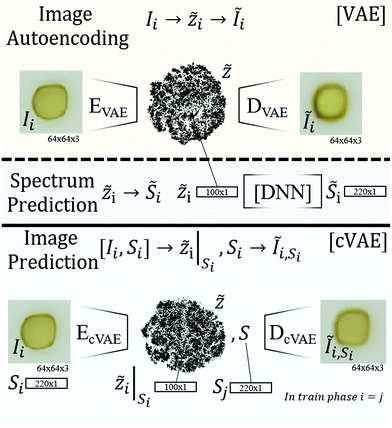
At a high level, imaging a material with a standard sensor, such as a red-green-blue (RGB) complementary metal oxide semiconductor (CMOS) sensor, is a spatially resolved measurement of an optical property averaged over some spectral range, including some spectral overlap of the 3 color filters.32 The optical property being measured is an unknown combination of reflection, absorption and transmission properties, which is complementary to a spectral optical absorption measurement that averages over a sample region (lower spatial resolution) but uses spectrometers to attain high energy (wavelength) resolution. The standard spectral absorption technique also employs distinct transmission and reflection measurements from which the spectral absorption can be modelled. The inability to derive a first-principles transformation between these 2 types of optical data arises from the unknown relationship between the RGB image and absorption, and unknown mapping from the broad spectral response of each CMOS channel to the high energy resolution of an absorption spectrum, which in the present case is 220 energies between 1.31 and 3.1 eV. Deriving such a mapping would be facilitated by a low-parameter functional form for how absorption varies with energy in metal oxide materials, but such a model is not forthcoming due to the various types of absorption phenomena and the mixing of absorption signals from multiple phases in the typically mixed-phase metal oxide samples. Consequently, machine learning of the underlying data relationships is the only viable option. Predicting absorption spectra from images is thus only possible if a machine learning algorithm can exploit “hidden” information in the high spatial-resolution images, i.e. patterns unbeknownst to expert materials scientists.Our exploration of the ability of machine learning to model complex relationships in materials data proceeded through the development of 3 models (Fig. 1) with training and validation data extracted from a set of 180![[thin space (1/6-em)]](https://www.rsc.org/images/entities/char_2009.gif) 902 images and spectra, including 1908 “blank” samples (nothing deposited on the substrate) and 178
902 images and spectra, including 1908 “blank” samples (nothing deposited on the substrate) and 178![[thin space (1/6-em)]](https://www.rsc.org/images/entities/char_2009.gif) 994 metal oxide samples synthesized via inkjet printing of mixed elemental precursors followed by thermal processing in an O2-containing atmosphere. The metal oxides samples contain various combinations of 1 to 4 cation elements along with various inkjet printing and thermal processing parameters, and while these important metadata are included in the dataset, they are not used in the models describe herein.
994 metal oxide samples synthesized via inkjet printing of mixed elemental precursors followed by thermal processing in an O2-containing atmosphere. The metal oxides samples contain various combinations of 1 to 4 cation elements along with various inkjet printing and thermal processing parameters, and while these important metadata are included in the dataset, they are not used in the models describe herein.
In the present work, the absorption spectrum of a sample is taken to be the product of the spectral absorption coefficient and the sample thickness, which is a unitless quantity and the standard output from spectral absorption measurements. The thickness of the inkjet printed samples are on the order of 100 nm, so an absorption spectrum value of 1 corresponds to an absorption coefficient on the order of 105 cm−1. As previously described,23 the inkjet printed samples are rough over multiple length scales, further complicating the relationship between images and absorption spectra. The discrete samples are deposited over approximately 1 mm2 of the glass substrate with a 2 mm sample pitch. Each sample image is automatically cropped from the image of the entire library of materials on the glass substrate, and each 2.1 mm × 2.1 mm sample image is sufficiently large to cover the extent of each material with a border of bare substrate.
Model 1 – variational autoencoder
To establish the appropriate methods for encoding images of metal oxides, we commenced with the design and training of model 1, an autoencoder for flatbed scanner images of materials synthesized by the inkjet printing technique. An autoencoder takes an input (here an image of a material) and encodes it into a latent space of lower dimension (here 100 dimensions). Decoding a latent space coordinate produces an image in the same format as the input data, making the process akin to lossy compression, and the latent space (compressed) representation can enable new analyses and algorithms. Models employing convolutional layers19 excel at reconstructing sample morphology and were thus employed in model 1, requiring hyperparameter optimization as described below.Model 2 – prediction of UV-vis spectra
The Absorption Spectra Prediction Model (ASPM) builds upon the compact latent space representation of the VAE to predict a UV-vis absorption spectrum (220 energies). Under the assumption that the image encoder captures various image properties such as the color, color variation, morphology, etc. in its latent space representation, this approach exploits the high information density of the latent space (100 dimensions compared to the 12![[thin space (1/6-em)]](https://www.rsc.org/images/entities/char_2009.gif) 288 dimensions of the 64 × 64 RGB image) for the construction of absorption spectra, in this case using a hybrid dense and convolutional deep neural network model that was trained independently from model 1.
288 dimensions of the 64 × 64 RGB image) for the construction of absorption spectra, in this case using a hybrid dense and convolutional deep neural network model that was trained independently from model 1.
Model 3 – conditional variational autoencoder
The conditional Variational Autoencoder (cVAE) follows the general structure of the VAE with modified inputs for both the encoding and decoding algorithms. The encoder input is the concatenation of the flattened image and absorption spectrum, and the decoder input is the concatenation of the latent space coordinate and the conditional absorption spectrum so that the resulting image represents the latent space coordinate under the condition that the material exhibits the specified ‘conditional’ absorption spectrum. During training, the same absorption spectrum was used in the encoder and decoder inputs as noted in Fig. 1. During application of the model (conditional decoding), the conditional absorption spectrum was user-specified as described below.Image autoencoding and spectral prediction
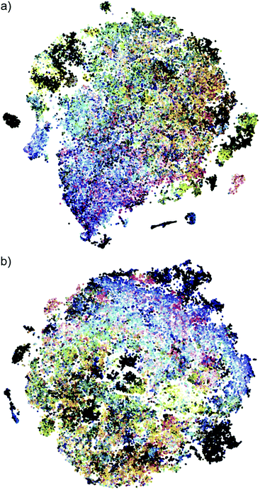
The VAE of model 1 was trained for 100 epochs after training hyperparameters including the number of filters in the convolutional layers and latent space dimensions, as shown in the ESI.† Using t-distributed stochastic neighbor embedding (t-SNE),33 the 100-dimensional latent space can be visualized as shown in Fig. 2a for the 54![[thin space (1/6-em)]](https://www.rsc.org/images/entities/char_2009.gif) 270 images of test set, where each sample point is plotted using its representative color (see figure caption). Even though the VAE was not supplied any spectral information, it inherently exploits spectral features during autoencoding, as evident from the black-brown to blue-purple color gradient from left to right. The apparent clustering of samples, particularly those with a similar representative color, is emblematic of the structuring in the latent space based on optical properties.
270 images of test set, where each sample point is plotted using its representative color (see figure caption). Even though the VAE was not supplied any spectral information, it inherently exploits spectral features during autoencoding, as evident from the black-brown to blue-purple color gradient from left to right. The apparent clustering of samples, particularly those with a similar representative color, is emblematic of the structuring in the latent space based on optical properties.
Example raw (Ii) and VAE-reconstructed (IĨi) images are shown in Fig. 3, demonstrating that the general appearance and especially the human-perceived color of the materials is well reconstructed, however with some additional blurring that occurs in image autoencoding with dimensionality of the latent space well below that of the images.24,25 Since an absorption spectrum is measured with illumination of the entire sample, yielding the spatially “averaged” absorption signal, this blurriness of the reconstructed images is not important for the present purposes, but it is worth noting that the presence of a so-called coffee ring35 in Ii typically results in a darker edge of the sample blob in IĨi. The VAE preservation of perceived color (Fig. 3) and color-based clustering in the latent space (Fig. 2a) indicate that the VAE successfully encoded spectral features even though the model was not supplied any spectral information, motivating the use of latent space representations for predicting spectral absorption.
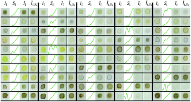 | ||
| Fig. 3 Reconstruction comparison from VAE and cVAE of randomly selected images from the test set. There are 5 large columns of images separated by thick black lines, and within each of these the 4 columns of data are the measured image, measured absorption spectrum, VAE-reconstructed image, and cVAE-reconstructed image, respectfully. Both models successfully reconstruct the apparent color of the original image and aspects of the morphology (such as presence of a “coffee ring”35). Histograms of the cross entropy loss between reconstructed and measured images and for the MSE loss between predicted and measured absorption spectra are shown in Fig. S5 and S6.† | ||
Absorption spectrum prediction
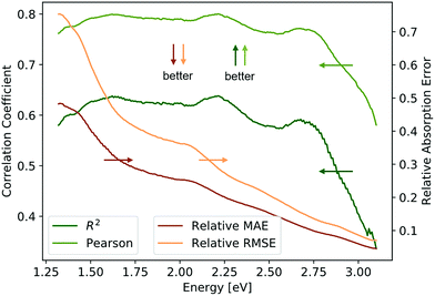
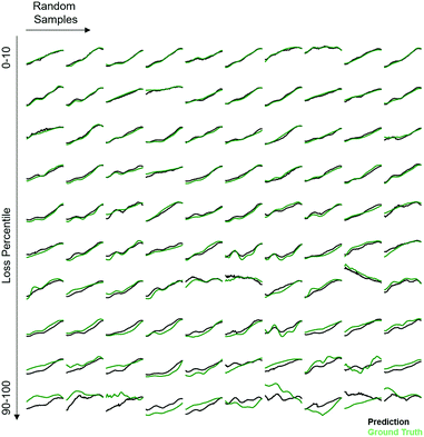
The Absorption Spectra Prediction Model (ASPM) was trained and validated using the VAE latent space coordinates, with the same train-test split used in model 1. The weights of the VAE of model 1 were no longer trainable at this stage. Overall, there was good convergence for the ASPM across the energy range of the absorption spectra as shown in Fig. 4. The relatively high and consistent R2 and Pearson correlation coefficients together with low residual losses demonstrate that at each energy value, the measured absorption spectra are well-reconstructed by model 2. Visual inspection of the absorption spectrum prediction for a span of representative samples is shown in Fig. 5 that compares ground truth absorption spectra (green) from the test set and their prediction (black) from model 2. The figure includes a row of plots from each loss decile, with ten randomly selected samples in each row. For up to the 80th loss percentile, the predicted spectra appear in good agreement with the ground truth spectra. Impressively, the model reconstructs fine features of the absorption spectra such as local maxima that result from sub-band gap absorption or thin-film interference, even when these features occur over spectral ranges much smaller than the sensitivity range of the original RGB sensor. Even an expert materials scientist cannot identify the presence of such features from inspection of an image, demonstrating the super-human analysis capabilities of these machine learning models.The quality of the predicted UV-vis spectra allows their utilization for estimating band gap energy, which is typically a manual human analysis exercise but has recently been automated to identify a representative band gap energy for a given absorption spectrum.31,34 As most of the herein studied materials are multiphase materials (due to their high computational order) it should be noted that the MARS algorithm employed here returns only a single representative band gap energy without a measure of uncertainty. For each sample i, the performance of model 2 for band gap estimation is thus evaluated by comparing the MARS-identified direct band gap energy from the ground truth spectra Si to that from the predicted spectra ![[S with combining tilde]](https://www.rsc.org/images/entities/i_char_0053_0303.gif) i, as summarized in Fig. 6 for the test set. The mean band gap error is −10 meV (median 8.8 meV); the root mean squared error is 261 meV; and the mean absolute error is 180 meV. The prediction of band gaps based on the latent space representation of images therefore outperforms the ab initio calculations noted above by extracting knowledge from the coarse optical characterization data in the flatbed scanner images.
i, as summarized in Fig. 6 for the test set. The mean band gap error is −10 meV (median 8.8 meV); the root mean squared error is 261 meV; and the mean absolute error is 180 meV. The prediction of band gaps based on the latent space representation of images therefore outperforms the ab initio calculations noted above by extracting knowledge from the coarse optical characterization data in the flatbed scanner images.
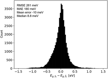 | ||
Fig. 6 Difference between the band gap energy extracted from the experimentally measured spectrum (Si) and from the absorption spectrum produced by model 2 (![[S with combining tilde]](https://www.rsc.org/images/entities/i_char_0053_0303.gif) i), which was predicted using only the image of the material. For both types of spectra, the band gap energy was calculated using the recently-reported MARS based segmentation model.31 i), which was predicted using only the image of the material. For both types of spectra, the band gap energy was calculated using the recently-reported MARS based segmentation model.31 | ||
Conditional variational autoencoder
A complementary demonstration of the ability of machine learning models to encode materials properties is the development of a generative model that makes predictions of materials data from user-specified properties. For this purpose, the cVAE of model 3 was designed to predict how a printed material looks like based on a target absorption spectrum. From visual inspection of reconstructed images using the experimental image and spectrum as input the cVAE performs relatively similar to the VAE.To generate conditionally decoded images, we used a random sample from the test set and identified its latent space coordinate ![[Z with combining tilde]](https://www.rsc.org/images/entities/i_char_005a_0303.gif) i. From this fixed point in the cVAE latent space, various tailored absorption spectra were applied as the conditional input to the decoder, resulting in cVAE-generated images of hypothetical materials as shown in Fig. 7.
i. From this fixed point in the cVAE latent space, various tailored absorption spectra were applied as the conditional input to the decoder, resulting in cVAE-generated images of hypothetical materials as shown in Fig. 7.
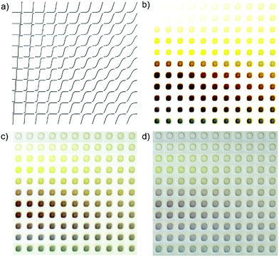 | ||
| Fig. 7 Demonstration of image prediction from an absorption spectrum using model 3 (cVAE). The array of synthetic absorption patterns are generated from the sigmoid function with transition energy increasing from bottom row (1.36 eV) to top (2.9 eV) row and transition width increasing from left column to right column as shown schematically in (a). Each spectrum is additionally modified to obtain maximum absorption values of (b) 2.0, (c) 0.75, (d) 0.25 in the absorption spectrum Si to simulate thicker (strongly absorbing) to thinner (weakly absorbing) materials. Each predicted material image originated from the same randomly chosen latent space coordinate (see Fig. S6† for different latent space coordinates) and thus differ only by the respective conditional spectrum provided to the decoder DcVAE. Conditionally predicted images based on a single latent space point using the conditional absorption spectra shown in (a). Going down in the matrix corresponds to a lower band gap, going right to a lower slope of the sigmoid or less steep absorption factor. Given the gray appearance of the substrate (see Fig. 3 and S1†) samples with lower values in Sj appear more gray (less color saturation). Given the general rule of thumb of yellow-transparent high bandgap materials and brown-red-blue lower bandgap materials a reasonable prediction is achieved. | ||
To generate a series of synthetic absorption spectra that each represent a semiconductor's absorption edge, a sigmoid function was used with variation of the inflection point energy (representing absorption edge energy, increasing from bottom to top in Fig. 7a) and the slope (representing sharpness of absorption increase, decreasing from left to right in Fig. 7a). Application of the MARS algorithm to this series of absorption patterns results in band gap variation of approximately 1.4 to 2.9 eV. To model different material thickness or maximum absorption coefficient, this family of synthetic absorption spectra was scaled to maximum values of 0.84, 0.42, and 0.21 for image generation in Fig. 7b–d, respectively. The highest absorption factor measured in the test set was 0.75, making the generated images in Fig. 7b an extension beyond the span of absorption spectra in the train set. Fig. 7b is commensurate with the general observation of metal oxide semiconductors that a material with a high band gap typically appears yellowish-transparent (e.g. BiVO4 with 2.5 eV band gap), a material with an intermediate band gap appears red-brown (e.g. Fe2O3 with 2.2 eV band gap), and a material with very low band gap appears blue-grey (e.g. Si with 1.2 eV band gap). The apparent transparency and saturation of the generated images is also quite intuitive as high absorption values and low sigmoid slopes that correspond to absorption over a broad spectral range lead to high opacity and low color saturation. With lower maximum absorption, the center part of each image tends to become grayer, which is assumed to be the model's simulation of transparency given the gray appearance of the substrate/background in the flatbed scanner images. High absorption slope in the conditional spectra results in slightly increased sample size in the decoded image, likely due to the network trying to match the absorption condition by making the absorbing part of the image larger, an unintended but interesting mechanism by which the conditional spectrum impacts shapes in the generated image.
To ascertain the relative insensitivity of the generated image to the starting latent space coordinate, Fig. S6† shows a series of images using the conditional spectra from Fig. 7b and 200 ![[Z with combining tilde]](https://www.rsc.org/images/entities/i_char_005a_0303.gif) i values from randomly chosen samples. The ability to generate simulated data for a “coarse” measurement based on a desired fundamental property enables rapid screening for desired materials, but more foundationally the cVAE demonstrates the successful training of a generative model using only experimental data, charting a pathway similar to ChemVAE in organic chemistry.5
i values from randomly chosen samples. The ability to generate simulated data for a “coarse” measurement based on a desired fundamental property enables rapid screening for desired materials, but more foundationally the cVAE demonstrates the successful training of a generative model using only experimental data, charting a pathway similar to ChemVAE in organic chemistry.5
Deploying variational autoencoders in materials science
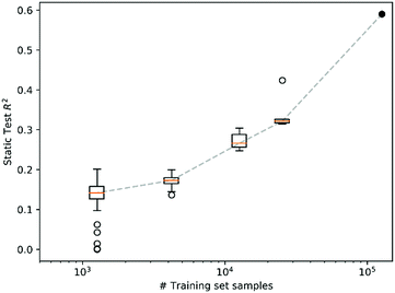
As noted above, a VAE was chosen as the basis for model 1 due to its latent space representation that enables prediction of other properties, such as the ASPM of model 2. This is a powerful approach for situations where the training set for the desired property is smaller than that of the related, less expensive property. The demonstration of this latent space exploitation to gain “expensive” information from “inexpensive” data motivated our use of the VAE instead of other algorithms that could also predict properties, such as band gap energy, from images. A regression model would be among the simplest algorithms for such a prediction but would not provide the compact latent space representation that we believe will become a key construct in the machine learning-based acceleration of materials science.To assess the size of materials data required for training the VAE and ASPM, we made subsets of the train set from the above models by randomly splitting it into 5 distinct sets, each with 20% of the train set size. Similarly, 10, 30 and 100 subsets were generated with 10%, 3.33% and 1% of the train set size, respectively. The VAE and ASPM (models 1 and 2) were trained from random initializations with each of these 145 subsets without use of the test set from models 1 and 2, enabling the evaluation of each trained model using a static test set (>5 104 materials), as summarized in Fig. 8. The R2 correlation increases dramatically with log test size, indicating that our successful training and use of VAE and cVAEs for experimental materials science was enabled by the >105 materials in the train set, and that expansion of the train set by additional order of magnitude would further improve the predictive power of the models.
Building more experimental materials databases of this size requires a revolution in data and metadata management. To date, computational materials datasets have been more amenable to machine learning due to relative ease in integration of data across research groups, whereas variations in experimental instruments and the lack of a framework to encode differences between instruments and experimental techniques limits assembly of large experimental databases. Consequently, the machine learning demonstrations in experimental solid state materials science, namely the work by Zakutayev et al.18 and the present work, utilize specific types of data acquired within a single research organization, and we believe these demonstrations lay the foundation for future generation of more broadly-applicable machine learning models3,36,37 in experimental solid state materials science so that the field may catch on the tremendous progress made in organic chemistry and drug discovery.19–23
Conclusion
Empowered by an unprecedented dataset of optical characterizations of metal oxide materials, we train a series of machine learning models employing convolutional and deep neural networks. A materials image autoencoder was developed by training a VAE using images of thin film materials acquired with a consumer flatbed scanner. The VAE, even though not trained with spectral information, encodes spectral characteristics in its information-rich latent space, enabling the development of a DNN model for predicting the full UV-vis absorption spectrum of a material from only its image. Band gap energies extracted from the predicted spectra match the uncertainty from the extraction algorithm and supersedes common ab initio methods for phase-pure materials. An additional model predicts the image of a hypothetical material based on its user-specified absorption pattern, providing the first example of a cVAE model trained exclusively of experimental materials data. This study has been enabled by the construction of a database of over 105 materials, demonstrating the utility of high throughput experiments with rigorous data management for further adoption of machine learning in experimental materials science.Methods
The dataset for this study was generated through a database search in the Materials Experiment and Analysis Database (MEAD) of the High-Throughput Experimentation (HTE) group at the Joint Center for Artificial Photosynthesis at Caltech. The dataset containing sample images, UV-vis spectra and composition can be found at 〈TBD〉. We cannot assert the absence of a bias towards either larger or smaller bandgap materials in this dataset since there is no comparably large dataset with optical properties on mixed metal oxides to compare. Samples were synthesized using ink-jet printing of precursors salts, typically metal nitrates, that are subsequently annealed to form metal oxides.31 Optical absorption spectra were recorded using an on-the-fly scanning UV-vis dual-sphere spectrometer as described elsewhere.22 Sample images were acquired using a commercially-available consumer flatbed scanner (EPSON Perfection V600) in reflection configuration as described elsewhere.23 The scanner acquired 1200 dpi images at a rate of 2.0 cm2 s−1, corresponding to 0.019 s per sample with our library design of approximately 1 mm2 samples on a square grid with 2 mm pitch. Original 2.1 mm × 2.1 mm sample images were 101 × 101 pixels with 24 bit color depth and were rescaled to 64 × 64 pixels via the python image library (pillow) with anti-aliasing.All calculations were performed on an Alienware Aurora R7 workstation equipped with an Intel i7-8700K@3.70 GHz CPU, 32 GB RAM, a Nvidia GTX1080Ti GPU with 12 GB dedicated GPU memory. Software used was Python version 3.6.4, Keras version 2.1.5, and TensorFlow version 1.1.0. The random test-train split was 30% test, 70% train. Since we base no decision on the test set an additional validation set is not generated. The test-train split is random.
Machine learning model descriptions
![[thin space (1/6-em)]](https://www.rsc.org/images/entities/char_2009.gif) 778 trainable parameters, less than one fifth the size of the training set. The output of the convolutional layers is flattened and passed to two layers μ and σ with 100 output dimensions (length of latent space embedding also optimized through hyperparameter optimization) and linear activation. The output of these was passed to a sampling layer z that samples the latent space via:
778 trainable parameters, less than one fifth the size of the training set. The output of the convolutional layers is flattened and passed to two layers μ and σ with 100 output dimensions (length of latent space embedding also optimized through hyperparameter optimization) and linear activation. The output of these was passed to a sampling layer z that samples the latent space via:| z = μ + aεeσ/2 |
![[thin space (1/6-em)]](https://www.rsc.org/images/entities/char_2009.gif) 288). The scaling of the binary cross entropy ensures convergence of both the KL-loss and the image reconstruction during training. When the reconstruction loss was not weighted the KL-loss converged but images were not reconstructed well.
288). The scaling of the binary cross entropy ensures convergence of both the KL-loss and the image reconstruction during training. When the reconstruction loss was not weighted the KL-loss converged but images were not reconstructed well.
An equivalent definition of L is the MSE loss scaled by the sum of the fractions of unexplained variance per energy. Interestingly the MSE between train and test set varies only slightly while the Re2 loss varies significantly.
Conflicts of interest
There are no conflicts to declare.Acknowledgements
This study is based upon work performed by the Joint Center for Artificial Photosynthesis, a DOE Energy Innovation Hub, supported through the Office of Science of the U.S. Department of Energy (Award No. DE-SC0004993).Notes and references
- R. Ramprasad, R. Batra, G. Pilania, A. Mannodi-Kanakkithodi and C. Kim, Machine learning in materials informatics: recent applications and prospects, npj Comput. Mater., 2017, 3, 54 CrossRef
.
- L. Ward and C. Wolverton, Atomistic calculations and materials informatics: A review, Curr. Opin. Solid State Mater. Sci., 2017, 21, 167–176 CrossRef CAS
.
-
S. K. Suram, M. Z. Pesenson and J. M. GregoireHigh Throughput Combinatorial Experimentation + Informatics = Combinatorial Science, in Information Science for Materials Discovery and Design 271–300, Springer International Publishing, 2015, DOI:10.1007/978-3-319-23871-5_14
.
- K. Rajan, Materials Informatics: The Materials “Gene” and Big Data, Annu. Rev. Mater. Res., 2015, 45, 153–169 CrossRef CAS
.
- R. Gómez-Bombarelli,
et al., Automatic Chemical Design Using a Data-Driven Continuous Representation of Molecules, ACS Cent. Sci., 2018, 4, 268–276 CrossRef PubMed
.
- Z. W. Ulissi, A. J. Medford, T. Bligaard and J. K. Nørskov, To address surface reaction network complexity using scaling relations machine learning and DFT calculations, Nat. Commun., 2017, 8, 14621 CrossRef PubMed
.
- C. Oses,
et al., Universal fragment descriptors for predicting properties of inorganic crystals, Nat. Commun., 2017, 8, 1–12 CrossRef PubMed
.
- O. Isayev,
et al., Materials Cartography: Representing and Mining Materials Space Using Structural and Electronic Fingerprints, Chem. Mater., 2015, 27, 735–743 CrossRef CAS
.
- K. T. Schütt,
et al., How to represent crystal structures for machine learning: Towards fast prediction of electronic properties, Phys. Rev. B: Condens. Matter Mater. Phys., 2014, 89, 1875 CrossRef
.
- J. Carrete, W. Li, N. Mingo, S. Wang and S. Curtarolo, Finding Unprecedentedly Low-Thermal-Conductivity Half-Heusler Semiconductors via High-Throughput Materials Modeling, Phys. Rev. X, 2014, 4, 18 Search PubMed
.
- R. Gómez-Bombarelli,
et al., Design of efficient molecular organic light-emitting diodes by a high-throughput virtual screening and experimental approach, Nat. Mater., 2016, 15, 1120–1127 CrossRef PubMed
.
- M. L. Green,
et al., Fulfilling the promise of the materials genome initiative with high-throughput experimental methodologies, Appl. Phys. Rev., 2017, 4, 011105 Search PubMed
.
- W. Setyawan and S. Curtarolo, High-throughput electronic band structure calculations: Challenges and tools, Comput. Mater. Sci., 2010, 49, 299–312 CrossRef
.
- F. Ren,
et al., Accelerated discovery of metallic glasses through iteration of machine learning and high-throughput experiments, Sci. Adv., 2018, 4, eaaq1566 CrossRef PubMed
.
- A. Ludwig, R. Zarnetta and S. Hamann, Development of multifunctional thin films using high-throughput experimentation methods, J. Mater. Chem. A, 2008, 99, 1144–1149 CAS
.
- M. Woodhouse and B. A. Parkinson, Combinatorial approaches for the identification and optimization of oxide semiconductors for efficient solar photoelectrolysis, Chem. Soc. Rev., 2008, 38, 197–210 RSC
.
- M. Woodhouse, G. S. Herman and B. A. Parkinson, Combinatorial Approach to Identification of Catalysts for the Photoelectrolysis of Water, Chem. Mater., 2005, 17, 4318–4324 CrossRef CAS
.
-
A. Zakutayev, et al., High Throughput Experimental Materials Database, 2017, DOI:10.7799/1407128
.
- H. Altae-Tran, B. Ramsundar, A. S. Pappu and V. Pande, Low Data Drug Discovery with One-Shot Learning, ACS Cent. Sci., 2017, 3, 283–293 CrossRef CAS PubMed
.
- V. Duros,
et al., Human versus Robots in the Discovery and Crystallization of Gigantic Polyoxometalates, Angew. Chem., Int. Ed., 2017, 56, 10815–10820 CrossRef CAS PubMed
.
- V. Dragone, V. Sans, A. B. Henson, J. M. Granda and L. Cronin, An autonomous organic reaction search engine for chemical reactivity, Nat. Commun., 2017, 8, 15733 CrossRef PubMed
.
-
L. M. Roch, et al., ChemOS: An Orchestration Software to Democratize Autonomous Discovery, 2018, DOI:10.26434/chemrxiv.5953606.v1
.
- C. Houben and A. A. Lapkin, Automatic discovery and optimization of chemical processes, Curr. Opin. Chem. Eng., 2015, 9, 1–7 CrossRef
.
- D. P. Kingma and M. Welling, Auto-encoding variational bayes, iclr 2016 stat.ml, 1312.6114v10 Search PubMed.
- A. Radford, L. Metz and S. Chintala, Unsupervised representation learning with deep convolutional generative adversarial networks, ICLR 2016 1511.06434v2 Search PubMed.
- E. O. Pyzer-Knapp, K. Li and A. Aspuru-Guzik, Learning from the Harvard Clean Energy Project: The Use of Neural Networks to Accelerate Materials Discovery, Adv. Funct. Mater., 2015, 25, 6495–6502 CrossRef CAS
.
- H. Döscher, J. F. Geisz, T. G. Deutsch and J. A. Turner, Sunlight absorption in water – efficiency and design implications for photoelectrochemical devices, Energy Environ. Sci., 2014, 7, 2951–2956 RSC
.
- S. Mitrovic,
et al., High-throughput on-the-fly scanning ultraviolet-visible dual-sphere spectrometer, Rev. Sci. Instrum., 2015, 86, 013904 CrossRef PubMed
.
- S. Mitrovic,
et al., Colorimetric Screening for High-Throughput Discovery of Light Absorbers, ACS Comb. Sci., 2015, 17, 176–181 CrossRef CAS PubMed
.
- Á. Morales-García, R. Valero and F. Illas, An Empirical, yet Practical Way To Predict the Band Gap in Solids by Using Density Functional Band Structure Calculations, J. Phys. Chem. C, 2017, 121, 18862–18866 CrossRef
.
- M. Schwarting, S. Siol, K. Talley, A. Zakutayev and C. Phillips, Automated algorithms for band gap analysis from optical absorption spectra, Materials Discovery, 2017, 10, 43–52 CrossRef
.
- G. Agranov, V. Berezin and R. H. Tsai, Crosstalk and microlens study in a color CMOS image sensor, IEEE Trans. Electron Devices, 2003, 50, 4–11 CrossRef
.
- L. van der Maaten, Accelerating t-SNE using Tree-Based Algorithms, J. Mach. Learn. Res., 2014, 15, 3221–3245 Search PubMed
.
- S. K. Suram, P. F. Newhouse and J. M. Gregoire, High Throughput Light Absorber Discovery, Part 1: An Algorithm for Automated Tauc Analysis, ACS Comb. Sci., 2016, 18, 673–681 CrossRef CAS PubMed
.
- H. Li,
et al., Preventing the coffee-ring effect and aggregate sedimentation by in situ gelation of monodisperse materials, Chem. Sci., 2018, 9, 7596–7605 RSC
.
- Y. Xue et al., Phase-Mapper: An AI Platform to Accelerate High Throughput Materials Discovery. aaai.org IAAI-17, pp. 4635–4642.
- H. S. Stein, S. Jiao and A. Ludwig, Expediting Combinatorial Data Set Analysis by Combining Human and Algorithmic Analysis, ACS Comb. Sci., 2017, 19, 1–8 CrossRef CAS PubMed
.
- B. Sanchez-Langeling and A. Aspuru-Guzik, Inverse molecular design using machine learning: Generative models for matter engineering, Science, 2018, 361(6400), 360–365 CrossRef PubMed
.
Footnote |
| † Electronic supplementary information (ESI) available: Details of model structure, additional model results, and file containing all model weights. See DOI: 10.1039/c8sc03077d; The full dataset can be found at DOI: 10.22002/D1.1103 |
| This journal is © The Royal Society of Chemistry 2019 |

