Machine-learning-guided identification of protein secondary structures using spectral and structural descriptors

Abstract

Interrogation of the secondary structures of proteins is essential for designing and engineering more effective and safer protein-based biomaterials and other classes of theranostic materials. Protein secondary structures are commonly assessed using circular dichroism spectroscopy, followed by relevant downstream analysis using specialized software. As many proteins have complex secondary structures beyond the typical α-helix and β-sheet configurations, and the derived secondary structural contents are significantly influenced by the selection of software, estimations acquired through conventional methods may be less reliable. Herein, we propose the implementation of a machine-learning-based approach to improve the accuracy and reliability of the classification of protein secondary structures. Specifically, we leverage supervised machine learning to analyze the circular dichroism spectra and relevant attributes of 112 proteins to predict their secondary structures. Based on a range of spectral, structural, and molecular features, we systematically evaluate the predictive performance of numerous supervised classifiers and identify optimal combinations of algorithms with descriptors to achieve highly accurate and precise estimations of protein secondary structures. We anticipate that this work will offer a deeper insight into the development of machine-learning-based approaches to streamline the delineation of protein structures for different biological and biomedical applications.

---

1. Introduction

Understanding the structures of proteins is crucial for designing and engineering effective and safe biomaterials for disease theranostic and nanomedicine applications.^1–5 Many of these bioapplications rely on specific interactions between biomaterials and proteins to induce the intended diagnostic and therapeutic effects. For example, the adsorption of certain target proteins on pristine and functionalized biomaterial surfaces and their subsequent interactions have been widely exploited for the detection of diseases, including cancer, infectious diseases, and neurodegenerative diseases.^6–11 To achieve the anticipated theranostic effects, biomaterials are typically engineered to either enhance or disrupt the functionalities of the target proteins, which may be realized by modulating their conformational and structural stability.^12–15 As such, comprehensive characterization and understanding of protein structures are essential for gaining a deeper insight into biomaterial–protein interactions and the elicited biological impacts.

Over the years, many microscopic and spectroscopic technqiues have been employed to better understand protein structures. For example, cryo electron microscopy is actively being utilized to resolve the three-dimensional (3D) structures of proteins at near-atomic resolution.^16,17 Fluorescence spectroscopy is commonly used to examine the tertiary structure of proteins,^18,19 while their secondary structure is widely characterized using near- and far-ultraviolet (UV) circular dichroism (CD) spectroscopy.^20,21 The secondary structure of a protein is the local spatial conformation of its polypeptide backbone, and can be employed to predict the overall 3D structure of a protein. In general, the secondary structure of a protein can be broadly classified into two predominant types, i.e., alpha helix (α-helix) and beta sheet (β-sheet) structures. The α-helix structure is a right-handed spiral structure within a single polypeptide chain, while the β-sheet structure comprises at least two adjacent stretches of polypeptide chain in a fully extended conformation. It is, nevertheless, noteworthy that other less common types of secondary structure exist too. These include beta turn (β-turn) or beta bend (β-bend) and omega loop, which are non-regular and non-repeating secondary structural motifs. Also, while a protein may assume a predominant secondary structure, the same protein may have certain percentages of other configurations as well. For instance, although the secondary structure of human serum albumin is predominantly α-helix, which accounts for 67%, this protein has 10% turns and 23% random coils.²² The presence of the different secondary structural components is essential for regulating the activities and functionalities of proteins, including protein folding and protein–ligand interactions.

One of the most common techniques to elucidate protein secondary structure is CD spectroscopy.^23–25 In partic, this optical spectroscopic technique relies on the difference in the absorption of the right- and left-circularly polarized light by a protein to infer its secondary structure. Due to the distinct arrangement of the polypeptide chains of α-helix and β-sheet structures, the CD spectra of these structures are unique. However, as many proteins have complex or less common secondary structures, it is not always possible to identify these structures directly from the obtained CD spectra. To derive the different constituents of the secondary structure of a particular protein, the acquired protein CD spectrum is typically analyzed with specialized software leveraging distinct algorithms, such as K2D2, K2D3, and BeStSel.^21,26,27 For instance K2D2 uses a self-organizing map algorithm, which is a form of neural network, to derive the secondary structure maps of proteins and estimate the content of α-helix and β-strand. K2D3, which is an improvement of K2D2, capitalizes on a k-nearest neighbors algorithm to predict protein secondary structures. It is, nonetheless, important to note that the estimated secondary structural components are heavily influenced by the selection of the software, which may render the eventual estimations less reliable.

In recent years, there have been active explorations into the development and applications of machine learning to streamline the design and engineering of biomaterials.^28–35 Specifically, numerous machine-learning-based techniques have been developed to uncover previously unknown biomaterials as well as to predict their physicochemical properties, particularly from their optical spectra.^36–39 For example, in a recent study, a one-dimensional (1D) convolutional neural network was implemented to distinguish between different organic compounds based on their near-infrared spectra.⁴⁰ In a separate work, a supervised random forest classifier was used to identify organic compounds from their visible light spectra.⁴¹ With its capability to recognize subtle spectral attributes and estimate the compositions and structures of samples from their optical spectra, machine learning has emerged as a promising tool to examine a wide range of spectral data, including CD spectra.

In this study, we sought to leverage supervised machine learning to analyze the far-UV (190–260 nm) CD spectra of 112 proteins and identify their predominant secondary structures. We systematically assessed the predictive performance of several supervised classifiers using numerous spectral, structural, and molecular features. Ultimately, we demonstrated optimal combinations of supervised learning algorithms and descriptors to realize reliable and computationally cost-effective predictions of protein secondary structures.

2. Results and discussion

To start with, capitalizing on the Protein Circular Dichroism Data Bank (PCDDB),⁴² we curated a dataset comprising 112 proteins with their molecular properties (i.e., molecular weight, number of residues, and mean residue weight), far-UV CD spectra, and secondary structural contents (i.e., α-helix, β-strand, loop, bend, and bonded turn) (ESI Excel File 1†). According to the characteristic spectral shape and secondary structural contents, we grouped the proteins into three unique classes, i.e., proteins with α-helix, β-sheet, and other secondary structures (Fig. 1). We then quantitatively analyzed the spectral, structural, and molecular characteristics of these proteins.

Fig. 1 Secondary structural and molecular properties of proteins. (a) Representative circular dichroism (CD) spectra of proteins with two distinct secondary structures (i.e., primarily α-helix and β-sheet structures). (b–f) Proportions of (b) α-helix, (c) β strands, (d) loop, (e) bend, and (f) bonded turn of the three classes of proteins. (g–i) Distributions of (g) molecular weight, (h) number of residues, and (i) mean residue weight of the three classes of proteins. n = 31 for proteins with predominantly α-helix secondary structure, 38 for proteins with predominantly β-sheet secondary structure, and 43 for proteins having predominantly a mixture of α-helix and β-sheet secondary structures. * p < 0.05, *** p < 0.001, and **** p < 0.0001 based on the nonparametric Kruskal–Wallis test.

Proteins with primarily α-helical structure typically have two negative peaks at about 208 and 222 nm as well as a positive peak at about 190 nm in their far-UV CD spectra (Fig. 1a). In contrast, the CD spectra of proteins with a predominantly β-sheet structure have a negative peak at around 210–220 nm and a positive peak at approximately 195–205 nm. Proteins with other secondary structures, such as those with less common secondary structures or those with a mixture of α-helical and β-sheet structures, displayed more complex CD spectra with less identifiable unique spectral features. We next examined the secondary structural contents of the three classes of proteins (Fig. 1b–f). As anticipated, the α-helical proteins had the highest content of α-helix (Fig. 1b), but the lowest content of β-strand (Fig. 1c), as compared to the other two classes of proteins. In contrast, the α-helix and β-strand contents of the β-sheet proteins were the lowest and highest, respectively, among the three protein classes. A deeper analysis of other secondary structural components of the proteins revealed that the α-helical proteins had the lowest loop and bend contents (Fig. 1d and e), while those of proteins with β-sheet and other secondary structures were not statistically significantly different. Next, we sought to assess the molecular properties of the three classes of proteins, particularly their molecular weight, number of residues, and mean residue weight. Intriguingly, we noted that these proteins had comparable molecular weight, number of residues, and mean residue weight (Fig. 1g–i), suggesting that there may not be a direct correlation between these molecular properties and the secondary structure of proteins.

After statistically assessing the structural and molecular features of all proteins, we sought to evaluate if supervised learning algorithms could be employed to predict the secondary structures of these proteins. Seven distinct algorithms were selected, notably logistic regression, random forest, gradient boosting, extreme gradient boosting, k-nearest neighbors, support vector machine, and neural network. For all supervised learning analysis, the datasets were randomly split into 75% training and 25% testing sets, which were used for classifier training and testing, respectively.

To begin with, we were motivated to examine the predictive capacity of the algorithms based on various protein structural and molecular features (Fig. 2). Here, all datasets comprised eight features, i.e., molecular weight, number of residues, mean residue weight, α-helix, β-strand, loop, bend, and bonded turn contents, which collectively served as the inputs to the classifiers, while the predicted protein classes were the target outputs. To ascertain if particular features had a higher correlation with the target protein classes, we quantitatively scored and ranked the eight structural and molecular features (Fig. 2a). Based on information gain ratio, which is one of the common metrics used to analyze variable importance, β-strand and α-helix contents emerged as the two highest ranked attributes. In fact, with gain ratios of 0.516 and 0.492, respectively, which were significantly much higher than those of the other features, β-strand and α-helix contents were highly discriminatory, which could be capitalized on to delineate protein classes effectively. Analysis of the distribution of all proteins in a two-dimensional (2D) space using t-distributed stochastic neighbor embedding (t-SNE) revealed that the three protein classes were well separated with negligible overlapping (Fig. 2b). Leveraging the training dataset, we proceeded to tune the different hyperparameters of all supervised learning algorithms to produce the highest classification metrics (ESI Fig. S1†). We observed that, except for k-nearest neighbors, the other six algorithms had outstanding predictive capacity, where all values of area under the curve (AUC) were above 0.96. Specifically, gradient boosting, extreme gradient boosting, and random forest had AUCs of more than 0.98 and classification accuracy, F1 values, precision, and recall of at least 0.94. A closer examination of the classification performance of the best performing algorithm, i.e., gradient boosting, unveiled that all 24 α-helical proteins, 28 β-sheet proteins (out of a possible 29), and 27 proteins with other secondary structures (out of a possible 31) were correctly classified. Based on the optimized algorithm hyperparameters and testing dataset, we then assessed the algorithm classification metrics, and noted that gradient boosting, random forest, and extreme gradient boosting were the best performing classifiers (Fig. 2c). This corroborated our observation during classifier training. The three algorithms showed perfect AUCs of 1.000. In fact, as the best performing classifier, gradient boosting predicted all protein classes correctly, which was reflected in the values of its accuracy, precision, recall, and F1 score, as well as its confusion matrix (Fig. 2d). It is important to highlight that, as compared to their predictive performance against the training dataset, most of the algorithms showed much improved classification capacity against the testing dataset.

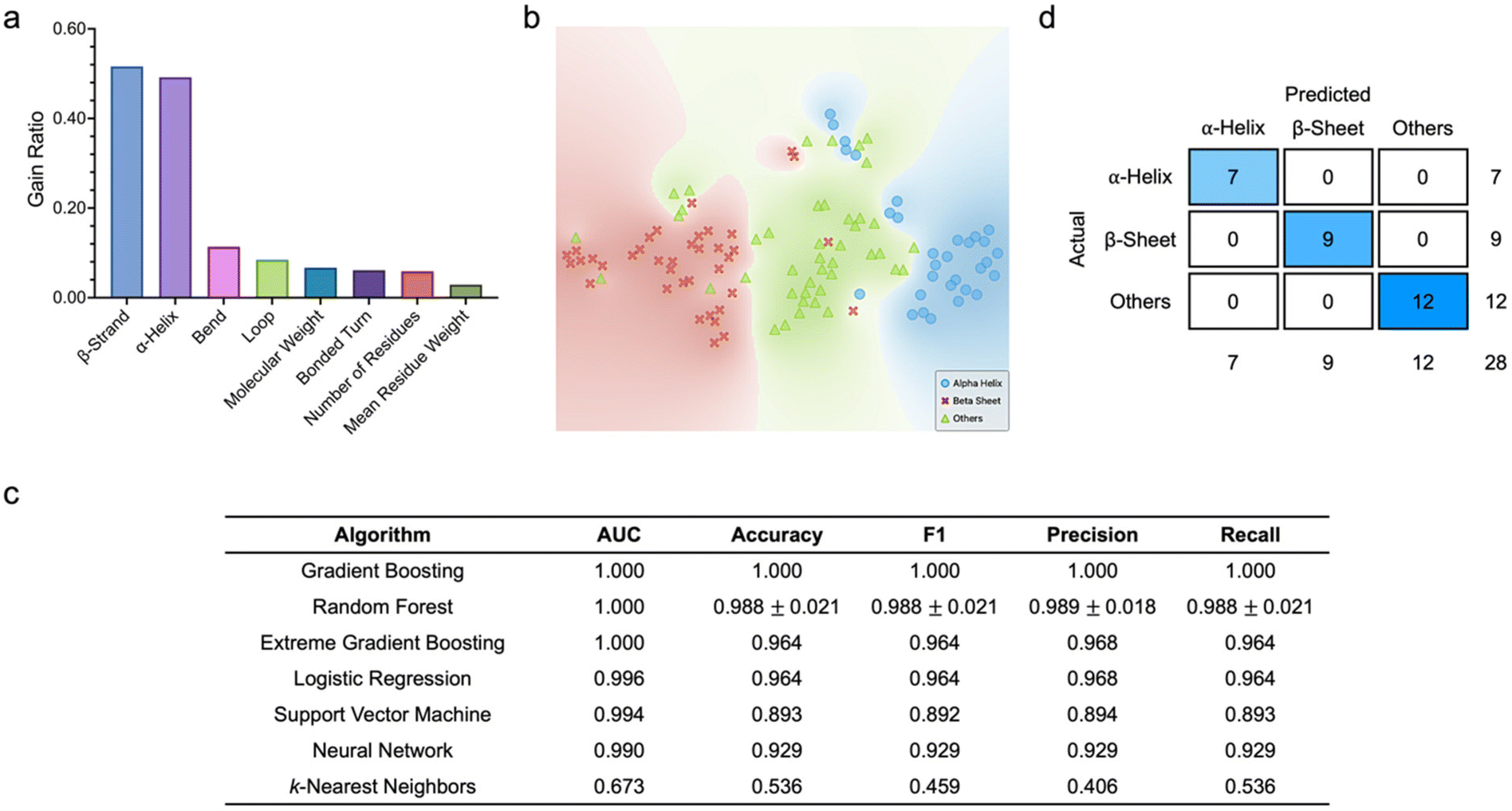Fig. 2 Classification of protein secondary structures based on structural and molecular descriptors. (a) Feature scoring and ranking based on information gain ratio. (b) t-SNE plot showing the 2D distribution of the three classes of proteins. (c) Comparison of the testing performance of all supervised machine learning algorithms leveraging structural and molecular features. Data is represented as mean ± standard deviation. n = 3. (d) Confusion matrix of the best performing classifier (i.e., gradient boosting).

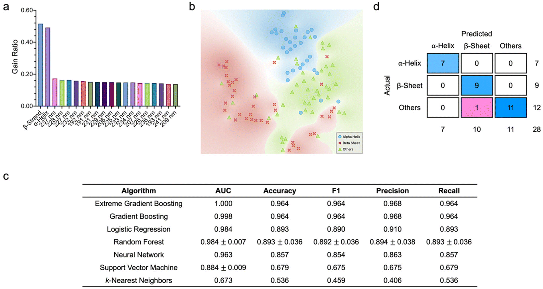
Next, we aimed to assess if similar excellent predictive performance demonstrated by most of the supervised learning algorithms could be maintained if the structural and molecular features were replaced with spectral features (Fig. 3). Here, the far-UV CD spectra of all proteins from 190 nm to 260 nm were employed. With a step size of 1 nm, both the training and testing datasets comprised 71 features, where each feature corresponded to specific wavelength. Quantitative scoring of all spectral features based on information gain ratio did not reveal features with especially high discriminatory power (Fig. 3a). However, we still noted that spectral attributes at wavelengths between 225 and 237 nm, 206 and 209 nm, as well as 191 and 193 nm ranked highly as variables with higher correlation with the target protein classes, while those at wavelengths from 250 to 260 nm appeared to have no correlation. Through t-SNE, we observed the distinct 2D distribution of the three protein classes (Fig. 3b). Based on the tuned algorithm hyperparameters using the training dataset, gradient boosting emerged as the best performing classifier with an AUC of 0.853, an accuracy of 0.690, and a precision of 0.703 (ESI Fig. S2†). This classifier correctly predicted 19 α-helical proteins (out of a possible 24), 19 β-sheet proteins (out of a possible 29), and 20 proteins with other secondary structures (out of a possible 31). Support vector machine and neural network were the next best performing classifiers with AUCs of at least 0.83 and accuracy and precision values above 0.660. As opposed to those obtained based on structural and molecular features, all quantitative metrics of most of the classifiers acquired using spectral features decreased substantially. This trend was also reflected in the classification performance of all algorithms against the testing dataset (Fig. 3c). Assessment of the confusion matrix of gradient boosting, which was the best performing classifier, unveiled that five α-helical proteins (out of a possible seven), five β-sheet proteins (out of a possible nine), and eight proteins with other secondary structures (out of a possible 12) were correctly classified (Fig. 3d).

Fig. 3 Classification of protein secondary structures based on full spectral descriptors. (a) Feature scoring and ranking based on information gain ratio. Only the first 20 features are displayed. (b) t-SNE plot showing the 2D distribution of the three classes of proteins. (c) Comparison of the testing performance of all supervised machine learning algorithms leveraging full spectral data. Data is represented as mean ± standard deviation. n = 3. (d) Confusion matrix of the best performing classifier (i.e., gradient boosting).

Although the secondary structures of proteins are typically inferred through their CD spectra, it is noteworthy that not all spectral information is useful for estimating the secondary structural contents. For instance, the α-helical structure of proteins can be identified from their CD spectra based on only the two negative peaks at approximately 208 and 222 nm and a positive peak at around 190 nm. This suggests that the spectral components at other wavelengths have less contribution toward the delineation of this class of proteins. Additionally, depending on the experimental parameters and conditions (e.g., spectral acquisition step size, quality of instruments, and so on), the acquired CD spectra may contain interfering signals. Therefore, all these factors may collectively explain the relatively lower values of the quantitative metrics of all supervised classifiers when the full spectral descriptors were employed in place of the structural and molecular descriptors.

Next, as an indirect comparison, we were motivated to assess the performance of some of the commonly used platforms in predicting protein secondary structures. To this end, we sought to infer the secondary structures of several proteins by estimating their structural contents using K2D2 and K2D3 (ESI Excel File 2†). Since both platforms can only estimate the percentages of α-helix and β-sheet from CD spectra, we specifically selected proteins with predominantly those two secondary structures from the testing dataset for evaluations. Intriguingly, we noted that the estimated secondary structural contents were far from satisfactory. For instance, for all seven α-helical proteins, the calculated percentages of α-helix were substantially lower than those of β-sheet, suggesting that the platforms classified these proteins as those with predominantly β-sheet configuration. For the nine β-sheet proteins, despite the considerably higher calculated percentages of β-sheet than those of α-helix, we observed a low fidelity between the predicted and input CD spectra. It is also worth highlighting that, since the CD spectrum can only be analyzed one at a time, the process is time-consuming, especially when dealing with a large number of spectra.

To further understand the classifier predictive ability, we next sought to assess how the classification metrics of all supervised learning algorithms would be influenced by adding structural and molecular descriptors to the full spectral features (Fig. 4). Here, both the training and testing datasets had 79 features. As anticipated, β-strand and α-helix contents, followed by the spectral features at 225–237 nm, 206–209 nm, and 191–193 nm were the most highly ranked variables (Fig. 4a). Like in our previous observations, the three classes of proteins were distinctly separated with minimal overlapping in a 2D space (Fig. 4b). Leveraging the optimized algorithm hyperparameters and the training dataset, we noted that extreme gradient boosting emerged as the best performing algorithm with an AUC of 0.980 and classification accuracy, F1 score, precision, and recall of around 0.952 (ESI Fig. S3†). Gradient boosting and random forest were the next best performing algorithms with AUCs of 0.975 and 0.945 ± 0.005, respectively. In contrast, the k-nearest neighbors algorithm was the worst performing algorithm with an AUC of 0.589. Analysis of the confusion matrix of extreme gradient boosting elucidated that this algorithm correctly classified all α-helical proteins, 28 β-sheet proteins (out of a possible 29), and 28 proteins with other secondary structures (out of a possible 31). Based on the tuned hyperparameters, we then characterized the algorithm predictive capacity using the testing dataset. Similarly, extreme gradient boosting and gradient boosting showed the highest classification metrics with AUCs of at least 0.998 and accuracy, F1 values, precision, and recall of at least 0.964 (Fig. 4c). Meanwhile, k-nearest neighbors was again the worst performing algorithm. Analysis of the confusion matrix of extreme gradient boosting revealed that this algorithm correctly classified all α-helical and β-sheet proteins and missed only one protein with other secondary structures (Fig. 4d).

Fig. 4 Classification of protein secondary structures based on full spectral, structural, and molecular descriptors. (a) Feature scoring and ranking based on information gain ratio. Only the first 20 features are displayed. (b) t-SNE plot showing the 2D distribution of the three classes of proteins. (c) Comparison of the testing performance of all supervised machine learning algorithms leveraging full spectra as well as structural and molecular features. Data is represented as mean ± standard deviation. n = 3. (d) Confusion matrix of the best performing classifier (i.e., extreme gradient boosting).

It is intriguing to note that the introduction of the eight structural and molecular descriptors significantly improved the quantitative metrics of most supervised classifiers. For instance, against the testing datasets, the AUCs of extreme gradient boosting, gradient boosting, and logistic regression increased from 0.724, 0.837, and 0.790, respectively, to higher than 0.980 (Fig. 3c and 4c). In fact, all quantitative metrics of the seven classifiers were enhanced considerably, except for the precision of k-nearest neighbors. Against the training datasets, however, all the quantitative metrics of k-nearest neighbors decreased substantially, while a reverse trend was noted from those of the other six classifiers (ESI Fig. S2 and S3†).

As highlighted previously, the secondary structures of proteins are commonly estimated from their characteristic CD spectra. While the full CD spectra with many spectral attributes contain a huge amount of information, some of the information are redundant and not all are essential for delineating protein secondary structures. Moreover, some of the full CD spectra may contain noise, which may be introduced during the spectral acquisition process. This may then complicate the characterization of protein structures. As such, it is important to extract only the most discriminatory features from the full CD spectra to improve the quality and reliability of protein secondary structure identification.

To this end, in this part of our study, we sought to transform the high-dimensional full spectral datasets into their low-dimensional counterparts and assess the classification performance of all classifiers against these newly generated datasets (Fig. 5). To start with, through principal component analysis (PCA), we reduced the dimensionality of all CD spectra from 71 wavelength components to six principal components. The number of principal components was especially selected to account for more than 90% of spectral data variance (ESI Fig. S4†). With gain ratios of 0.135, 0.102, and 0.099, the first, fifth, and second principal components, i.e., PC1, PC5, and PC2, respectively, were the most important features (Fig. 5a). Although PC2 ranked lower than PC5 in terms of gain ratio, it is noteworthy that PC2 captured about 26% of spectral data variance while PC5 accounted for only about 5%. As such, capitalizing on only PC1 and PC2 to create a score plot, we visualized the 2D distribution of the three protein classes, where a high degree of separation with some overlapping was noted (Fig. 5b). Further interrogation of protein distributions using PC1 and PC2 showed the highly distinct separation of α-helical and β-sheet proteins (Fig. 5c). Nonetheless, the distributions of proteins with other secondary structures overlapped to a certain degree with those of the other two protein classes. Assessment of the loading spectra of both PC1 and PC2 revealed unique trends in the contributions of each spectral attribute to the two principal components (Fig. 5d).

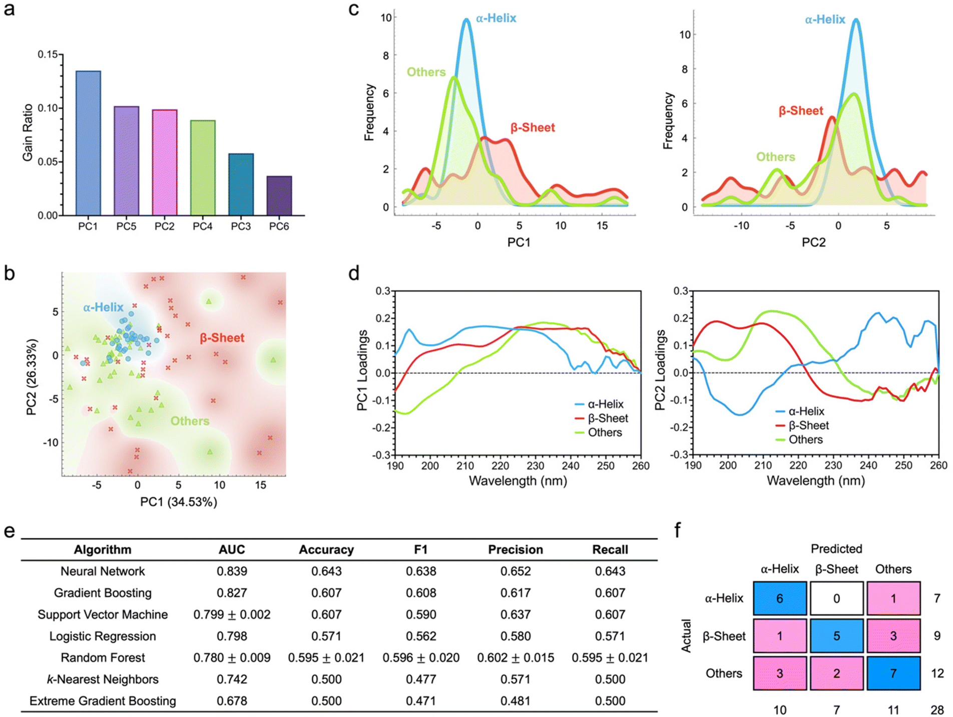Fig. 5 Classification of protein secondary structures based on dimensionally reduced spectral descriptors. (a) Feature scoring and ranking based on information gain ratio. (b) Score plot showing the 2D distribution of the three classes of proteins. (c) The corresponding histogram representations of PC1 and PC2 of individual proteins. (d) Loading spectra of PC1 and PC2. (e) Comparison of the testing performance of all supervised machine learning algorithms leveraging dimensionally reduced spectral data. Data is represented as mean ± standard deviation. n = 3. (f) Confusion matrix of the best performing classifier (i.e., neural network).

Adopting a similar approach, we then employed the training dataset to optimize various algorithm hyperparameters and evaluated the generated classification parameters (ESI Fig. S5†). All trained classifiers showed good predictive capacity. Of all algorithms, support vector machine demonstrated the highest quantitative metrics with an AUC of 0.841 and an accuracy and a precision of close to 0.7. This classifier managed to correctly classify 18 α-helical proteins (out of a possible 24), 19 β-sheet proteins (out of a possible 29), and 19 proteins with other secondary structures (out of a possible 31). As the next best performing classifiers, extreme gradient boosting, random forest, and gradient boosting had AUCs of above 0.83, although random forest had much higher mean values of accuracy, F1 score, precision, and recall. Against the testing dataset, neural network showed the highest AUC of 0.839 (Fig. 5e). With this classifier, six α-helical proteins (out of a possible seven), five β-sheet proteins (out of a possible nine), and seven proteins with other secondary structures (out of a possible 12) could be correctly predicted (Fig. 5f). Gradient boosting and support vector machine had the next highest AUCs of 0.827 and 0.799 ± 0.002, respectively.

Interestingly, examining the classifier performance on the training datasets as the full spectral descriptors were switched to their dimensionally reduced counterparts, we noted that, both neural network and logistic regression showed substantially improved accuracy, F1 values, precision, and recall (ESI Fig. S2 and S5†). This trend became increasingly more apparent when analyzing the classifier performance against the testing datasets (Fig. 3 and 5). In fact, three of the evaluated classifiers, i.e., neural network, logistic regression, and k-nearest neighbors, had enhanced AUC, accuracy, precision, recall, and F1 values. Support vector machine, while having the same accuracy and recall values, also had improved AUC and precision with the use of dimensionally reduced spectral data.

It is crucial to highlight that the analysis of full spectral data using machine learning may require significant computational resources and processing time, especially if the datasets consist of a huge number of entries and spectral features. The high dimensionality of these datasets may render classifier training and generalization challenging. Furthermore, for certain algorithms with numerous tunable hyperparameters like neural network, computational effort and processing time increase substantially along with an increase in certain hyperparameter values (e.g., number of neurons in hidden layers). The use of dimensionality reduction methods, such as PCA, can address some of the highlighted issues to a certain extent. As illustrated in this study, most of the important spectral information (more than 90% of data variance) could still be captured with the use of only six principal components, as opposed to the full 71 spectral features. The more than 10-fold reduction in the dataset dimensionality significantly reduced the computational effort and analysis time of all classifiers. In addition, the predictive capacity of some classifiers could be augmented considerably with the use of dimensionally reduced datasets. All these collectively demonstrate the advantages of coupling dimensionality reduction techniques with supervised machine learning to enhance the prediction of protein secondary structures.

3. Conclusion

Herein, we employed a machine-learning-based approach to augment the prediction of the secondary structures of 112 proteins through their spectral, structural, and molecular descriptors. The predictive capacity of various supervised classifiers was systematically assessed and optimal combinations of machine learning algorithms with descriptors were identified to realize more accurate and precise estimations of protein secondary structures. Importantly, we showed the merit of coupling a dimensionality reduction technique with supervised learning and that the use of dimensionally reduced datasets could improve certain classification metrics of some classifiers. This approach is especially beneficial when dealing with datasets comprising a large number of samples and spectral features (e.g., hundreds to thousands of features) and when other descriptors, such as estimated α-helix and β-strand contents, are not readily available. Since the spectral dataset used in our work comprises well characterized proteins, the demonstrated machine-learning-assisted strategy can be readily extended to investigate the secondary structures of unknown biomolecules. Furthermore, as CD spectra are 1D spectra, it may be possible to adopt our approach to analyze other types of 1D spectra, notably fluorescence, Raman, and infrared spectra, to further understand the structures of different biomolecules. Overall, we anticipate that this study will provide a deeper insight into the use of machine learning for the analysis of protein structures to enhance the engineering of protein-based biomaterials and other types of theranostic materials for biological and biomedical applications.

4. Methods

Spectral dataset acquisition and pre-processing

The CD spectral dataset with the associated protein structural and molecular information were obtained from the Protein Circular Dichroism Data Bank (PCDDB).⁴² Incomplete and duplicate data were removed, yielding a total of 112 protein entries (ESI Excel File 1†). All CD spectra were normalized and corrected for baseline prior to further processing.

Feature scoring, t-distributed stochastic neighbor embedding (t-SNE) analysis, and principal component analysis (PCA)

Feature scoring, t-SNE, and PCA were performed using Orange Data Mining (University of Ljubljana, Slovenia). For feature scoring, information gain ratio was selected as the assessment metric. For t-SNE analysis, spectral initialization and Euclidean distance metric were chosen, and perplexity was set to 10. For PCA, the number of principal components was selected to account for more than 90% of data variance.

Supervised machine learning analysis

The supervised machine learning evaluations were performed using Orange Data Mining (University of Ljubljana, Slovenia). The dataset was split into 75% training set and 25% testing set randomly to minimize selection bias. Seven supervised machine learning algorithms, i.e., logistic regression, random forest, gradient boosting, extreme gradient boosting, k-nearest neighbors, support vector machine, and neural network, were implemented and their classification performance was evaluated according to five quantitative metrics, i.e., area under the curve (AUC), accuracy, F1 score, precision, and recall. During classifier training, based on a stratified 10-fold cross validation, the hyperparameters of all algorithms (i.e., (1) logistic regression: regularization type and strength, (2) random forest: number of trees, (3) gradient boosting and (4) extreme gradient boosting: number of trees, learning rate, regularization, and limit depth of individual trees, (5) k-nearest neighbors: number of neighbors, metric, and weight, (6) support vector machine: cost, regression loss epsilon, kernel, and iteration limit, and (7) neural network: number of neurons in hidden layers, activation function, solver, regularization, and maximum number of iterations (ESI Table S1†) were tuned using the training datasets to yield the highest classification metrics. These optimized hyperparameters (ESI Tables S2 to S5†) were then used to evaluate the testing performance of the classifiers.

Statistical analysis

All quantitative data were statistically examined using GraphPad Prism 10.3 (GraphPad Software Inc., USA). Data distribution was first assessed using the Shapiro–Wilk test for normality. Nonparametric data was evaluated using the Kruskal–Wallis test coupled with Dunn's multiple comparisons test. Statistically significant differences were accepted for * p < 0.05, *** p < 0.001, and **** p < 0.0001.

Author contributions

K. conceived and designed the study. K. preprocessed and curated the protein dataset. K. performed feature scoring, t-SNE, PCA, and statistical analysis. Z.W. conducted supervised learning analysis. All authors wrote, read, revised, and approved the submission of the manuscript.

Data availability

The data supporting this article have been included as part of the ESI.†

Conflicts of interest

There are no conflicts of interest to declare.

Acknowledgements

The authors would like to acknowledge the departmental start-up fund of Kenry from the Department of Pharmacology and Toxicology, R. Ken Coit College of Pharmacy, University of Arizona.

References

1. A. Miserez, J. Yu and P. Mohammadi, Chem. Rev., 2023, 123, 2049–2111.
2. R. Gharios, R. M. Francis and C. A. DeForest, Matter, 2023, 6, 4195–4244.
3. A. Solomonov, A. Kozell and U. Shimanovich, Angew. Chem., Int. Ed., 2024, 63, e202318365.
4. B. Çalbaş, A. N. Keobounnam, C. Korban, A. J. Doratan, T. Jean, A. Y. Sharma and T. A. Wright, Biomater. Sci., 2024, 12, 2841–2864.
5. Kenry, Nanoscale, 2024, 16, 7874–7883.
6. S. O. Kelley, C. A. Mirkin, D. R. Walt, R. F. Ismagilov, M. Toner and E. H. Sargent, Nat. Nanotechnol., 2014, 9, 969–980.
7. Kenry, A. Geldert, X. Zhang, H. Zhang and C. T. Lim, ACS Sens., 2016, 1, 1315–1321.
8. Kenry, A. Geldert, Z. Lai, Y. Huang, P. Yu, C. Tan, Z. Liu, H. Zhang and C. T. Lim, Small, 2017, 13, 1601925.
9. A. Geldert, Kenry, X. Zhang, H. Zhang and C. T. Lim, Analyst, 2017, 142, 2570–2577.
10. A. Geldert, Kenry and C. T. Lim, Sci. Rep., 2017, 7, 17510.
11. S. Miyamura, R. Oe, T. Nakahara, H. Koresawa, S. Okada, S. Taue, Y. Tokizane, T. Minamikawa, T.-A. Yano, K. Otsuka, A. Sakane, T. Sasaki, K. Yasutomo, T. Kajisa and T. Yasui, Sci. Rep., 2023, 13, 14541.
12. W. C. Lee, C. H. Y. X. Lim, H. Shi, L. A. L. Tang, Y. Wang, C. T. Lim and K. P. Loh, ACS Nano, 2011, 5, 7334–7341.
13. W. C. Lee, C. H. Lim, Kenry, C. Su, K. P. Loh and C. T. Lim, Small, 2015, 11, 963–969.
14. J. Dembélé, J.-H. Liao, T.-P. Liu and Y.-P. Chen, ACS Appl. Mater. Interfaces, 2023, 15, 432–451.
15. A. Gorantla, J. T. V. E. Hall, A. Troidle and J. M. Janjic, Micromachines, 2024, 15, 533.
16. K. M. Yip, N. Fischer, E. Paknia, A. Chari and H. Stark, Nature, 2020, 587, 157–161.
17. R. Castells-Graells, K. Meador, M. A. Arbing, M. R. Sawaya, M. Gee, D. Cascio, E. Gleave, J. É. Debreczeni, J. Breed, K. Leopold, A. Patel, D. Jahagirdar, B. Lyons, S. Subramaniam, C. Phillips and T. O. Yeates, Proc. Natl. Acad. Sci. U. S. A., 2023, 120, e2305494120.
18. V. K. Sharma and D. S. Kalonia, J. Pharm. Sci., 2003, 92, 890–899.
19. Y. Saricay, B. J. de Kort, H. Yigit-Gercek and E. H. C. Dirksen, Anal. Biochem., 2021, 630, 114331.
20. N. J. Greenfield, Nat. Protoc., 2006, 1, 2876–2890.
21. A. Micsonai, F. Wien, L. Kernya, Y.-H. Lee, Y. Goto, M. Réfrégiers and J. Kardos, Proc. Natl. Acad. Sci. U. S. A., 2015, 112, E3095–E3103.
22. V. Mishra and R. J. Heath, Int. J. Mol. Sci., 2021, 22, 8411.
23. Kenry, K. P. Loh and C. T. Lim, Small, 2015, 11, 5105–5117.
24. Kenry, K. P. Loh and C. T. Lim, Nanoscale, 2016, 8, 9425–9441.
25. Kenry, T. Yeo, P. N. Manghnani, E. Middha, Y. Pan, H. Chen, C. T. Lim and B. Liu, ACS Nano, 2020, 14, 4509–4522.
26. C. Perez-Iratxeta and M. A. Andrade-Navarro, BMC Struct. Biol., 2008, 8, 25.
27. C. Louis-Jeune, M. A. Andrade-Navarro and C. Perez-Iratxeta, Proteins: Struct., Funct., Bioinf., 2012, 80, 374–381.
28. J. Kerner, A. Dogan and H. von Recum, Acta Biomater., 2021, 130, 54–65.
29. A. Suwardi, F. Wang, K. Xue, M.-Y. Han, P. Teo, P. Wang, S. Wang, Y. Liu, E. Ye, Z. Li and X. J. Loh, Adv. Mater., 2022, 34, 2102703.
30. S. M. McDonald, E. K. Augustine, Q. Lanners, C. Rudin, L. Catherine Brinson and M. L. Becker, Nat. Commun., 2023, 14, 4838.
31. Kenry, Adv. Theory Simul., 2023, 6, 2300122.
32. S. Dhoble, T.-H. Wu and Kenry, Angew. Chem., Int. Ed., 2024, 63, e202318380.
33. C. Sahli and Kenry, ACS Mater. Lett., 2024, 6, 4697–4709.
34. Kenry, Nanoscale, 2024, 16, 19656–19668.
35. S. You, Y. Fan, Y. Chen, X. Jiang, W. Liu, X. Zhou, J. Zhang, J. Zheng, H. Yang and X. Hou, Cell Rep. Phys. Sci., 2024, 5, 102116.
36. H. S. Stein, D. Guevarra, P. F. Newhouse, E. Soedarmadji and J. M. Gregoire, Chem. Sci., 2019, 10, 47–55.
37. L. Simine, T. C. Allen and P. J. Rossky, Proc. Natl. Acad. Sci. U. S. A., 2020, 117, 13945–13948.
38. J. F. Joung, M. Han, J. Hwang, M. Jeong, D. H. Choi and S. Park, JACS Au, 2021, 1, 427–438.
39. N. T. Hung, R. Okabe, A. Chotrattanapituk and M. Li, Adv. Mater., 2024, 36, 2409175.
40. X. Chen, Q. Chai, N. Lin, X. Li and W. Wang, Anal. Methods, 2019, 11, 5118–5125.
41. T. Bikku, R. A. Fritz, Y. J. Colón and F. Herrera, J. Phys. Chem. A, 2023, 127, 2407–2414.
42. S. G. Ramalli, A. J. Miles, R. W. Janes and B. A. Wallace, J. Mol. Biol., 2022, 434, 167441.

---

Footnote

† Electronic supplementary information (ESI) available. See DOI: https://doi.org/10.1039/d5bm00153f

---