 Open Access Article
Creative Commons Attribution 3.0 Unported Licence
Advanced algorithm for step detection in single-entity electrochemistry: a comparative study of wavelet transforms and convolutional neural networks†
Ziwen
Zhao
 *a,
Arunava
Naha
 b,
Nikolaos
Kostopoulos
 a and
Alina
Sekretareva
 *a
*a
aDepartment of Chemistry - Ångström, Uppsala University, 75120 Uppsala, Sweden. E-mail: ziwen.zhao@kemi.uu.se; alina.sekretareva@kemi.uu.se
bDepartment of Electrical Engineering, Uppsala University, 75120 Uppsala, Sweden
First published on 4th July 2024
Abstract
Single-entity electrochemistry (SEE) is an emerging field within electrochemistry focused on investigating individual entities such as nanoparticles, bacteria, cells, or single molecules. Accurate identification and analysis of SEE signals require effective data processing methods for unbiased and automated feature extraction. In this study, we apply and compare two approaches for step detection in SEE data: discrete wavelet transforms (DWT) and convolutional neural networks (CNN).
1. Introduction
Single-entity electrochemistry (SEE) is an emerging area of inquiry within electrochemistry aimed at investigating individual entities such as nanoparticles, bacteria, cells, or single molecules.1–4 The term was coined at the Faraday Discussion meeting in 2016,5 marking tremendous growth in the field, characterised by the expansion of systems under investigation and advancements in data recording approaches. These developments led to SEE approaches that typically generate large datasets comprising similar signals with low signal-to-noise ratios (SNR) and often exhibit complex patterns. For accurate identification and analysis of signals in these datasets, proper data processing methods allowing unbiased and automated feature extraction are required.6Recently, we have reported an algorithm for automated processing of single-entity electrochemistry signals using machine learning and template-matching approaches.7 The algorithm enables rapid feature extraction for data containing spike-like signals, common in the nano-impact SEE approach.8 Here, we focus on another type of signal, namely, step-like or staircase signals. These signals are characterized by changes in the mean value level, typically as a function of time. In the case of nano-impact SEE, these changes occur due to interaction between individual entities and the electrode.8 Subsequent interactions lead to the buildup of entities on the electrode surface, which affects the surface area of the electrode and, therefore SNR, complicating data analysis.9
To the best of our knowledge, no algorithms have been reported for the analysis of staircase signals in nano-impact SEE. However, step detection algorithms, aiming at identifying regions of the data where the signal changes from one level to another, are common in many other fields.10–15 Additionally, several algorithms have been reported for the analysis of SEE nanopore data, which allow for the detection of abrupt changes in a signal caused by a nanopore blockade.16–20 Many of the reported step detection algorithms assume an instantaneous change in the signal with the slope of infinity and fit a series of step functions to the data based on this assumption.11–17 These algorithms are generally not well suited for data where signal changes occur gradually with variable linking segment slopes, a scenario often encountered in nano-impact SEE. Additionally, many of these algorithms consider the noise to be uncorrelated Gaussian white noise.11–14,16,17 In nano-impact SEE, the noise is correlated because the interaction of a single entity with the electrode changes the surface area of the electrode and, therefore, affects the noise level. Applying algorithms assuming uncorrelated noise to the data containing correlated noise can result in complications.
Considering the limitations of the reported step detection algorithms, here we apply and compare two approaches for step detection in SEE data: discrete wavelet transforms (DWT) and convolutional neural networks (CNN). The DWT method is commonly used for detecting abrupt changes.21 The DWT method applied in this work approximates the step signals using the Haar wavelet function. Our results obtained with the DWT and CNN methods demonstrate that for low-noise data containing steps with simple shapes characterised by purely step-function type jumps, the DWT can satisfactorily analyse the data. However, for noisy data containing signals with more complicated shapes, the CNN is more suitable for the data analysis, though more computationally costly.
2. Results and discussion
For the development of the data analysis procedure, we used data from the literature recorded upon collisions of glucose oxidase with Pt nanoelectrode in an electrolyte solution containing 400 mM ferrocyanide.22 The data were digitized, resulting in the time trace shown in Fig. 1(A). It should be noted that automatic digitization cannot perfectly replicate the original signal, particularly in terms of the original signal’s sampling frequency. The digitized data have a sampling rate of approximately 2 Hz, which is ten times less than the original data. Despite this, the characteristics of the step, including the abrupt decrease in the current signal, are still accurately captured. Due to the low sampling rate, the data did not require extensive pre-processing7 and were directly used for analysis.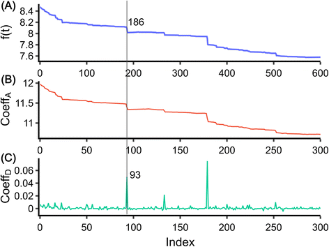 | ||
| Fig. 1 Discrete wavelet transform of the data. (A) Digitized data taken from ref. 22. (B) Approximation coefficient of the data. (C) Detail coefficient of the data. The line shows the step at 186 and a corresponding peak at 93 in the detail coefficient. | ||
2.1. Step detection by wavelet transform
Wavelet transform (WT) is a widely used method for frequency analysis. Similar to the Fourier transform, the WT decomposes a signal into a set of basic functions, known as mother wavelets, at different frequency components.23In our analysis, we used the Discrete Wavelet Transform (DWT), which is governed by the following equation:
 | (1) |
 . The DWT decomposes the target signal into signals of hierarchical frequencies, each half the length of the target signal. This process splits the signal into low and high-frequency components. When these components are summed within their respective groups, two sets of coefficients are obtained. The low-frequency component, known as the approximation coefficient, represents the smooth part of the data (Fig. 1(B)). Conversely, the high-frequency component, known as the detail coefficient, represents areas where the target signals are located (Fig. 1(C)).
To detect the step in the data, we applied the DWT using the Haar mother wavelet. The Haar wavelet, defined as a simple step-shaped function, is particularly effective for this purpose. The mathematical definition of the Haar wavelet is as follows:24,25
 | (2) |
The original signal and its low and high-frequency components, obtained through DWT, are depicted in Fig. 1(A–C). These signals are plotted against the data index, which is the sequence position of the data point. Notably, when there is a step at index i in the original signal, the high-frequency component has a corresponding peak at approximately i/2. The Haar wavelet, representing a signal with sharp changes, is strongly activated at these peaks, effectively capturing the rapid changes in the signal.21 Through DWT, the data are transformed into a signal with peaks that are easier to extract. In contrast to conventional methods that find peaks on the derivative of the target signal, the WT yields detail coefficients close to zero when there are no abrupt changes in the signal. Step detection is accomplished by identifying all the peaks in the detail coefficients without height threshold. The step position in the original signal can be obtained by multiplying the peak indices by two. By setting an appropriate window size (6 indices for the data in Fig. 1, though this value varies with the sampling frequency), a step can be defined as two times the peak indices ± half the window length. This process yields all step-like individual intervals.
To be able to distinguish step signals from noise, we set a height threshold for the identified steps, derived from the calculation of the blocking current (ΔI) using the following equation:22
 | (3) |
2.2. Step detection by deep learning
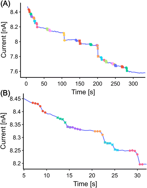
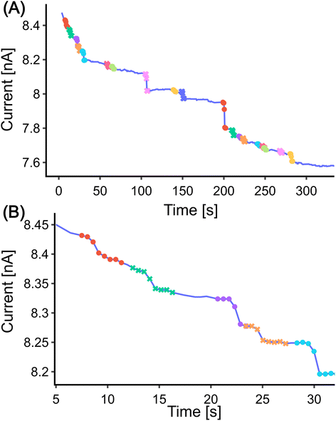
While DWT is an effective method for detecting steps in the data with reasonable precision and speed, it has limitations. Specifically, we found that it would identify any abrupt changes in the current as a step. For instance, in Fig. 2(B), the interval marked in purple is identified as a step despite it not being a true one.To improve the accuracy of the step detection, we incorporated a shallow Convolutional Neural Network (CNN)26 classifier into the algorithm. A CNN can be thought of as a collection of filters. Each filter is a small matrix that performs a convolution operation on the output of the previous layer. These filters are trained to extract features from their input data. The results of these convolutions, which are the extracted features, then serve as the input for the next layer. This process is repeated layer by layer. Eventually, the network outputs a probability value, indicating the likelihood that the input data belongs to a certain class. The workflow for using CNN to detect step signals involves several additional procedures, which are outlined below.
Next, a window length and a step height threshold were defined. This resulted in simulated step intervals. Each step interval was normalized to zero mean and unit variance, as shown in Fig. S1(B).† An equal number of non-step signals (negative signals) were then generated. Each negative signal has the same length as the step interval. Half of the negative signals were created from random Gaussian noise, while the other half were created by introducing an abrupt change point at the initial or final point of the step interval, as shown in Fig. S1(C).† These negative signals are also normalized to zero mean and unit variance. There are approximately 3000 steps and 3000 non-steps in the training set.
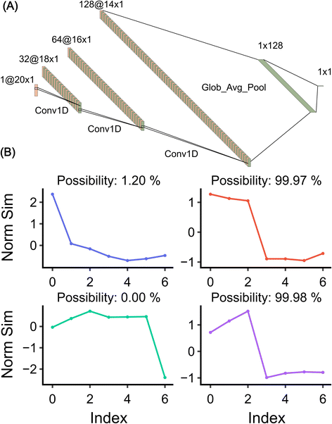 | ||
| Fig. 3 The built CNN model. (A) The CNN model structure. Plotted with ref. 29. (B) Model validation on random signals. The model detects the possibility of whether the signal is a step or not a step. | ||
- Three 1D convolutional layers28 (Conv1–3D in Fig. 3(A)): these layers are designed to extract features from the input data. Each convolutional layer is followed by a batch normalization layer and a dropout layer. The batch normalization layer normalizes the output of the preceding convolutional layer, ensuring that the model trains efficiently. The dropout layer randomly sets a fraction of input units to 0 at each update during training time, which helps prevent overfitting.
- A global average pooling layer (Glob_Avg_Pool in Fig. 3(A)): this layer is added after the last convolutional layer. It reduces the number of parameters in the model, thereby simplifying the model structure and reducing the risk of overfitting. It also transforms the format of the input into a form that can be fed into the dense layer.
- A dense layer with 128 neurons: this layer is added after the global average pooling layer. It uses a ReLU (Rectified Linear Unit) activation function, which introduces non-linearity into the model, allowing it to learn more complex patterns. This layer is followed by another batch normalization layer and a dropout layer.
- A final dense layer: this layer uses a sigmoid activation function, which outputs the probability of the input data to be seen as a step.
The trained model is evaluated on randomly generated data, as shown in Fig. 3(B). The data in the first column incorporate abrupt change, while the data in the second column contain a step. As can be seen, the model predicts well the possibility of the signal being a step and, contrary to DWT, does not misassign an abrupt change to a step signal.
The detected steps were merged if the initial point and the maximum difference point of the current step and the next step were within 10% of the height threshold. If two steps were not qualified to be merged but the index of the initial point of the next step was within the current step, the overlapped points were averaged.
2.3. Data extraction
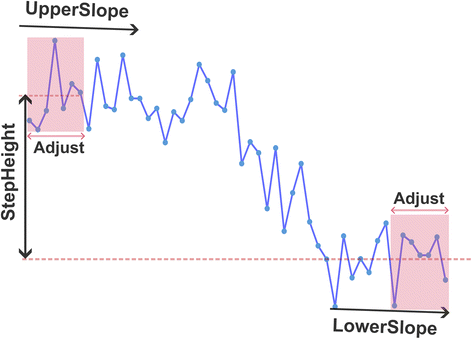
Both methods can be used to analyse the data. We extracted key parameters from each step interval that both methods detected. These extracted parameters are illustrated in Scheme 1. The parameters include ‘UpperSlope’ and ‘LowerSlope’, which are calculated from the slopes of the first two and last two points of the step interval, respectively. ‘StepHeight’ is calculated as the difference between the mean values of the first two and last two points of the step interval.As the sampling frequency rises, the number of data points required for parameter extraction also increases. For low-frequency signals, a minimal number of points are used for calculation to ensure exclusion of the decay portion of the step. For signals with a higher sampling frequency, the quantity of data points selected for parameters extraction is increased to accommodate the increased data density (see Section 2.4). The parameters extracted from the initial 32 seconds of data using both methodologies are detailed in Table S1.†
At this stage, we can make a preliminary comparison between the two methods. The CNN method detected three fewer steps than the DWT method when using the same height threshold. Three false positives detected by the DWT method are due to its sensitivity to a sudden value change which is not necessarily a step (Fig. 2(B) marked with purple). The CNN method, on the other hand, is more robust in detecting steps. It only identifies a step when the upper and lower parts of the signal match a certain profile. Moreover, it offers more flexibility in terms of the shapes it can detect, as the training set can be adjusted to include more complex step shapes.
However, the CNN method requires more computational resources and time. For the same signal, the DWT method takes less than 1 second, while CNN needs background knowledge, and the training process requires higher computation costs. As the sampling frequency increases, the time required for the CNN method to detect steps also increases. Therefore, when choosing a detection method, there is a trade-off between accuracy and computational complexity.
To further analyse the data and compare the two methods, we employed a k-means unsupervised machine learning method.7 This method was used to cluster the ‘UpperSlope’, ‘LowerSlope’, and ‘StepHeight’ parameters. The optimal number of clusters was determined using the elbow method. We then compared the results of this clustering for the two detection methods mentioned earlier. The results are depicted in Fig. 5. In the 3D space, both methods form distinct clusters.30 However, the clusters generated by the DWT have larger variance compared to those from the CNN method, indicating that the CNN method has higher precision.
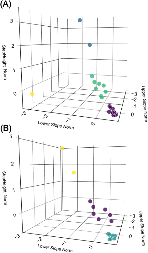 | ||
| Fig. 5 3D plots comparing data clustered by k-means (colour coded), the 3 dimensions StepHeight, UpperSlope, and LowerSlope are separately normalized. (A) The DWT method. (B) The CNN method. | ||
2.4. Validation
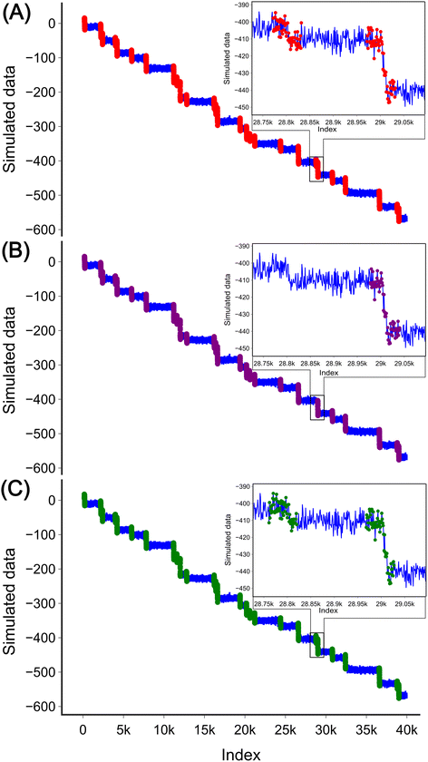
To evaluate the applicability of these two methods to experimental data which are often characterised by the high sampling frequency and more complex step shapes,31,32 we simulated a signal with 40![[thin space (1/6-em)]](https://www.rsc.org/images/entities/char_2009.gif) 000 data points containing 30 steps marked with red (Fig. 6(A)). The steps in the data with the high-frequency sampling have different profiles compared to those in the low-frequency data used for the analysis method development. In low-frequency measurements, a step can be simply defined as a current value dropping from one nearly fixed value to another. However, in high-frequency measurements, the upper fixed value decays with a certain slope to the lower fixed value, and both the upper and lower sides have additional slope and high noise. This complexity leads to the step being less well defined. In addition to the evident steps, there are also some steps with a height nearly equal to the noise level. Three such steps were therefore filtered out at this stage as they were difficult to distinguish from the noise resulting in 27 steps in total.
000 data points containing 30 steps marked with red (Fig. 6(A)). The steps in the data with the high-frequency sampling have different profiles compared to those in the low-frequency data used for the analysis method development. In low-frequency measurements, a step can be simply defined as a current value dropping from one nearly fixed value to another. However, in high-frequency measurements, the upper fixed value decays with a certain slope to the lower fixed value, and both the upper and lower sides have additional slope and high noise. This complexity leads to the step being less well defined. In addition to the evident steps, there are also some steps with a height nearly equal to the noise level. Three such steps were therefore filtered out at this stage as they were difficult to distinguish from the noise resulting in 27 steps in total.
At high sampling frequencies, step detection becomes more challenging. Traditional methods, such as derivative detection, are no longer effective, as evidenced by the lack of clear peaks in the derivative shown in Fig. S3.† However, both methods developed in this study are capable of detecting the steps in such cases.
For the DWT, a single transform is no longer effective in detecting the steps. After three transforms, the spikes corresponding to the steps start to become visible (Fig. S4(E)†), and after five transforms, the spikes are clearly visible, as shown in Fig. S4(G).† Similar to low frequency data analysis all peaks were detected without height threshold. Each step interval was defined as the index on the original signal minus half the window length, plus 1.5 times the half window size. In this example, we used 60 as the window size, so an interval is defined as [index − 15, index + 45] to cover the long decay of the steps. By defining the height threshold for the step as 7 units (the value was chosen based on how the data for analysis were simulated), 26 steps were detected in the data, as shown in Fig. 6(B). One of the steps was missed by the method (inset in Fig. 6(B)). It is important to note that when applying the DWT method to a new data set the number of transforms needs to be adjusted. As the number of transforms increases, the loss of the high-frequency components may contain the desired steps.
For the CNN method step detection can be achieved by modifying the training set and slightly adjusting the structure of the model. The training set is shown in Fig. S5.† The fundamental structure of the CNN model remains unchanged, with the only modification being the adjustment of the input layer to 60 to accommodate the requirements of the input data, as the sequential layer output numbers vary accordingly. The model was trained for 300 epochs to facilitate easier adjustment of the decay length of the training set. The progression of the training set is depicted in Fig. S6(A).† The trained model is similar to the model used for the low-frequency data analysis (Fig. 3), with the exception that it neglects steps located at the beginning or end of the window Fig. S6(B).† This model was then applied to the high-frequency simulated data. Similar to low-frequency data analysis, the model was slid across the experimental data by iterating through all the data points. Each interval, with a window length of 60, was normalized to zero mean and unit variance. If the probability of a step exceeded 0.5, it was considered as a step. Interestingly, the model no longer requires height thresholding for detection. This may be due to the fact that the shape of the step was well trained in the training process. 27 steps were detected in total with the CNN model as shown in Fig. 6(C).
For each detected step, three parameters were extracted as outlined in Scheme 1. Similar to the low-frequency data, the ‘StepHeight’ is calculated as the mean difference between the first five points and the last five points within the step interval. The ‘UpperSlope’ and ‘LowerSlope’ parameters are calculated as the slope of the first ten points and the last ten points of the step interval, respectively. The parameters extracted by both methods are presented in Table S2.†
3. Conclusions
Here we presented two methods for detecting steps in single-entity electrochemistry data. Both developed methods, DWT and CNN, can be used for data analysis of both low- and high-frequency data. The DWT method is computationally efficient and direct, but it often requires post-processing. Moreover, the height threshold is a critical factor for step detection with the DWT. On the other hand, the CNN method, while more accurate and robust, requires more computational resources. For instance, for the high-frequency data with 40![[thin space (1/6-em)]](https://www.rsc.org/images/entities/char_2009.gif) 000 data points, the CNN method required twice the computational time of the DWT method (less than 1 second for DWT, and about 2 seconds for CNN). Additionally, the CNN method needs additional time to prepare the training set and train the model. The CNN method offers more flexibility in terms of the shapes it can detect, as the training set can be adjusted to include more complex step shapes. However, if the desired signal cannot be well simulated, the results obtained with the CNN method may not be satisfactory. Therefore, well-simulated physical data or real data should be used to train the CNN model.
000 data points, the CNN method required twice the computational time of the DWT method (less than 1 second for DWT, and about 2 seconds for CNN). Additionally, the CNN method needs additional time to prepare the training set and train the model. The CNN method offers more flexibility in terms of the shapes it can detect, as the training set can be adjusted to include more complex step shapes. However, if the desired signal cannot be well simulated, the results obtained with the CNN method may not be satisfactory. Therefore, well-simulated physical data or real data should be used to train the CNN model.
4. Experimental
4.1. Modules and software
The data used for the development of the methods were digitized from ref. 22 using the GitHub package PlotDigitizer.33 It is important to note that the digitized signal may not fully represent the original signal, particularly in terms of the sampling frequency. For method development Python packages such as NumPy,34 SciPy,35 pandas,36 and scikit-learn37 were used. The wavelet transform was carried out using the PyWavelets38 package on an Intel 12700H CPU. The CNN was implemented using the TensorFlow39 Keras package, running on a laptop with a 60W RTX 3060 GPU. For data visualisation, the Plotly40 package was used. The scripts used in this study are available on the GitHub repository at https://github.com/ziwzh166/SEE_StepAnalysis.Data availability
Data for this article, including the corresponding scripts, are available at Github SEE_StepAnalysis at https://github.com/ziwzh166/SEE_StepAnalysis.Author contributions
Z. Z.: conceptualization, methodology, software, validation, data curation, writing – original draft, visualization; A. N.: methodology, software; N. K.: methodology; A. S.: conceptualization, writing – review and editing, supervision.Conflicts of interest
There are no conflicts to declare.Acknowledgements
The authors greatly acknowledge Petko Chernev at Uppsala University for his efforts in coding the interface for chronoamperometry measurements in the Keithley sourcemeter. A. S. thanks the Swedish Research Council (grant number 2020-03262) and the Göran Gustafsson Foundation (grant number 2320).Notes and references
- B. M. Quinn, P. G. van’t Hof and S. G. Lemay, J. Am. Chem. Soc., 2004, 126, 8360–8361 CrossRef CAS PubMed.
- X. Xiao and A. J. Bard, J. Am. Chem. Soc., 2007, 129, 9610–9612 CrossRef CAS.
- Y.-G. Zhou, N. V. Rees and R. G. Compton, Angew. Chem., Int. Ed., 2011, 50, 4219–4221 CrossRef CAS PubMed.
- A. N. Sekretaryova, M. Y. Vagin, A. P. F. Turner and M. Eriksson, J. Am. Chem. Soc., 2016, 138, 2504–2507 CrossRef CAS PubMed.
- L. A. Baker, J. Am. Chem. Soc., 2018, 140, 15549–15559 CrossRef CAS.
- X. Li, Y.-H. Fu, N. Wei, R.-J. Yu, H. Bhatti, L. Zhang, F. Yan, F. Xia, A. G. Ewing, Y.-T. Long and Y.-L. Ying, Angew. Chem., Int. Ed., 2024, 63, e202316551 CrossRef CAS.
- Z. Zhao, A. Naha, S. Ganguli and A. Sekretareva, Adv. Intell. Syst., 2024, 6, 2300424 CrossRef.
- S. J. Kwon, H. Zhou, F.-R. F. Fan, V. Vorobyev, B. Zhang and A. J. Bard, Phys. Chem. Chem. Phys., 2011, 13, 5394–5402 RSC.
- A. Sekretareva, Sens. Actuators Rep., 2021, 3, 100037 CrossRef.
- C. Tyson, C. McAndrew, P. L. Tuma, I. Pegg and A. Sarkar, Cytometry, Part A, 2015, 87, 393–404 CrossRef CAS.
- A. Moghaddamjoo, IEEE Trans. Ind. Electron., 1988, 35, 489–493 CrossRef.
- B. Kalafut and K. Visscher, Comput. Phys. Commun., 2008, 179, 716–723 CrossRef CAS.
- N. J. Carter and R. A. Cross, Nature, 2005, 435, 308–312 CrossRef CAS.
- J. W. J. Kerssemakers, E. Laura Munteanu, L. Laan, T. L. Noetzel, M. E. Janson and M. Dogterom, Nature, 2006, 442, 709–712 CrossRef CAS PubMed.
- S. G. Arunajadai and W. Cheng, PLoS One, 2013, 8, e59279 CrossRef CAS PubMed.
- J. H. Forstater, K. Briggs, J. W. F. Robertson, J. Ettedgui, O. Marie-Rose, C. Vaz, J. J. Kasianowicz, V. Tabard-Cossa and A. Balijepalli, Anal. Chem., 2016, 88, 11900–11907 CrossRef CAS.
- C. Raillon, P. Granjon, M. Graf, L. J. Steinbock and A. Radenovic, Nanoscale, 2012, 4, 4916–4924 RSC.
- Z. Gu, Y.-L. Ying, C. Cao, P. He and Y.-T. Long, Anal. Chem., 2015, 87, 907–913 CrossRef CAS PubMed.
- C. Wen, D. Dematties and S.-L. Zhang, ACS Sens., 2021, 6, 3536–3555 CrossRef CAS.
- Á. Díaz Carral, M. Ostertag and M. Fyta, J. Chem. Phys., 2021, 154, 044111 CrossRef.
- B. M. Sadler and A. Swami, Analysis of Wavelet Transform Multiscale Products for Step Detection and Estimation, Defense Technical Information Center, Fort Belvoir, VA, 1998 Search PubMed.
- J. E. Dick, C. Renault and A. J. Bard, J. Am. Chem. Soc., 2015, 137, 8376–8379 CrossRef CAS PubMed.
- Data-Driven Science and Engineering: Machine Learning, Dynamical Systems, and Control, ed. J. N. Kutz and S. L. Brunton, Cambridge University Press, Cambridge, 2019, pp. 47–83 Search PubMed.
- A. Haar, Math. Ann., 1910, 69, 331–371 CrossRef.
- B. Y. Lee and Y. S., Int. J.Adv. Manuf. Technol., 1999, 15, 238–243 CrossRef.
- Y. LeCun, Y. Bengio and G. Hinton, Nature, 2015, 521, 436–444 CrossRef CAS.
- keras-team/keras, Keras, 2024 Search PubMed.
- S. Kiranyaz, T. Ince, O. Abdeljaber, O. Avci and M. Gabbouj, in ICASSP 2019 – 2019 IEEE International Conference on Acoustics, Speech and Signal Processing, ICASSP, 2019, pp. 8360–8364 Search PubMed.
- A. LeNail, J. Open Source Softw., 2019, 4, 747 CrossRef.
- A. Ameur, J. Dahlberg, P. Olason, F. Vezzi, R. Karlsson, M. Martin, J. Viklund, A. K. Kähäri, P. Lundin, H. Che, J. Thutkawkorapin, J. Eisfeldt, S. Lampa, M. Dahlberg, J. Hagberg, N. Jareborg, U. Liljedahl, I. Jonasson, Å. Johansson, L. Feuk, J. Lundeberg, A.-C. Syvänen, S. Lundin, D. Nilsson, B. Nystedt, P. K. Magnusson and U. Gyllensten, Eur. J. Hum. Genet., 2017, 25, 1253–1260 CAS.
- Q. Wang, J. Lin, S. Li, H. Tian, D. Zhang and Q. Xin, Anal. Chem., 2023, 95, 13082–13090 CrossRef CAS.
- S. E. Alden, L. Zhang, Y. Wang, N. V. Lavrik, S. N. Thorgaard and L. A. Baker, Anal. Chem., 2024, 96, 9177–9184 CrossRef CAS PubMed.
- D. Singh, dilawar/PlotDigitizer, 2024, https://github.com/dilawar/PlotDigitizer Search PubMed.
- C. R. Harris, K. J. Millman, S. J. van der Walt, R. Gommers, P. Virtanen, D. Cournapeau, E. Wieser, J. Taylor, S. Berg, N. J. Smith, R. Kern, M. Picus, S. Hoyer, M. H. van Kerkwijk, M. Brett, A. Haldane, J. F. del Río, M. Wiebe, P. Peterson, P. Gérard-Marchant, K. Sheppard, T. Reddy, W. Weckesser, H. Abbasi, C. Gohlke and T. E. Oliphant, Nature, 2020, 585, 357–362 CrossRef CAS PubMed.
- P. Virtanen, R. Gommers, T. E. Oliphant, M. Haberland, T. Reddy, D. Cournapeau, E. Burovski, P. Peterson, W. Weckesser, J. Bright, S. J. van der Walt, M. Brett, J. Wilson, K. J. Millman, N. Mayorov, A. R. J. Nelson, E. Jones, R. Kern, E. Larson, C. J. Carey, İ. Polat, Y. Feng, E. W. Moore, J. VanderPlas, D. Laxalde, J. Perktold, R. Cimrman, I. Henriksen, E. A. Quintero, C. R. Harris, A. M. Archibald, A. H. Ribeiro, F. Pedregosa and P. van Mulbregt, Nat. Methods, 2020, 17, 261–272 CrossRef CAS PubMed.
- T. pandas development team, pandas-dev/pandas (version v2.2.2), Zenodo, 2024 Search PubMed.
- F. Pedregosa, et al. , J. Mach. Learn. Res., 2011, 12, 2825–2830 Search PubMed.
- G. R. Lee, R. Gommers, F. Waselewski, K. Wohlfahrt and A. O’Leary, J. Open Source Softw., 2019, 4, 1237 CrossRef.
- T. Developers, TensorFlow (version v2.15.1), Zenodo, 2024 Search PubMed.
- Data Apps for Production, Plotly, https://plotly.com/ Search PubMed.
Footnote |
| † Electronic supplementary information (ESI) available. See DOI: https://doi.org/10.1039/d4fd00130c |
| This journal is © The Royal Society of Chemistry 2025 |

