 Open Access Article
Creative Commons Attribution 3.0 Unported Licence
Inverse design of copolymers including stoichiometry and chain architecture
Gabriel
Vogel
 and
Jana M.
Weber
 *
*
Department of Intelligent Systems, Delft University of Technology, Delft 2629 HZ, The Netherlands. E-mail: j.m.weber@tudelft.nl
First published on 17th December 2024
Abstract
The demand for innovative synthetic polymers with improved properties is high, but their structural complexity and vast design space hinder rapid discovery. Machine learning-guided molecular design is a promising approach to accelerate polymer discovery. However, the scarcity of labeled polymer data and the complex hierarchical structure of synthetic polymers make generative design particularly challenging. We advance the current state-of-the-art approaches to generate not only repeating units, but monomer ensembles including their stoichiometry and chain architecture. We build upon a recent polymer representation that includes stoichiometries and chain architectures of monomer ensembles and develop a novel variational autoencoder (VAE) architecture encoding a graph and decoding a string. Using a semi-supervised setup, we enable the handling of partly labelled datasets which can be beneficial for domains with a small corpus of labelled data. Our model learns a continuous, well organized latent space (LS) that enables de novo generation of copolymer structures including different monomer stoichiometries and chain architectures. In an inverse design case study, we demonstrate our model for in silico discovery of novel conjugated copolymer photocatalysts for hydrogen production using optimization of the polymer's electron affinity and ionization potential in the latent space.
1 Introduction
Polymers have evolved into a cornerstone of modern society, finding applications across diverse domains such as food packaging,1 textiles,2 photovoltaics,3 clinical medicine,4 and many more. As the demand for innovative polymers surges, researchers face the task of navigating a vast design space. The space is uniquely characterized by the complexity of polymer materials which span from the chemical structure of monomers to diverse topologies and morphologies of the polymer material. Traditionally, polymer design relies heavily on expert knowledge and trial-and-error of selected real-world experiments in the lab and in silico simulations. Recently, machine learning (ML) has increasingly contributed to polymer informatics,5,6 aiming to develop efficient strategies for polymer design. The core idea is to learn from existing polymer data, implicitly leveraging expert knowledge, to navigate the vast design space and find promising polymer candidates. These candidates can then be evaluated through in silico experiments and synthesized and tested in the lab.There are two prominent ML-based strategies to accelerate the discovery of new molecules7–10 also applicable to polymers. First, in direct design strategies,11,12 ML models are trained to learn polymer structure-to-property relationships from known labelled polymer data. This approach can be used for virtual screening of polymer structure libraries to find the candidate with the best predicted properties. This provides an efficient way to limit the number of experiments. However, this approach is constrained by a selection bias of predefined polymer structures to test, only focusing on a very small fraction of the full design space. In response, in inverse design strategies8,13 generative models are specifically trained to generate novel polymer structures with desired properties. One advantage of this approach is that candidate polymer structures do not need to be defined upfront. Labelled data and knowledge of the optimal property value is however still required. If trained correctly, this approach allows for iteratively optimizing toward novel polymers (not in the data library) with optimal properties (properties beyond the best values in the library). This can for instance be achieved through the combination of the generative model with optimization algorithms such as Bayesian optimization or genetic algorithms. In this work, we focus on the inverse design of polymers using generative modelling.
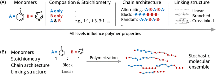
An inverse design model requires a machine-readable representation that accurately captures the molecular structure and further can be generated by a generative model. This is especially challenging for polymers. Polymers possess a hierarchical structure spanning from the monomer chemistry to the polymer morphology. To a certain extent, all levels indicated in Fig. 1(A) impact the material's properties. At the smallest scale, polymers consist of monomer units with varying stoichiometries. Depending on the polymerization type and the reaction/processing conditions, the monomers can be arranged in diverse chain architectures, which are often described as polymer topologies. For instance, simply linear topologies with alternating, block, random, or other monomer arrangements exist. Other examples are lightly branched chains,14 hyperbranched,15 cyclic16 or star-shaped17 polymer topologies. Further, the processing conditions influence morphological traits such as crystallinity and therewith also the properties.6 Besides, many polymers are stochastic. That means that they are ensembles of macromolecules of differing sizes and weights (see Fig. 1(B)), which complicates the use of just one single polymer representation.
Numerous studies have employed descriptor-based fingerprinting in different variations to represent polymers as numerical vectors (see a comprehensive overview by Yan and Li5). Polymer fingerprints have been widely used for predicting polymer properties,18–22 however and most notably, fingerprints are unsuitable for generative design. This is due to their non-invertibility, meaning that they cannot be uniquely mapped back and forth between the actual molecule and the fingerprint. In contrast, string and graph-based representations are invertible and thus appropriate for generative design.
Most string-based polymer representations, such as pSMILES,23,24 build upon the SMILES (Simplified Molecule Line Entry System) notation, adapting it for polymers by incorporating the repeating unit's SMILES and connection points using the * symbol. The pSMILES (or similar variants) has been used widely for the prediction of mechanical, thermal, thermodynamical, electronical and optical properties.25,26 Moreover, it has been used to discover novel polymer structures with generative models.23,27–29 While pSMILES efficiently describes repeat unit chemistries, it falls short in depicting monomer combinations, higher-order structures, and polymer stochasticity. BigSMILES, an extension by Lin et al.,30 offers greater flexibility, describing polymers as stochastic objects, accommodating multiple monomers and their connection points. However, BigSMILES lacks encoding for stoichiometry and processing history. G-BigSMILES,31 a recent work, extends the BigSMILES to include molecular weight distributions and connection probabilities, indirectly capturing monomer stoichiometry. The recent advances in the string-based polymer representations show promise for the development of more precise inverse design models, however these advanced representations have not yet been employed with generative models.
Most polymer graph representations are simplified using only the molecular graph of one monomer or repeat unit.32 This can be applied for property prediction but also for generative design as shown in the work by Liu et al.33 Recent works aim to move towards polymer graphs that represent macromolecules instead of only the repeat unit. One proposed approach known as PolyGrammar34 makes use of hypergraphs to represent polymeric structures by explicitly defining sequences of monomers. It enables describing complex chain architectures and allows for generative design approaches, but does not account for the stochastic nature of polymer materials. Other approaches approximate the macromolecule by adding an additional edge (loop) between the connection points of the repeating unit.35,36 Moreover, Aldeghi and Coley37 introduced a polymer graph that comprises multiple monomers as subgraphs, which are interconnected by additional weighted edges. The introduction of weighted edges enables the authors to capture the stochastic nature of polymer as monomer ensembles and facilitates the description of diverse polymer types (e.g., homo- and copolymers including stoichiometry) and various chain architectures (such as alternating, block, random, and graft structures).
Given the impact of structural and stochastic variability beyond the repeat unit on polymer properties, we believe that incorporating these factors is key to accurate inverse design of property-optimized polymers. Our work addresses this challenge. We build upon the recent graph representation37 and use a Graph-2-string Variational Autoencoder38 for inverse design of copolymers. Our work generates polymers defined by their monomer chemistries, monomer stoichiometry, and chain architecture. We lead our generative model towards the design of optimal polymers through two steps. Firstly, we present a semi-supervised VAE setup to enable working with partly labelled and unlabelled data. Secondly, we employ two molecular optimisation strategies in the continuous latent space, which were previously demonstrated successfully in the literature.39,40 We illustrate our approach in a case study for the in silico discovery of novel photocatalysts for green hydrogen production.
2 Methods
This section first explains the employed graph and text-based polymer representations briefly. Afterwards, we outline the general concept of VAEs and explain the detailed model architecture of the semi-supervised Graph-2-string VAE developed in this work. We then introduce the case study and dataset of copolymer photocatalysts for hydrogen production. Furthermore, we explain the evaluation metrics and conclude with details on the optimization in latent space.2.1 Polymer representations
Our approach integrates graph- and string-based representations, as depicted in Fig. 2. Both represent the polymers as stochastic ensembles, including stoichiometry and chain architecture information. | ||
| Fig. 2 Polymer representations accounting for stoichiometry of monomer ensembles, the chain architecture and the stochastic nature of polymers. The graph representation is adopted from Aldeghi and Coley,37 with stochastic edges (dashed) reflecting the connection probabilities between monomers, i.e. reflecting the chain architecture. The string representation is a text-based description of the polymer graph representation, concatenating monomer SMILES, stoichiometry and connection probabilities. | ||
2.2 Model
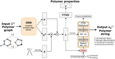
We build on the general framework of a variational autoencoder (VAE),42 a probabilistic generative model. This model consists of an encoder network qϕ(z|x) that maps high-dimensional data x to a latent space distribution z, which is approximated by a Gaussian distribution with mean μ and variance σ2. Additionally, it includes a decoder network pθ(x|z) that maps samples from the latent space z back to the data space, aiming to reconstruct the original input x.To encode a polymer graph we re-implement the proposed weighted directed edge message passing neural network (wD-MPNN).37 We use one wD-MPNN block with 3 layers and subsequently two parallel blocks that output a mean μ and variance σ2 vector, respectively.38 Then we use the reparametrization trick42 to obtain the latent embedding z.
The latent embedding is fed to a Transformer-based45 language model consisting of four sequential layers with each four attention heads to decode the equivalent polymer string. In addition to the encoder-decoder cross attention between z and previously generated token embeddings, we concatenate z with each token embedding after the positional encoding, slightly different to Fang et al.46 who added it element wise. This was motivated by work in the natural language domain showing that the combination of VAEs and a transformer decoder requires modifications that regulate how the latent space is fed to the decoder.46,47 This modification improved the reconstruction ability of the model substantially as demonstrated in ref. 38.
We further include knowledge about the properties in our model to generate a property-organised latent space. We adopt the approach of Gómez-Bombarelli et al.48 that adds an additional feed-forward neural network taking the latent embedding z as input to predict a property y (or multiple) that is jointly trained with the VAE architecture consisting of encoder and decoder networks.
 , Kullback-Leibler divergence loss
  and an additional property loss term
  . For additional details on the derivation of the loss see Appendix A.1.2. We further use two hyperparameters β and α to balance the loss terms.
 | (1) |
 is calculated as the weighted cross entropy loss between the ground truth and predicted polymer string given the latent representation z. Further, as will be outlined in Section 2.3, we have a combination of labelled and unlabelled data. To handle partially labelled data, we introduce a mask m for the property loss
 | (2) |
 | (3) |
2.3 Case study and dataset
We test our model in a case study to design novel conjugated copolymers which are emerging as promising organic photocatalysts for green hydrogen production through photocatalytic water splitting. The process involves a photocatalyst that absorbs light to generate charge carriers which reduce protons to hydrogen while oxidizing water or an electron donor. Addressing the vast synthetic diversity of conjugated polymers, Bai et al.49 conducted a high-throughput screening study to explore various copolymers, analyzing their hydrogen evolution rate (HER) as a measure of photocatalytic activity. Ultimately, we aim to find candidate polymers with improved catalytic activity (see Sections 2.5 and 3.4).We base our study on the dataset introduced by Aldeghi and Coley37 which is built upon the conjugated copolymer space of Bai et al.49 As shown in Fig. 4, the dataset combines eight A-monomers with 682 B-monomers in stoichiometries of 1![[thin space (1/6-em)]](https://www.rsc.org/images/entities/char_2009.gif) :
:![[thin space (1/6-em)]](https://www.rsc.org/images/entities/char_2009.gif) 1, 1
1, 1![[thin space (1/6-em)]](https://www.rsc.org/images/entities/char_2009.gif) :
:![[thin space (1/6-em)]](https://www.rsc.org/images/entities/char_2009.gif) 3, and 3
3, and 3![[thin space (1/6-em)]](https://www.rsc.org/images/entities/char_2009.gif) :
:![[thin space (1/6-em)]](https://www.rsc.org/images/entities/char_2009.gif) 1 and three types of chain architectures (alternating, random, block). This leads to 42
1 and three types of chain architectures (alternating, random, block). This leads to 42![[thin space (1/6-em)]](https://www.rsc.org/images/entities/char_2009.gif) 966 copolymers. The dataset additionally reports the ionization potential (IP) and electron affinity (EA), determined with DFT calculations for all 42
966 copolymers. The dataset additionally reports the ionization potential (IP) and electron affinity (EA), determined with DFT calculations for all 42![[thin space (1/6-em)]](https://www.rsc.org/images/entities/char_2009.gif) 966 polymer candidates.37 Additionally, we construct an augmented version of the data set, allowing for B–B copolymers to increase the diversity of the chemical space of monomer A. We combine each of the 682 B monomers with 20 randomly selected B monomers across 7 stoichiometry-chain architecture combinations. This adds 682 × 20 × 7 = 95
966 polymer candidates.37 Additionally, we construct an augmented version of the data set, allowing for B–B copolymers to increase the diversity of the chemical space of monomer A. We combine each of the 682 B monomers with 20 randomly selected B monomers across 7 stoichiometry-chain architecture combinations. This adds 682 × 20 × 7 = 95![[thin space (1/6-em)]](https://www.rsc.org/images/entities/char_2009.gif) 480 new data points, resulting in a total of 138
480 new data points, resulting in a total of 138![[thin space (1/6-em)]](https://www.rsc.org/images/entities/char_2009.gif) 446 points (ca. 3× the size of the original dataset). The labels IP and EA are only available for the original data points, hence, we obtain a partly labelled dataset.
446 points (ca. 3× the size of the original dataset). The labels IP and EA are only available for the original data points, hence, we obtain a partly labelled dataset.
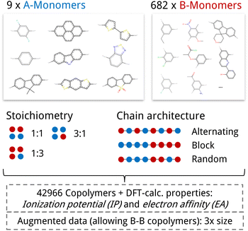 | ||
Fig. 4 Copolymer photocatalyst dataset from Aldeghi and Coley37 that is used in this work. The polymer space consists of 9 A-monomers and 682 B-monomers that are combined in three stoichiometries (1![[thin space (1/6-em)]](https://www.rsc.org/images/entities/char_2009.gif) : :![[thin space (1/6-em)]](https://www.rsc.org/images/entities/char_2009.gif) 1, 1 1, 1![[thin space (1/6-em)]](https://www.rsc.org/images/entities/char_2009.gif) : :![[thin space (1/6-em)]](https://www.rsc.org/images/entities/char_2009.gif) 3, 3 3, 3![[thin space (1/6-em)]](https://www.rsc.org/images/entities/char_2009.gif) : :![[thin space (1/6-em)]](https://www.rsc.org/images/entities/char_2009.gif) 1) and three chain architectures (alternating, block, random). This forms a dataset of 42 1) and three chain architectures (alternating, block, random). This forms a dataset of 42![[thin space (1/6-em)]](https://www.rsc.org/images/entities/char_2009.gif) 966 copolymers, including DFT-calculated polymer properties ionization potential (IP) and electron affinity (EA). We create an augmented data set without the property labels (ca. 3 times the size) by allowing the combination of B–B copolymers. 966 copolymers, including DFT-calculated polymer properties ionization potential (IP) and electron affinity (EA). We create an augmented data set without the property labels (ca. 3 times the size) by allowing the combination of B–B copolymers. | ||
2.4 Training and evaluation
We split the dataset in 80% training data, and 10% validation and 10% test data. Since we have multiple data points per monomer combination (varying stoichiomtry and chain architecture), we split the data by monomer combinations to prevent data leakage, i.e. ensuring that there are no monomer combinations in the test- or validation set that also occur in the training set. During training we apply the default teacher forcing in the Transformer decoder and use early stopping based on the evaluation on the held out validation set. During inference, i.e. the novel generation of polymers from latent embeddings z, we use beam search with a beam size of five to decode the polymer strings. This maximizes the final probability of the sequence and helps with generating valid SMILES. Where applicable, we adopted the hyperparameters of Vogel et al.,38 which is the unsupervised version (only encoder and decoder) of the model used in this work. To ensure a more stable training we use a cyclical schedule for β.50 Additionally, we performed a hyperparameter search over β and α to balance the contribution of the loss terms in eqn (2). Note, that we limited the hyperparameter search of these parameters to a fixed number of evaluations in a random search approach and subsequent fine-grained grid search.During the hyperparameter search and to assess the final model performance, we calculate quantitative metrics that have been established in the small molecule domain: reconstruction, validity, novelty, and uniqueness, defined in Table 1. Reconstruction is evaluated on the test set, encoding each sample to a latent point z = μ and passing it to the decoder to produce the polymer string representation. Novelty and Uniqueness are evaluated for the sampled set which consists of 16![[thin space (1/6-em)]](https://www.rsc.org/images/entities/char_2009.gif) 000 polymers randomly sampled from Gaussian noise. Validity is calculated both for the reconstructed test set as well as the sampled set. In the results in Section 3 we use the best performing model according to these model metrics and qualitative assessments of the latent space structure. In Section 3.3 we explain in more detail how we combine the quantitative and qualitative assessment.
000 polymers randomly sampled from Gaussian noise. Validity is calculated both for the reconstructed test set as well as the sampled set. In the results in Section 3 we use the best performing model according to these model metrics and qualitative assessments of the latent space structure. In Section 3.3 we explain in more detail how we combine the quantitative and qualitative assessment.
![[thin space (1/6-em)]](https://www.rsc.org/images/entities/char_2009.gif) 000 polymers sampled from Gaussian noise
000 polymers sampled from Gaussian noise
2.5 Property optimization and inverse design
To generate polymers with desired properties, we employ optimization in the numerical latent space of our trained VAE model. We define the 32 numerical latent dimensions as input variables for an optimization algorithm, denoted as z = {z1, z2, …, z32}. The objective function is composed of target values for the predicted copolymer properties from the latent space. The ideal scenario would be to maximize for the HER, however, this property is not reported for the dataset we used to train our model. We use the observation,49 that the two electronic properties IP and EA are correlated to the HER of copolymer catalysts. Optimal target values for IP and EA can be derived for instance using expert knowledge, targeting a specific chemical region that is known to perform well (see Appendix B.1.4 and B.1.5), or through observed trends in high-throughput studies. Hereinafter, we used the last option, deriving target values of EA and IP from the analysis in Bai et al.49Bai et al.49 found that, overall, materials with high HERs tend to have larger optical gaps, more negative EA values, and an IP of around 1 eV. Given the common approximation for the optical gap as |EA – IP|, minimizing the EA while keeping IP fixed also maximizes the optical gap. Based on these findings, we reason that IP ≈ 1 and more negative values of EA are indicative of better HERs and thus correlate to better photocatalytic performance (see also Appendix A.1.3). Consequently, we seek to minimize the overall objective function f(z):
| f(z) = |ppIP(z) − 1| + ppEA(z) + peninv(xS). | (4) |
Note that, since we are not optimizing for HER directly, other objective values for EA and IP (see, Appendix B.1.5) could also serve as effective strategies for identifying high-performing photocatalysts.
| UCB(z;κ) = μ(z) + κσ(z), | (5) |
To address this, we designed an approach aimed at ensuring high confidence in property predictions ppIP(z) and ppEA(z). This involves correcting points sampled by BO, denoted as zBO, by decoding and re-encoding them to obtain z′ ≈ zBO. Consequently, we ensure that the point lies within a high-confidence region of the latent space, suitable as input to the property predictor network. Thus, we achieve more accurate property predictions (see also Appendix B.1.3), which mitigates discrepancies between the predicted properties used for objective function evaluations and the corresponding decoded polymers.
To tackle the problem of low-confidence regions in the latent space we implement a repair mechanism after the offsprings (new individuals after crossover and mutation) have been reproduced. We adjust these offsprings zoffspring, by decoding and re-encoding them to obtain  to ensure they are within high-density regions of the latent space. These points are then evaluated to calculate the objectives.
3 Results and discussion
In this section we demonstrate the generative capabilities of our model to generate novel copolymers including their stoichiometry and chain architecture. We first assess the overall model performance as a generative model in terms of reconstruction and validity, novelty, and uniqueness of sampled polymers. Further, we analyse the structure and smoothness of the latent space qualitatively. Then we test our model for inverse design of property-optimized organic copolymer photocatalysts for improved green hydrogen production.3.1 Model evaluation
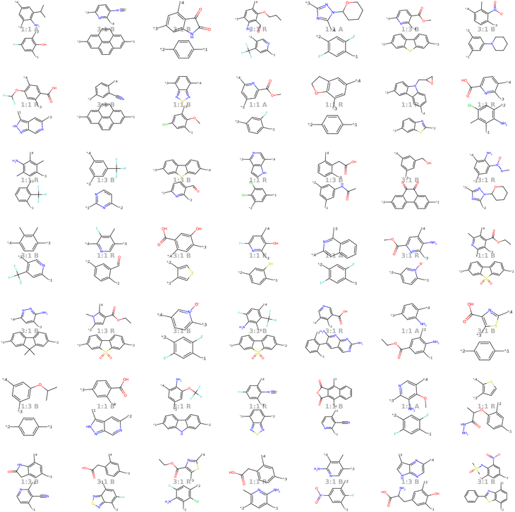
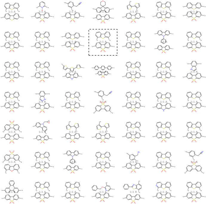
Our model demonstrates good performance in generating novel, diverse, and chemically valid polymers and reconstructing complex copolymer structures. With the best hyperparameter configuration (see Section 3.3) we achieve a reconstruction accuracy of 68% for copolymers in the testset, including their higher-order structural information (chain architecture and stoichiometry). Further, the model generates novel (81%) and unique (98%) polymers. The reconstructed test set exhibits 99% valid and the generated sample set 96% chemically valid polymers. We observe that the overall novelty (81%) is composed of novel monomer chemistries (25%), but also a substantial fraction of novel unseen combinations of monomers from the training set (81–25% = 56%). Further, the sampled polymers cover all combinations of stoichiometries and chain architectures from the dataset. Note that, novelty and uniqueness percentages depend on the number of generated polymers and likely decrease when significantly larger numbers of polymers are sampled from the latent space. Overall, the results demonstrate the generative capabilities, but also show room for improvement in terms of monomer novelty and possibly novelty on other structural levels (stoichiometry and chain architecture) through a greater dataset diversity. Fig. 5 presents 56 example polymers sampled randomly from the latent space after model training. The generated copolymers display a wide range of structures, showcasing various conjugated copolymers with differing monomer chemistries, stoichiometries, and chain architectures.3.2 Latent space
In the following section, we demonstrate that the latent space (LS) is smooth and organized in a chemically meaningful way. These characteristics are of great importance when sampling novel polymers and using the latent space for property-guided polymer discovery.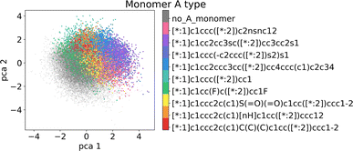 | ||
| Fig. 6 Visualization of the two first principal components of the latent space of the training data. Coloring by A monomer type reveals organization according to the monomer chemistry. | ||
![[thin space (1/6-em)]](https://www.rsc.org/images/entities/char_2009.gif) :
:![[thin space (1/6-em)]](https://www.rsc.org/images/entities/char_2009.gif) 1 to either 1
1 to either 1![[thin space (1/6-em)]](https://www.rsc.org/images/entities/char_2009.gif) :
:![[thin space (1/6-em)]](https://www.rsc.org/images/entities/char_2009.gif) 3 or 3
3 or 3![[thin space (1/6-em)]](https://www.rsc.org/images/entities/char_2009.gif) :
:![[thin space (1/6-em)]](https://www.rsc.org/images/entities/char_2009.gif) 1 would significantly alter the nature of the polymer and thus should not be modified in the immediate neighborhood. For the chain architecture, the impact is slightly less pronounced, but changing from an alternating to a block structure would still substantially alter the polymer's nature.
1 would significantly alter the nature of the polymer and thus should not be modified in the immediate neighborhood. For the chain architecture, the impact is slightly less pronounced, but changing from an alternating to a block structure would still substantially alter the polymer's nature.
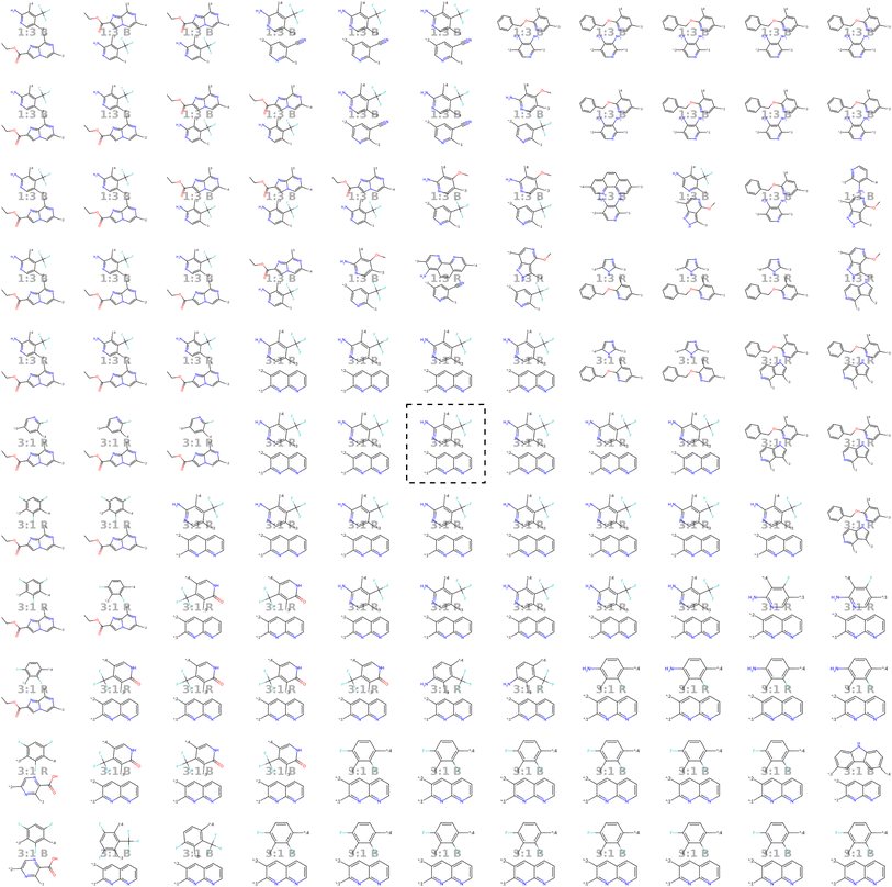 | ||
| Fig. 8 Visualization of the molecular neighborhood using two orthogonal vectors in latent space as proposed by Kusner et al.57. Moving around the random seed polymer in black dashed lines in the center, we can observe step-wise changes in monomer A (bottom one), monomer B (top one), stoichiometry and chain architecture (B: Block, R: Random, A: Alternating). | ||
3.3 Hyperparameter selection
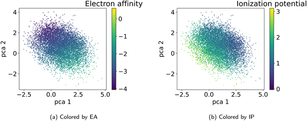
As detailed in Section 2.4, to select the best model we conducted a hyperparameter search over the weights β and α in the loss terms in eqn (2) and evaluated the model using the performance metrics from Table 1. We observed that lower values of β and α enhance reconstruction accuracy by prioritizing the reconstruction term in the loss function. However, achieving high novelty and validity in randomly generated samples requires larger β values. If β is too small, the latent space becomes discontinuous with “holes” or regions of low confidence, leading to invalid polymers when sampled. We found that for this dataset, β values between 0.0003 and 0.0004 work best to optimize the trade-off between reconstruction, validity and novelty. Additionally, we found that a well-structured latent space (LS) is crucial for successful inverse design using optimization algorithms. Ideally, the LS should organize polymers by their properties, as demonstrated in Section 3.2.1. Increasing the weighting factor α improved the organization of polymers regarding their properties, which was visually confirmed by examining PCA plots of the latent space showing clear property gradients (Fig. 7). A sufficiently high α also leads to accurate property predictions, as verified in Appendix B.1.3. Contrary, increasing α too much harms the reconstruction performance. As a result, we select the best model (α = 0.2 and β = 0.0004) according to both the quantitative metrics and visual inspection of gradients in the latent space. In the subsequent section, we use this model for the inverse design approach. Note, that the hyperparameter tuning does not guarantee reaching a globally optimal configuration for the inverse design problem and may vary for new datasets.3.4 Inverse design of novel polymer photocatalysts for hydrogen production
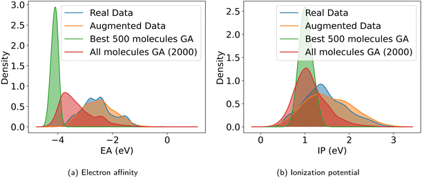
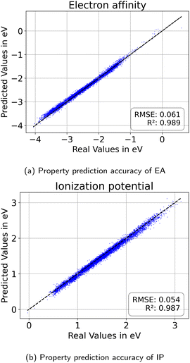
With the objective function defined in eqn (4), we can directly apply optimization techniques to decode novel polymer photocatalysts that best align with our targets. We compare Bayesian optimization (BO) and genetic algorithms (GA), as explained in Section 2.5. For a fair comparison, we report the results for a fixed oracle budget of 2000 generated polymers, and average the results over five runs per optimization algorithm. Furthermore, in Appendix B.1.6 we compare the two algorithms for a fixed run time of two hours. Table 2 shows a comparison of the best objective values of polymers in the training dataset with the decoded polymers using BO and GA. Notably, both BO and GA produce top 3 candidates that better satisfy the objective than the best candidate from the dataset. Inspecting the average objective of the top 10 polymers in Table 2 shows that both optimization strategies outperform selecting the ten best candidates from the dataset, while we observe that the GA outperforms the BO. We conclude that with the aim to obtain a large variety of good candidate polymers, the GA, in combination with our model, is the most effective approach for inverse design in this case study. The result is a library of polymer structures that adhere to the specified target objectives. Fig. 11a and b show the effective distribution shift towards polymers with targeted EA and IP, compared to the wide distribution of properties in the training data. Note that, despite the high property prediction performance on the test set (see Fig. 14a and b), validation through e.g. DFT calculations should be conducted before synthesis. This is increasingly important when specifying open-ended objectives (e.g., minimizing the EA) or when working with objective values outside of the training data distribution, given the lower reliability of property predictions when extrapolating beyond that distribution.| Data | f(z) (top 3) | f(z) (top 10 avg.) |
|---|---|---|
| Training data | −4.027, −4.009, −3.936 | −3.9362 |
| Generated (BO) | −4.194, −4.144,-4.088 | −3.9403 |
| Generated (GA) | −4.224, −4.063, −4.053 | −4.0088 |
As mentioned by Bai et al.,49 even optimal values of IP and EA according to the objective function do not guarantee high HERs. Note that it is important to consider additional factors (beyond electronic properties) that influence the HER for experimental validation. However, the set of candidates after the optimization likely comprises more high-performing materials than a broader set of structures and is thus very valuable for material development. Furthermore, researchers using these methods should carefully consider the importance of different properties (weights in objective function). In our setting with equal weights for both objectives, we observe that the optimization favors low EA values while sacrificing larger deviations of IP from 1 eV.
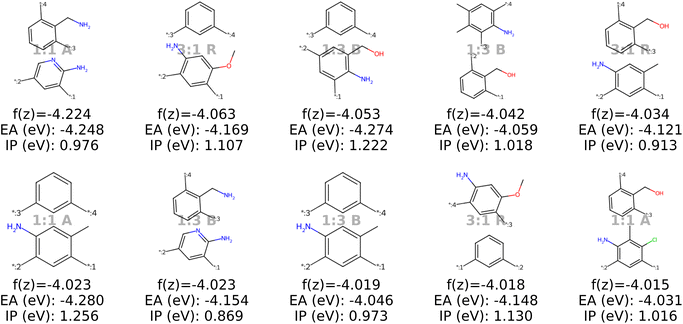 | ||
| Fig. 9 The top ten decoded candidates out of 2000 generated polymers after optimization of the objective function in eqn (4) in latent space using a genetic algorithm. The copolymers are described by monomer A (bottom), monomer B (top), stoichiometry and chain architecture (B: Block, R: Random, A: Alternating). | ||
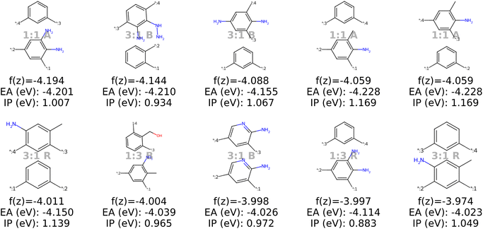 | ||
| Fig. 10 The top ten decoded candidates out of 2000 generated polymers using optimization of the objective function in eqn (4) in latent space using Bayesian optimization. The copolymers are described by monomer A (bottom), monomer B (top), stoichiometry and chain architecture (B: Block, R: Random, A: Alternating). | ||
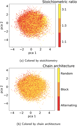
Stoichiometry and chain architecture play a less significant role. For instance, candidates six and ten after BO consist of the same monomers and random chain architecture and have very similar properties, despite the different stoichiometry. Similarly, candidates 1 and 9 differ in stoichiometry and chain architecture, but still possess fairly similar properties. The importance of monomer chemistry compared to stoichiometry and chain architecture aligns with our observations of the latent space structure (Fig. 6 and 13) and the analysis in prior studies.37 Nonetheless, it's important to acknowledge that for other datasets or properties, stoichiometry and chain architecture might play a more critical role in the optimization process.
3.5 Limitations and future work
Polymer properties are influenced not only by the repeat unit chemistry, but also by their higher-order structure and processing conditions. While our work incorporates stochasticity, stoichiometry of monomers and chain architectures, further factors such as average chain length, weight distribution, linking structure, and processing conditions, also play crucial roles. We see the inclusion of hierarchical information in datasets and in informative representations as one of the main challenges of polymer informatics. We expect that this influences the design of future ML model architectures as well as the granularity of predictions.While the dataset we use enables exploration of novel polymer photocatalysts, our results also reveal the need for greater dataset diversity in monomer chemistries and higher-order structural information (stoichiometry and chain architecture). Expanding dataset diversity across all structural levels will help prevent overfitting to monomers or e.g., a set of stoichiometries, and therefore constructing a truly continuous polymer latent space. Specifically, when training on datasets with a larger variety of stoichiometries and monomer connection probabilities (chain architectures), the model architecture (i.e. tokenization) would enable the generation of unseen stoichiometric ratios or connection probabilities. This would naturally increase the novelty and diversity of the generated structures.
Synthesizability is another critical consideration in polymer design, yet existing metrics like the synthetic accessibility (SA) score typically encountered in small molecule discovery are limited in their application to polymers. Polymers possess a hierarchical structure beyond the monomer and their synthesis involves complex steps. Hence, developing a tailored metric that considers polymerization methods, monomer reactivity, and monomer availability is essential for translating computational predictions into experimentally realizable materials.
Lastly, while VAEs are effective at generating data within the training data distribution, they struggle with creating truly novel, out-of-distribution molecules. Techniques like reinforcement learning or genetic algorithms iteratively modifying the molecular structure (e.g. molecular graph) may be suited for out-of-distribution design but require reliable property predictors or experimental validations. When the generated molecules deviate significantly from the training data, the accuracy of property predictors is likely to diminish, underscoring the importance of robust validation methods.
4 Conclusion
In conclusion, our model explores a novel VAE architecture encoding polymer graphs using a graph neural network and decoding polymer strings with a Transformer. With the consideration of stochasticity of monomer ensembles including their stoichiometry and chain architecture our model represents a significant step forward in the inverse design of synthetic polymers, going beyond the repeat unit structure. We leverage a semi-supervised setup to handle partly labelled data, which is promising for a domain like polymer informatics with limited labelled data. Our model is designed to work effectively across a wide range of polymer datasets that consider the same structural levels. Additionally, we consider it to be easily adaptable, making it a useful starting point for further development as new datasets with more complex structural information emerge.Finally, for the use case of conjugated copolymer-photocatalysts for hydrogen production, we demonstrate the capability of our model to generate conjugated copolymers with tailored electronic properties. We do this by using optimization in the latent space that encodes monomer combinations including monomer stoichiometries and chain architectures. Notably, the inverse design approach identifies novel copolymers that exhibit properties better than the best properties in the used training dataset. The results hold promise for accelerating the discovery of new high-performing polymer materials considering their hierarchical structure.
Data availability
The data and code can be found openly accessible on https://github.com/Intelligent-molecular-systems/Inverse_copolymer_design.Author contributions
Conceptualization was carried out by J. M. W. and G. V. G. V. was responsible for data curation, formal analysis, investigation, methodology, software development, validation, and visualization. G. V. wrote the original draft of the manuscript. J. M. W. provided supervision and contributed to the review and editing of the manuscript.Conflicts of interest
There are no conflicts to declare.A Appendices
A.1 Additional details on methods
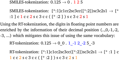
Further the decimal tokenization could be used in future work together with numerical encodings as demonstrated in by Born and Manica.41
 | (6) |
 with minimization of the regularization term DKL(qϕ(z|x(i))‖p(z)), where the prior p(z) is a normal distribution
  . During training, the negative of the lower bound is minimized, as described by Kingma and Welling.42
As a result of the modified components of the VAE, encoding a graph and decoding a string, the variational lower bound in eqn (6) can be rewritten as
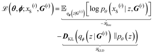 | (7) |
 | (8) |
B.1 Additional results
![[thin space (1/6-em)]](https://www.rsc.org/images/entities/char_2009.gif) :
:![[thin space (1/6-em)]](https://www.rsc.org/images/entities/char_2009.gif) 1 to 1
1 to 1![[thin space (1/6-em)]](https://www.rsc.org/images/entities/char_2009.gif) :
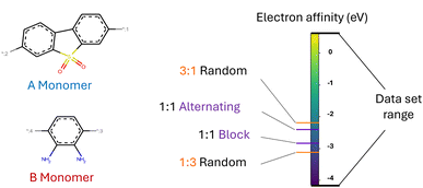
:![[thin space (1/6-em)]](https://www.rsc.org/images/entities/char_2009.gif) 3 leads to a significant drop of the EA compared to the data set range. Further, for a fixed stoichiometry, changing the chain architecture from alternating to block structure leads to a non negligible drop in the EA of the polymer material. This example illustrates that the higher order structure matters to learn accurate structure–property relationships.
3 leads to a significant drop of the EA compared to the data set range. Further, for a fixed stoichiometry, changing the chain architecture from alternating to block structure leads to a non negligible drop in the EA of the polymer material. This example illustrates that the higher order structure matters to learn accurate structure–property relationships.
B.1.4.1 Sampling the neighborhood of high-performing polymer. Sampling around polymers that are known to be high-performing photocatalysts can prove as a powerful approach to generate novel polymers with similarly good or better performance. To do so, we take one high-performing photocatalysts as a starting point and encode the respective graph to a continuous latent vector zseed. Next, we repeatedly add small noise (drawn from
 ) to obtain new latent vectors. We can then decode these new latent vectors to structures. Fig. 15 shows the results of sampling around the polymer with the best experimental HER in Bai et al.49's study, highlighted in black dashed lines. The novel polymers we obtained by sampling around the latent vector of the encoded seed polymer possess a variety of changes from the encoded polymer, where monomer B is varied most. We see that monomer A is altered less, attributable to the limited monomer A variety in the dataset. Same holds for the stoichiometry while the chain architecture is varied more than stoichiometry, meaning that it has less strong signal in the latent space than the stoichiometry (less robust to changes in the latent vector).
 | ||
| Fig. 15 Sampling around the best experimental photocatalyst found by Bai et al.49 The best photocatalyst is first encoded to the latent space. By adding small bits of random noise to the latent representation, we obtain new latent vectors that can be decoded to novel similar polymer photocatalysts. | ||
B.1.4.2 Interpolation between interesting candidates. The second strategy to sample novel polymers without property optimization is interpolation in the latent space. With the aim to find promising novel photocatalysts we can for instance interpolate between the two best polymers found in the work of Bai et al.49. For this we assume that both polymers possess a 1
![[thin space (1/6-em)]](https://www.rsc.org/images/entities/char_2009.gif) :
:![[thin space (1/6-em)]](https://www.rsc.org/images/entities/char_2009.gif) 1 monomer stoichiometry and alternating chain architecture. However, the two best candidates are structurally very similar: monomer A is the same and monomer B is only slightly different. As a result, the interpolation only leads to one additional candidate that is found on the interpolation path (see Fig. 16). While we expect the polymers to be close in the latent space, we could think of more candidates that lie on the interpolation path.Generally, interpolation is more interesting in scenarios where we want to know the path in the chemical space between two structurally substantially different polymers. For instance, we can interpolate between the best polymer and a random polymer in the dataset, leading to a more interesting path as visualized in Fig. 17.
1 monomer stoichiometry and alternating chain architecture. However, the two best candidates are structurally very similar: monomer A is the same and monomer B is only slightly different. As a result, the interpolation only leads to one additional candidate that is found on the interpolation path (see Fig. 16). While we expect the polymers to be close in the latent space, we could think of more candidates that lie on the interpolation path.Generally, interpolation is more interesting in scenarios where we want to know the path in the chemical space between two structurally substantially different polymers. For instance, we can interpolate between the best polymer and a random polymer in the dataset, leading to a more interesting path as visualized in Fig. 17.
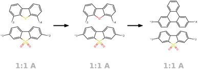 | ||
| Fig. 16 Interpolation in the latent space between the two best copolymer photocatalysts found by Bai et al.49 Starting from the best candidate polymer on the left, we observe only one polymer on the interpolation path to the second best candidate. | ||
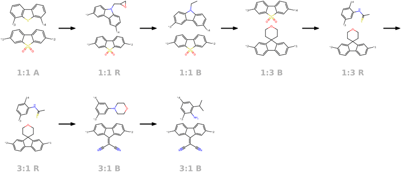 | ||
| Fig. 17 Interpolation in the latent space between the best copolymer photocatalysts found by Bai et al.49 and one random polymer. We observe a step-wise change from on the monomer but level but also on the higher order structural levels, i.e. the monomer stoichiometry and chain architecture. | ||
B.1.5.1 Target electronic properties of a known high-performing photocatalyst. Let us consider the best-performing polymer in Bai et al.49's study which has an EA of approximately −2.64 eV and an IP of 1.61 eV (as reported in the used training dataset37). These values differ markedly from the targets in the objective function in Section 3.4, which aimed for minimal EAs (converging to around −4 eV) and an IP of 1 eV. Hence, we observe that the results in Fig. 18 differ significantly from those in Fig. 9. Comparing the results to the structure of the best molecule, as shown in black dashed lines in Fig. 15, we observe several candidates that are structurally very similar. We also see a variety of structures that satisfy the objective function well but differ structurally from the best polymer reported in the literature.
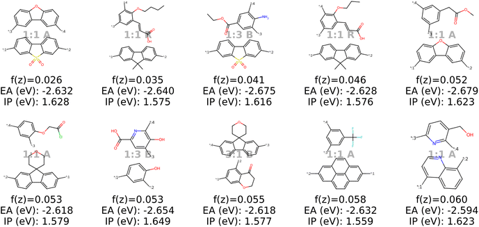 | ||
| Fig. 18 Results when minimizing the objective function using a genetic algorithm (with 2000 oracle calls). This is the modified objective function with EA and IP targeting the values of the best experimental polymer (see polymer in black dashed lines in Fig. 15). | ||
B.1.5.2 Change of target values according to dataset statistics. Second, we adjust the target for IP and EA to the value that exhibits the largest number of well-performing (threshold defined by Bai et al.49) photocatalysts from their experimental validation. As a result, we specify an EA of −2 eV and IP of 1.2 eV as optimal. Also for this modified objective function we observe a different region of the polymer space to be optimal (Fig. 19) compared to the results in Section 3.4.
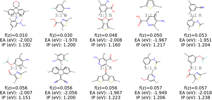 | ||
| Fig. 19 Results when minimizing the objective function using a genetic algorithm (with 2000 oracle calls). This is the modified objective function targeting an EA of −2 eV and an IP of 1.2 eV. The objective matches the property values where most well-performing materials were found according to Bai et al.49 | ||
An interesting detail for both of these experiments is, that the genetic algorithm (GA) converges faster for these two objective functions compared to the objective function in eqn (4) and experiment in Section 3.4. This suggests that specifying property values as target is a simpler task than the open-ended minimization of EA. This could also be due to EAs < −4 being slightly outside of the distribution of the dataset.
| Data | f(z) (top 3) | f(z) (top 10 avg.) |
|---|---|---|
| Training data | −4.027, −4.009, −3.936 | −3.9362 |
| Generated (BO) | −4.159, −4.059, −4.040 | −3.7823 |
| Generated (GA) | −4.467, −4.406, −4.404 | −4.1689 |
The increased computational efficiency of the GA compared to BO, which includes fitting a Gaussian process after each generated polymer, allows the GA to evaluate a significantly larger number of polymers (average over five runs: 8195) than the BO (average over five runs: 930) within the same runtime. Most likely, this also enables the GA to identify more candidates with high objective values. Thus, we conclude that also in this scenario the GA, in combination with our model, is the most effective approach for finding a variety of good candidate polymers.
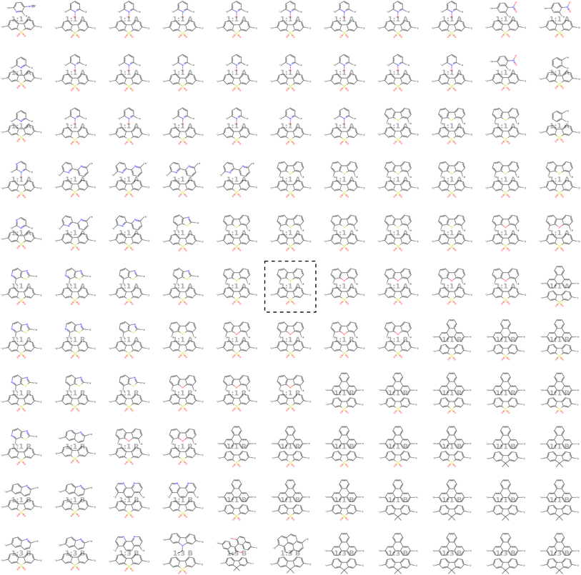 | ||
| Fig. 20 Visualization of the molecular neighborhood (as proposed by Kusner et al.57) of the best performing polymer found by Bai et al.49. Moving around the encoded polymer in black dashed lines in the center, we can observe step-wise changes in monomer A (bottom one), monomer B (top one), stoichioemtry and chain architecture. | ||
References
- S. Mangaraj, A. Yadav, L. M. Bal, S. Dash and N. K. Mahanti, J. Packag. Technol. Res., 2019, 3, 77–96 CrossRef.
- D. S. Morais, R. M. Guedes and M. A. Lopes, Materials, 2016, 9, 498 CrossRef PubMed.
- C. Liu, K. Wang, X. Gong and A. J. Heeger, Chem. Soc. Rev., 2016, 45, 4825–4846 RSC.
- M. F. Maitz, Biosurf. Biotribol., 2015, 1, 161–176 CrossRef.
- C. Yan and G. Li, Adv. Intell. Syst., 2023, 5, 2200243 CrossRef.
- K. Hatakeyama-Sato, Polym. J., 2023, 55, 117–131 CrossRef.
- A. Lavecchia, Drug discovery today, 2015, 20, 318–331 CrossRef PubMed.
- B. Sanchez-Lengeling and A. Aspuru-Guzik, Science, 2018, 361, 360–365 CrossRef.
- C. Bilodeau, W. Jin, T. Jaakkola, R. Barzilay and K. F. Jensen, Wiley Interdiscip. Rev.: Comput. Mol. Sci., 2022, 12, e1608 Search PubMed.
- Y. Du, A. R. Jamasb, J. Guo, T. Fu, C. Harris, Y. Wang, C. Duan, P. Liò, P. Schwaller and T. L. Blundell, Nat. Mach. Intell., 2024, 1–16 Search PubMed.
- A. Lavecchia and C. Di Giovanni, Curr. Med. Chem., 2013, 20, 2839–2860 CrossRef.
- R. Gómez-Bombarelli, J. Aguilera-Iparraguirre, T. D. Hirzel, D. Duvenaud, D. Maclaurin, M. A. Blood-Forsythe, H. S. Chae, M. Einzinger, D.-G. Ha and T. Wu, et al. , Nat. Mater., 2016, 15, 1120–1127 CrossRef PubMed.
- K. Sattari, Y. Xie and J. Lin, Soft Matter, 2021, 17, 7607–7622 RSC.
- X. Zhu, Y. Zhou and D. Yan, J. Polym. Sci. B Polym. Phys., 2011, 49, 1277–1286 CrossRef.
- A. Hult, M. Johansson and E. Malmström, Branched Polymers II, 1999, pp. 1–34 Search PubMed.
- N. Hadjichristidis, M. Pitsikalis, S. Pispas and H. Iatrou, Chem. Rev., 2001, 101, 3747–3792 CrossRef PubMed.
- G. C. Bazan and R. R. Schrock, Macromolecules, 1991, 24, 817–823 CrossRef.
- C. Kuenneth, A. C. Rajan, H. Tran, L. Chen, C. Kim and R. Ramprasad, Patterns, 2021, 2(4), 100238 CrossRef PubMed.
- C. Kuenneth, J. Lalonde, B. L. Marrone, C. N. Iverson, R. Ramprasad and G. Pilania, Commun. Mater., 2022, 3, 96 CrossRef.
- H. Doan Tran, C. Kim, L. Chen, A. Chandrasekaran, R. Batra, S. Venkatram, D. Kamal, J. P. Lightstone, R. Gurnani and P. Shetty, et al. , J. Appl. Phys., 2020, 128(17), 171104 CrossRef.
- G. Pilania, C. N. Iverson, T. Lookman and B. L. Marrone, J. Chem. Inf. Model., 2019, 59, 5013–5025 CrossRef.
- R. Bhowmik, S. Sihn, R. Pachter and J. P. Vernon, Polymer, 2021, 220, 123558 CrossRef.
- R. Ma and T. Luo, J. Chem. Inf. Model., 2020, 60, 4684–4690 CrossRef.
- C. Kim, A. Chandrasekaran, T. D. Huan, D. Das and R. Ramprasad, J. Phys. Chem. C, 2018, 122, 17575–17585 CrossRef.
- C. Kuenneth and R. Ramprasad, Nat. Commun., 2023, 14, 4099 CrossRef CAS.
- C. Xu, Y. Wang and A. Barati Farimani, npj Comput. Mater., 2023, 9, 64 CrossRef.
- R. Batra, H. Dai, T. D. Huan, L. Chen, C. Kim, W. R. Gutekunst, L. Song and R. Ramprasad, Chem. Mater., 2020, 32, 10489–10500 CrossRef.
- M. Ohno, Y. Hayashi, Q. Zhang, Y. Kaneko and R. Yoshida, J. Chem. Inf. Model., 2023, 63, 5539–5548 CrossRef PubMed.
- S. Kim, C. M. Schroeder and N. E. Jackson, ACS Polym. Au, 2023, 3(4), 318–330 CrossRef.
- T.-S. Lin, C. W. Coley, H. Mochigase, H. K. Beech, W. Wang, Z. Wang, E. Woods, S. L. Craig, J. A. Johnson and J. A. Kalow, et al. , ACS Cent. Sci., 2019, 5, 1523–1531 CrossRef.
- L. Schneider, D. Walsh, B. Olsen and J. de Pablo, Digital Discovery, 2024, 3, 51–61 RSC.
- J. Park, Y. Shim, F. Lee, A. Rammohan, S. Goyal, M. Shim, C. Jeong and D. S. Kim, ACS Polym. Au, 2022, 2, 213–222 CrossRef PubMed.
- D.-F. Liu, Y.-X. Zhang, W.-Z. Dong, Q.-K. Feng, S.-L. Zhong and Z.-M. Dang, J. Chem. Inf. Model., 2023, 63, 7669–7675 CrossRef.
- M. Guo, W. Shou, L. Makatura, T. Erps, M. Foshey and W. Matusik, Advanced Science, 2022, 9, 2101864 CrossRef.
- E. R. Antoniuk, P. Li, B. Kailkhura and A. M. Hiszpanski, J. Chem. Inf. Model., 2022, 62, 5435–5445 CrossRef.
- R. Gurnani, C. Kuenneth, A. Toland and R. Ramprasad, Chem. Mater., 2023, 35, 1560–1567 CrossRef CAS PubMed.
- M. Aldeghi and C. W. Coley, Chem. Sci., 2022, 13, 10486–10498 RSC.
- G. Vogel, P. Sortino and J. M. Weber, AI for Accelerated Materials Design - NeurIPS 2023 Workshop, 2023 Search PubMed.
- R.-R. Griffiths and J. M. Hernández-Lobato, Chem. Sci., 2020, 11, 577–586 RSC.
- T. Sousa, J. Correia, V. Pereira and M. Rocha, Applications of Evolutionary Computation: 24th International Conference, EvoApplications 2021, Held as Part of EvoStar 2021, Virtual Event, April 7–9, 2021, Proceedings, 2021, 24, 81–96 Search PubMed.
- J. Born and M. Manica, arXiv, 2022, preprint, arXiv:2202.01338, DOI:10.48550/arXiv.2202.01338.
- D. P. Kingma and M. Welling, arXiv, 2013, preprint, arXiv:1312.6114, DOI:10.48550/arXiv.1312.6114.
- O. Dollar, N. Joshi, J. Pfaendtner and D. A. Beck, J. Phys. Chem. A, 2023, 127(37), 7844–7852 CrossRef CAS PubMed.
- A. T. Müller, K. Atz, M. Reutlinger and N. Zorn, ICML’24 Workshop ML for Life and Material Science: From Theory to Industry Applications, 2024 Search PubMed.
- A. Vaswani, N. Shazeer, N. Parmar, J. Uszkoreit, L. Jones, A. N. Gomez, Ł. Kaiser and I. Polosukhin, Advances in neural information processing systems, 2017, vol. 30 Search PubMed.
- L. Fang, T. Zeng, C. Liu, L. Bo, W. Dong and C. Chen, arXiv, 2021, preprint, arXiv:2101.00828, DOI:10.48550/arXiv.2101.00828.
- C. Li, X. Gao, Y. Li, B. Peng, X. Li, Y. Zhang and J. Gao, arXiv, 2020, preprint, arXiv:2004.04092, DOI:10.48550/arXiv.2004.04092.
- R. Gómez-Bombarelli, J. N. Wei, D. Duvenaud, J. M. Hernández-Lobato, B. Sánchez-Lengeling, D. Sheberla, J. Aguilera-Iparraguirre, T. D. Hirzel, R. P. Adams and A. Aspuru-Guzik, ACS Cent. Sci., 2018, 4, 268–276 CrossRef PubMed.
- Y. Bai, L. Wilbraham, B. J. Slater, M. A. Zwijnenburg, R. S. Sprick and A. I. Cooper, J. Am. Chem. Soc., 2019, 141, 9063–9071 CrossRef CAS PubMed.
- H. Fu, C. Li, X. Liu, J. Gao, A. Celikyilmaz and L. Carin, arXiv, 2019, preprint, arXiv:1903.10145, DOI:10.48550/arXiv.1903.10145.
- F. Nogueira, Bayesian Optimization: Open source constrained global optimization tool for Python, 2014, https://github.com/bayesian-optimization/BayesianOptimization Search PubMed.
- E. Siivola, A. Paleyes, J. González and A. Vehtari, Appl. AI Lett., 2021, 2, e24 CrossRef.
- N. Maus, H. Jones, J. Moore, M. J. Kusner, J. Bradshaw and J. Gardner, Adv. Neural Inf. Process. Syst., 2022, 35, 34505–34518 Search PubMed.
- A. Tripp, E. Daxberger and J. M. Hernández-Lobato, Adv. Neural Inf. Process. Syst., 2020, 33, 11259–11272 Search PubMed.
- K. Deb, A. Pratap, S. Agarwal and T. Meyarivan, IEEE Trans. Evol. Comput., 2002, 6, 182–197 CrossRef.
- J. Blank and K. Deb, IEEE Access, 2020, 8, 89497–89509 Search PubMed.
- M. J. Kusner, B. Paige and J. M. Hernández-Lobato, International conference on machine learning, 2017, pp. 1945–1954 Search PubMed.
- L. Wilbraham, E. Berardo, L. Turcani, K. E. Jelfs and M. A. Zwijnenburg, J. Chem. Inf. Model., 2018, 58, 2450–2459 CrossRef.
| This journal is © The Royal Society of Chemistry 2025 |

