Techno-economic and environmental impacts assessments of sustainable aviation fuel production from forest residues

Abstract

The aviation sector contributes approximately 2.5% to global GHG emissions, driving a growing interest in mitigating its environmental impacts through use of sustainable aviation fuel (SAF). A critical component in SAF development lies in securing sustainable feedstock supplies to ensure competitive pricing and minimal environmental impact. This novel study compares the techno-economic and life-cycle environmental impacts from cradle-to-gate of SAF production from forest residues as a lignocellulosic biomass feedstock. The fuel production pathway considered in this study includes conversion of lignocellulosic biomass (forest residues) to renewable jet fuel through gasification, producing synthesis gas and subsequently SAF (FT-SPK-SAF) through Fischer–Tropsch synthesis in the presence of a catalyst. Techno-economic models of feedstock (forest residues) supply, pretreatment, and conversion processes for SAF production at 90 Mg per day capacity were developed and evaluated. Considering the value of co-products, the minimum selling price (MSP) of FT-SPK-SAF was $1.87 per kg or $1.44 L ($5.45 per gallon). The global warming impact of forest residue-based SAF was estimated to be 24.6 g_{CO2 eq.} per MJ of SAF, which was lower than that of SAF from other lignocellulosic feedstock types. Additionally, this study evaluated the changes in carbon removal efficiency of SAF when accounting for soil carbon change. The outcomes of this study are useful for developing strategies to achieve economic feasibility and greenhouse gas reduction goals of SAF production from biobased sources, while also outlining performance targets for enhancing its environmental sustainability at a commercial scale.

---

1. Introduction

About 2.5% of the world's greenhouse gas (GHG) emissions related to energy use come from the aviation sector.^1–3 Notably, the aviation transportation emissions have been increasing at a faster rate in recent years compared to those of other transportation modes, e.g., rail, road, or shipping.^4,5 In addition, non-CO₂ GHG emissions from aviation are responsible for a 3.5% increase in the global mean temperature.^6,7 Aviation's non-GHG emissions, particularly NO_x and particulate matter, also have effects on local air quality, impacting human health. Although aviation's emissions might appear small compared to other sectors, their rapid growth significantly impacts climate change, exacerbated by technical and operational challenges that hinder GHG reduction efforts in this industry.^6,8 To meet the net zero emissions goal set by the Paris Agreement in 2050, all industries need to make major changes, particularly aviation. Aviation faces unique challenges due to its complexity and high energy consumption. While the transportation sector is largely shifting towards renewable energy, predominantly through the electrification of vehicles, this approach proves unfeasible for aviation due to safety concerns, limited energy density, infrastructure constraints for charging, battery weight, and flight range limitations.^9–12 To achieve the net-zero emissions scenario outlined in announced policy pledges, the International Energy Agency (IEA) estimates that SAF must comprise over 15% of aviation fuel demand by 2030.¹³

SAF can be produced from several biobased feedstocks, including lignocellulosic biomass such as forest residues and corn stover, starch-based feedstocks such as corn grain, and oilseeds such as canola, camelina, soybean, and pennycress.^14–18 Lignocellulosic biomass, derived from plants, is primarily composed of cellulose, hemicellulose, and lignin. It can be categorized into types such as agricultural residues (e.g., corn grain and oil seeds), forestry residues (e.g., wood chips and sawdust), energy crops (e.g., switchgrass and Miscanthus), and industrial wastes (e.g., paper mill sludge). Each type varies in composition and requires specific pretreatment and conversion processes to efficiently produce biofuels and bioproducts. However, producing SAF from most of these feedstocks at a commercial scale is still challenging due to high production costs, competition with food resources, land use changes affecting ecosystems, and environmental impacts from feedstock production and conversion processes.^16,19–22

The advantages of SAF production technologies depend on the availability of appropriate feedstocks such as forest and agricultural waste, used cooking oil, CO₂ captured from the air, and green hydrogen.²³ Converting these low-carbon and abundant feedstocks to SAF can achieve sustainable decarbonization.²⁴ Of different feedstocks that are available for the production of SAF such as oils and fats, sugar, municipal waste and forest residues, forest residues are identified as the most abundant feedstock.^25,26 In addition, collection of forest residues for the purpose of SAF production reduces the risk of forest fire and manages pest population by reducing fuel loads.

SAF can be produced from different pathways. Four of the most common technologies include alcohol-to-jet, syngas-to-jet, sugar-to-jet, and oil-to-jet. In alcohol-to-jet, intermediates such as ethanol and butanol, can be converted to jet fuel through dehydration and oligomerization processes.^27–29 Syngas-to-jet technology includes gas fermentation and Fischer–Tropsch synthesis to produce SAF from hydrogen and carbon monoxide.³⁰ The sugar-to-jet technology includes catalytic upgrading or biological conversion processes to produce hydrocarbons from sugars and sugar intermediates.^31,32 The oil-to-jet technology is used for conversion of oil extracted from oleaginous feedstocks, including oilseeds and other oil- or lipid-based feedstocks, such as algae and waste oil, into renewable jet fuel.^18,33 Due to high yield and potential reduction in GHG emissions, conversion of forest residues to SAF through the Fischer–Tropsch process has high potential as discussed in the Annexes of American Society for Testing Materials (ASTM) D7566.³⁴ To ensure that the SAF meets technical specifications for high performance and quality requirements for current aircraft engines and airport fueling infrastructure, ASTM approves SAF blending with conventional jet fuel to be restricted to 50% of maximum when the SAF is produced through specific type of biomass and production pathways.

The net organic carbon change in soil due to biomass production is computed by considering the net difference between carbon captured by crops through photosynthesis and carbon released through respiration and harvest. It reflects the immediate effectiveness of soil carbon sequestration practices in removing carbon from the atmosphere. The net carbon change shows the net difference between carbon entering the soil (from plant residues, dead roots, etc.) and carbon leaving the soil (through decomposition). It also signifies the long-term storage potential of removed carbon from the atmosphere. However, it does not account for the previous cradle-to-grate life cycle assessment (LCA) reports. In this paper, we calculate the net carbon change in soil for forest residue harvest for 100 years and net GHG emissions from SAF production from forest residue feedstock. This net carbon change in soil provides comprehensive understanding of the total carbon removal potential by SAF.

Production of SAF is currently incentivized through a tax credit under the Inflation Reduction Act (IRA) of 2022 in the United States (U.S.), which ranges from $0.33 to $0.46 per liter ($1.25 to $1.75 per gallon), depending on the degree of lifecycle GHG emission reduction achieved.³⁵ Specifically, a SAF production facility that accomplishes a GHG emission reduction of 50% and complies with prevailing wage requirement, qualifies for a tax credit of $0.33 per liter. For SAF that surpasses the 50% GHG emission reduction threshold, an incremental credit of $0.00263 per liter can be claimed for each percentage point reduction in GHG emission beyond 50%, up to a maximum additional credit of $0.1321 per liter.³⁶ Under a different method for incentivizing SAF production, every equivalent gallon of renewable fuels with respect to pure ethanol as the basis is assigned a specific RIN (Renewable Identification Number) at its point of generation or origination.³⁷ D3 RIN credits are also available for biofuels produced using specific cellulosic feedstock from forest. Currently the D3 RIN price is $2.95 or $38.31 per MMBTU or $1.65 per kg of SAF.³⁸ In development towards actual implementation, SAF derived from forest residues has been utilized by several airlines for demonstration basis.^39–43 For example, Japan Airlines has used SAF produced by Velocys using woody biomass residue feedstock. However, for SAF to emerge as a feasible substitute for conventional petroleum-based jet fuel, production of SAF with the current level of resources and technology should be feasible for large-scale production, be economically competitive, and offer environmental advantages.^44–48 In the economic analysis of SAF production, assuming an average credit price of $200 per metric ton of CO₂ eq. for the Low Carbon Fuel Standard (LCFS), the minimum selling price (MSP) of SAF can be adjusted to $1.124 per kilogram.

The minimum selling price (MSP) and lifecycle GHG emissions for Sustainable Aviation Fuel (SAF), specifically Fischer–Tropsch Synthetic Paraffinic Kerosene (FT-SPK) produced from forest residues in the USA, has not been thoroughly explored. Its impact depends on variations due to differences in the production technology, cost and carbon intensity in the feedstocks depending on the location.⁴⁹ Previous studies have used Argonne National Laboratory's LCA tool, GREET (Greenhouse Gases, Regulated Emissions, and Energy Use in Technologies), to calculate GHG emissions from harvesting forest residues for biofuels.⁵⁰ In the GREET model, material and energy requirements for harvesting systems are based on regions like the Southeastern US and Inland West US, which differ in harvesting systems, forest types, and terrain compared to the Northeast US. In those studies, only diesel yield is reported, not jet fuel yield. It is assumed that jet fuel yield is about 25% of the diesel yield.^51,52 This study used SimaPro, an LCA modeling software that provides detailed unit processes and allows for greater flexibility in assessing various scenarios.^53,54 This novel study focuses on FT synthesis for producing SAF (FT-SPK), where SAF yield is higher than diesel yield. We evaluated optimal use of resources for the sustainable production of SAF and assessed both the MSP and the LCA.

The main objective of this study is to evaluate the techno-economics and life-cycle environmental impacts from cradle-to-gate of FT-SPK production from forest residues. The Pacific Northwest states of Washington, northern California, and Oregon were selected as regions of biomass supply and for considering the feedstock supply price for techno-economic analysis (TEA) models.⁵⁵ Process models for SAF production from forest residue feedstocks are developed; and resources and consumables requirements, equipment capacities, labor and utility requirements, costs, revenue, and credits are estimated (ESI†, Table 1). Outcomes of this study involving optimization of the process for TEA, LCA, and its effect on soil carbon are useful for developing policy and decision making frameworks.⁵⁷ It also helps to identify performance targets for improving environmental performance of SAF production from lignocellulosic feedstocks (i.e., forest residues) at a commercial scale.

Table 1 Assumed economic parameters for SAF from forest residues

Economic parameters	Assumed values
Sustainable aviation fuel output (Mg per day)	90
Loan rate	8%
Loan term	10 years
Plant life	25 years + 36 months for construction
Income tax rate	17.2%^56
Inflation	2%
Working capital	20% annual operating costs
Depreciation schedule	10 years, calculation method: straight line^56
Operations days per year	330 (90% uptime)

---

2. Materials and methods

2.1 Techno-economic modeling

2.1.1. System description. The plant capacity considered for this analysis was 90 Mg SAF per day. To produce this amount of SAF, 960 Mg per day biomass feedstock at 30% moisture content is required. This SAF plant capacity is similar to that of the small-scale green diesel plant in the U.S. Initial commercial biobased SAF (Sustainable Aviation Fuel) plant is likely to have a production capacity similar to the plants that currently make green diesel from natural resources.^58–61 The main operations of the gasification-FT (GFT) process include biomass pretreatment (crushing or conditioning of biomass depending on the type of feedstock), gasification of biomass, clean-up of syngas, FT synthesis, upgrading and separation, as well as cogeneration of electricity (Fig. 1). More details of the processes are provided later in the study.

Fig. 1 Overview of the gasification-Fischer–Tropsch process for SAF production from forest residues⁶² (main product process flow in red and byproducts and emission in black).

The process model was developed using SuperPro Designer software version 12.^63,64 The results obtained from the built-in model of SuperPro Designer software were utilized for equipment sizing and determining the required number of different equipment.

2.1.2. Process modeling for gasification-Fischer–Tropsch.
2.1.2.1 Pretreatment. The initial size reduction step reduces the biomass to a dimension of 12 mm, which is then subjected to a drying process. This drying is facilitated by a rotary dryer to achieve a feedstock to moisture ratio of 9 : 1, achieving a final moisture content of 10% on a wet basis.⁶⁵ The gasifier is fed with air and steam. Gasification operating conditions are set at 28 bar and temperature at 871 °C. Diethanolamine (DEA) is used to separate both H₂S and CO₂ from the sour syngas; the sulfur content is reduced to a maximum of 0.2 ppm.
2.1.2.2 FT synthesis. FT synthesis produces a mixture of long-chain hydrocarbons. This study considers low-temperature FT as the products under these conditions contain a higher amount of kerosene and less severe upgrading the FT product is required.²⁷ The Water Gas Shift (WGS) reaction is carried out at 150 °C and 21 bar to obtain a H₂/CO ratio of 2.37, which has been suggested as the optimum value (Table 3 in the ESI†).⁶⁶ The syngas temperature is increased to 200 °C in the FT reactor, where a cobalt-based catalyst is used.^28,67 We selected a cobalt catalyst for the FT reaction and Cu–ZnO–Al₂O₃ for the WGS reaction in our process model because they are commonly used catalysts in Fischer–Tropsch synthesis due to their high activity and selectivity for producing long-chain hydrocarbons, which are desirable for producing jet fuel. The FT scheme, described in the ESI†, converts the syngas into fuel fractions. The gas and liquid fractions are then separated, followed by the aqueous phase removal from the liquid hydrocarbons.
2.1.2.3 Refining: hydrocracking. The mixture of gases and liquid hydrocarbons leaving the FT reactor is separated for further processing, which can involve decrease in temperature (to 40 °C) and gas liquid separation using difference in densities. We used the 0.5Pt/Y(100)35A catalyst for the hydrocracking reaction in our process model as it showed high catalytic activity to obtain sustainable aviation fuel from higher chain hydrocarbons (n-heptadecane (C17)). In the subsequent step, the liquid product is refined to fulfill the required fuel specifications through hydrocracking. Finally, separation is performed by distillation processes as illustrated in Fig. 2 and 1 of the ESI†.

Fig. 2 System boundary for the cradle-to-gate life-cycle assessment of sustainable aviation fuel (SAF) production from forest residues.

For this study, wax is not a desired product and to maximize jet fuel production, a hydrocracking unit is incorporated in the process. The aim of the hydrocracker is to break down long hydrocarbon chains to obtain smaller hydrocarbons and to reduce the concentration of unsaturated hydrocarbons in the product since the unsaturated compounds can cause gum formation which is not desired for jet fuel. Operating conditions, such as temperature, pressure and H₂ inlet flow, affect the severity of the hydrocracking reactions and therefore, the product distribution. Following the research by Teles et al., 50 bar pressure, 277 °C temperature, and 1.5% hydrogen were chosen for mild hydrocracking that produces middle distillates (Table 3 in ESI†).⁶⁸

2.1.2.4 Refining: separation. In the separation process two distillation columns were used to separated flue gases and green diesel separately. Liquid products from the hydrocracking are sent to the decanter, where the aqueous fraction of the liquid mixture is separated at the bottom. The mixture of C_8–16 separates at the top and further was used in the distillation column. Flue gases were separated from first distillation column (2 m diameter and 14 stages) at 125 °C. In the next step, SAF and green diesel were separated in the second distillation column (2 m diameter and 15 stages) operated at 210 °C. In this analysis, the mass yield for SAF was 9.4%, with approximately 2% mass yield of green diesel from biomass with moisture.
2.1.2.5 Power generation unit. Electrical power is produced in a gas turbine generator. The fuel gas was obtained primarily from the gasification section, and used in the FT reactor and the upgrading section.⁶⁹ In the gas turbine, the fuel gas phase was combusted with compressed air and then expanded to atmospheric pressure to generate electricity. The N₂ used in gasification exits from this section. The plant is electricity self-sufficient, and so no additional fossil sources are required.

2.1.3. Economic analysis. The total facility construction period and startup period are assumed to be 36 months and 4 months respectively. Purchase prices of equipment items are estimated for their required size using the size from the process model and approach available in the literature.^58,70–73 In particular, equipment purchase prices are calculated using an exponential scaling factor of 0.65 and the year of analysis (eqn (1)).^58,70,71

Cost of equipment = base cost × (study size/base size)^{scalling factor} (1)

The parameters and assumptions for estimation of the total investment for establishing the forest residue conversion facilities are obtained from the SuperPro Designer model.

Annual operating costs are estimated by including the costs associated with raw materials, labor, utilities, laboratory, and quality control, as well as facility-dependent cost. Facility-dependent cost accounts for the costs associated with the equipment maintenance, depreciation, insurance, taxes as well as other overhead costs.⁶³ Labor work hours are estimated based on the labor needs for different operations or sections in the process. The labor basic rate is considered to be $20 per h,⁷⁴ and the labor cost is estimated using the following eqn (2):⁶³

Labor cost = basic rate × (1 + benefits + supplies + supervision + administration) × labor use (2)

where the benefits, supplies, supervision, and administration factors were assumed as 0.40, 0.10, 0.20 and 0.60, respectively.⁶³

Cost calculations are done considering nth-plant scenarios, assuming that this technology has been commercially proven and multiple industrial plants are up and running successfully.⁷⁵ Techno-economic analysis (TEA) is designed to provide a realistic assessment of project costs by intentionally excluding certain expenses, such as contractor's fees. Such exclusion helps to avoid artificial inflation of project financial burdens, ensuring a more accurate economic evaluation.⁷⁵ Prices of materials used, utilities required, as well as the main product and byproducts of the process are presented in Table 1. The average biomass feedstock cost is considered to be $40 per Mg with 30% moisture content (weight basis) or $57 per ODT^55,76 (price varies from $30 to $82 per ODT in the U.S.).

The CuO–ZnO–Al₂O₃ catalyst is used in the water gas shift reaction and a Pt-supported catalyst is used in the hydrocracker reactor.^45,77,78 The amount of catalyst required is calculated by dividing the syngas mass flow rate with the weight hourly space velocity (WHSV) and it is assumed that the catalyst will be replaced every 3 years (ESI†, Table 2). Excess electricity is assumed to be sold to the electric grid and considered to be a byproduct. The credits associated with the production of byproducts, i.e., electricity, green propane (biogenic) and green diesel are estimated by considering their market prices (Table 2). Capital and operating costs are used to calculate the MSP of SAF at the biorefinery gate.⁷⁵

Table 2 Prices for materials, utilities, main product and co-products of forest residue conversion to sustainable aviation fuel

Item	Units	Price ($ per unit)	References
Bulk material
Biomass	Mg	40	55
Diethanolamine	kg	1	79
Water	m^3	0.0002	75
Catalyst for WGS	kg	5	80
Catalyst for the Fischer–Tropsch process	kg	33	75
Catalyst for hydrocracking	kg	20	81
Utilities
Standard power	kW h	0.081	82
Steam	Mg	12.00	SuperPro built-in model
Steam (high pressure)	Mg	20.00
Cooling water	Mg	0.0001
Chilled water	Mg	0.0010
Coproducts
Green propane	kg	1	83
Green diesel (C17–C22)	kg	1	84

---

2.1.4. Life cycle inventory (LCI) analysis. The elaboration of the LCI for this study is based on the mass and energy balances, resulting from the process modelling in Superpro. This data includes normalized values for the conversion of the main feedstock into jet fuel and secondary products such as green propane, green diesel, and electricity, all measured per 1 MJ of jet fuel.

2.1.5 Life cycle assessment (LCA). The LCA is conducted according to the standardized approach outlined in ISO 14040 (2006) and ISO 14044 (2006) to ensure the consistency and transparency of the LCA studies.⁸⁵ According to this approach, the LCA is composed of four main steps: (1) definition of the goal and scope of the study; (2) inventory analysis; (3) finding the potential environmental impacts; and (4) interpretation of the results. This study seeks to identify most significant environmental input–output flows (i.e., hotspots) in SAF manufacturing based on life-cycle impact assessment (LCIA) results. The LCI flows are converted into environmental impacts using U.S. EPA's (Environmental Protection Agency) Tool for Reduction and Assessment of Chemical and other environmental Impacts (TRACI) version 2.1 impact assessment method⁸⁶ available in SimaPro 9.5 software.^53,86 Different environmental impact categories cannot be directly compared or added because of different measuring units. This study focuses on the following 10 impact categories: (1) global warming (kg CO₂ eq.), (2) ozone depletion (kg CFC-11 eq.), (3) photochemical smog formation (kg O₃ eq.), (4) acidification (kg SO₂ eq.), (5) eutrophication (kg N eq.), (6) carcinogenic (CTUh), (7) non-carcinogenic (CTUh), (8) respiratory effects (PM2.5 eq.), (9) ecotoxicity (CTUe), and (10) fossil fuel depletion (MJ surplus).

2.2.1. Goal and scope definition. The goal of this LCA is to find the environmental performance of the integrated system, which represents a biomass utilization process where the biomass is converted to SAF.

The system boundaries are set such that the LCA analyzes all the processing steps until the final product is produced. The selected functional unit is 1 megajoule (MJ) of SAF while the LHV (Lower Heating Value) of the SAF is considered to be 43 MJ kg⁻¹.⁸⁷ The global warming (GW) impact of technology evaluated in this work is compared with existing SAF production pathways, as well as with regulatory standards, such as the U.S. Renewable Fuel Standard (RFS). RFS sets explicit thresholds for the reduction of CO₂ equivalent (CO₂ eq.) emissions for alternative fuels compared to the conventional jet fuel. In the U.S. the emission from SAF should be below 89 g_{CO2 eq.} per MJ. Synthesized jet fuel would qualify as SAF under RFS if it demonstrates at least a 50% reduction in GHG emissions compared to fossil-derived jet fuel, with a higher threshold of 60% reduction in GHG emission required for fuels to be categorized as a cellulosic biofuel under the D3 RIN category.^88,89 Under European Renewable Energy Directive II (RED II), a 70% reduction in GHG emissions is necessary for compliance compared to 94 g_{CO2 eq.} per MJ.^90,91 In the UK, it is being considered that for SAF to receive credits under their SAF mandate, it will be required to achieve a 70% GHG saving compared to a fossil fuel benchmark of 94 g_{CO2 eq}. per MJ.⁹² In the LCA analysis, the net carbon change in soil is also estimated, although there is currently no regulation for this specific environmental impact.

2.2.1.1 System boundaries for the LCA. The system boundaries for the LCA are more expanded than those of TEA. In LCA, emission of off-gases (combustion gases) from power generation, processing and cooling water use and transportation of forest residues to facilities are also taken into consideration. Fig. 2 and S3† illustrate the stages included in this environmental evaluation.

3. Results and discussion

3.1 Capital cost

The total capital investment for the SAF biorefinery, which uses forest residue input capacity of 960 Mg per day and produces 90 Mg of SAF per day, is estimated to be approximately $422 million (Fig. 3). Total plant direct costs of $296.3 million contribute approximately 70.2% to the total investment for SAF production, while indirect costs of $74.1 million contribute approximately 18%. Costs for equipment purchases, installation, and associated piping are the main contributors to total plant direct costs, accounting for approximately 34%, 27%, and 10%, respectively. The following sections have significant contributions to the overall capital costs: gasification, gas separation, and distillation. The significant contribution of the separation section for the equipment purchase cost is mainly due to the distillation towers needed to separate SAF mentioned in separation section. Most expensive equipment items are found to be high-air separation units and gasifiers mainly due to their high capacities. The results are in line with those of previous studies on SAF production from forest residues.^16,58 In an alternate option to FT gasification, we can use hydrothermal gasification, which operates under different conditions (typically lower temperatures but higher pressures using water as the medium), could potentially influence the efficiency and environmental impacts of the SAF production process. It may offer advantages in terms of higher carbon conversion efficiencies and reduced tar formation, which could lead to different lifecycle greenhouse gas (GHG) emission profiles and overall techno-economic performance compared to traditional gasification methods.⁹³ Indirect costs are mainly attributed to plant engineering. In addition, working capital ($2.3 million) and startup costs ($20 million) collectively contribute approximately 5% to the total investment (Fig. 3).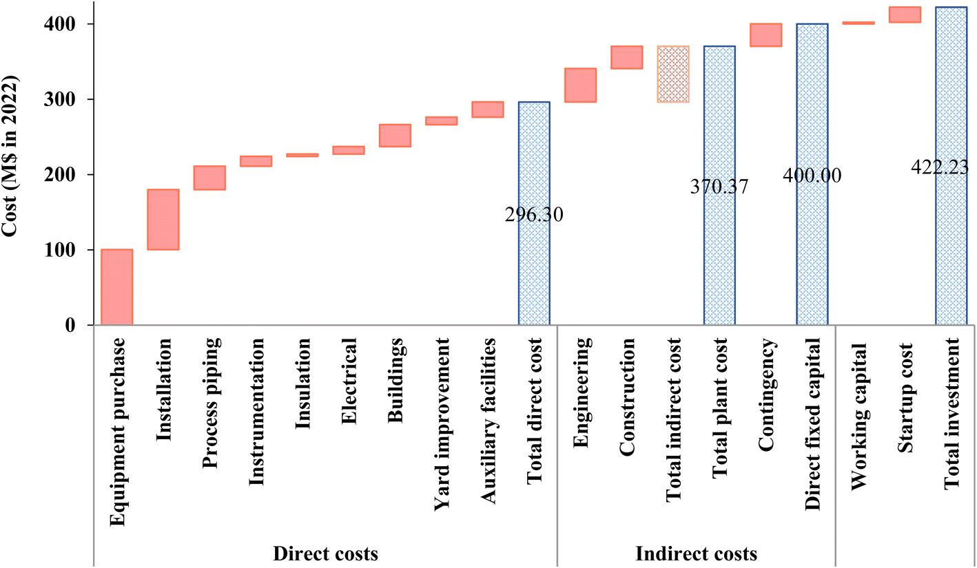

Fig. 3 Capital cost of commercial-scale sustainable aviation fuel production from forest residues; year of analysis 2022.

3.2 Operating cost and MSP

In SAF production from forest residues, the contributions of forest residues, facility, and utility cost to the annual operating cost ($79 million) are estimated to be 16%, 69%, and 8%, respectively (Fig. 4). High utility cost is mainly due to higher amount of high-pressure steam used for heating in pretreatment, FT synthesis and separation of the synthetic crude mixture. The significant labor cost for plant can be attributed to high labor requirement for multiple operation steps such as the gasification reaction, FT synthesis, hydrocracking, gas turbine, and distillation needed for different products, including green propane, green diesel and SAF. The cost of forest residues, $12.6 million, contributes more than 97% to the total material cost.

Fig. 4 (A) Operating cost and (B) minimum selling price of sustainable aviation fuel (SAF) production from forest residues and (C) historical price fluctuation of commercial jet fuel.

The unit production cost of SAF without considering revenue from byproduct production is estimated to be ∼$2.69 per kg (Fig. 4). The unit production cost and MSP of SAF at 0% gross margin after considering revenue from byproducts is $1.87 per kg. The revenue earned by selling excess electricity, green diesel and green propane reduced the unit production cost of SAF by $0.56 per kg $0.24 per kg and $0.015 per kg, respectively.

The cost of commercial jet fuel from fossil resource is $0.87 per kg, lower than that of SAF from biobased feedstocks.⁹⁴ The conversion efficiency of the process from biomass to SAF is 9.4%. In related literature, the feedstock cost has been reported to be the main contributor to the operating cost of similar products, including SAF from camelina⁹⁵ and hydrogenated renewable diesel from canola.⁹⁶ The main reason for the high contribution of forest residues in the production cost was the cost of feedstock supply at refinery required for conversion to SAF at the selected biorefinery capacity. Reduction of the feedstock supply cost can significantly improve the economics of SAF or any other bioenergy products.^97–99 Improving the logistics operations in forest residue supply is one of the factors which can significantly reduce the feedstock price. Other consumables, such as solvent-diethanolamine and catalyst, accounted for approximately 2% of the total material cost.

The main contributors to the total credit were electrical power ($0.56 per kg SAF) and green diesel ($0.24 per kg SAF). The net cost to produce SAF is estimated to be $1.87 per kg, assuming a 0% profit margin. However at 10% IRR,⁷⁵ the MSP of SAF at the biorefinery gate is estimated to be $2.50 per kg, which is in the range of MSP of SAF from similar biobased feedstocks. This result is in line with the results of previous studies on the techno-economics of SAF production from similar biobased feedstocks.^{19,40,100,101} The SAF biorefineries typically generate additional credit from selling coproducts, including LPG, electricity, and green diesel. Thus, any upgrading in the byproduct's values can increase the selling prices and further reduce the MSP of SAF.¹⁰² Evaluating the impacts of variabilities in the prices of byproducts can help identify the key parameters affecting the economics of SAF. Although the cost of green diesel is lower than that of similar SAF, the byproduct credit associated with green diesel is estimated to be less than the byproduct credit associated with SAF (Fig. 5). There are several uncertainties in the cost estimates. For example, if inflation increases up to 4%, it can increase the unit production cost to $1.93 per kg. The cost of forest residues varies widely, ranging from $20 to $80 per tonne. This can cause the SAF production cost to increase from $1.41 per kg to $2.27 per kg.

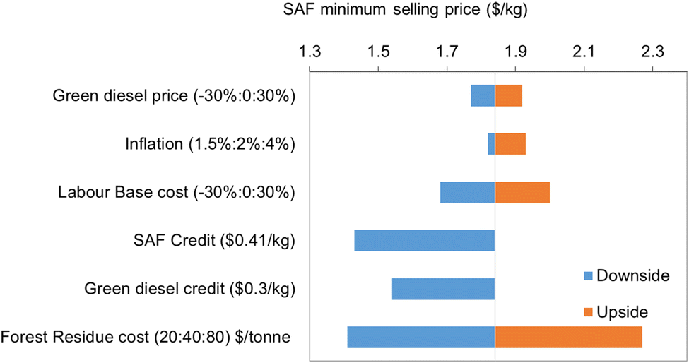Fig. 5 Sensitivity analysis for the SAF MSP from forest residues ($ per kg).

In a comparative analysis, the MSP of SAF from forest residues is competitive with other feedstocks (Fig. S2†). SAF produced from municipal solid waste has an MSP between $0.9 to $2.1 per liter for plant capacity of 100 to 500 million L per year. The MSP of SAF from agricultural residues ranges from $2 to $3.8 per liter from plant capacity of 100 to 300 million L per year. Increase in plant capacities generally benefit from economies of scale, resulting in a lower MSP of SAF from forest residues. Additionally, different production technologies impact costs; the alcohol-to-jet (ATJ) pathway for SAF from agriculture residue has MSPs ranging from $2.2 to $2.5 per liter, which is higher than that of the FT-SPK process but still within the range of lignocellulosic biomass-based SAF production costs ($1.14 to $3.00 per liter).¹⁰³

3.3 Life cycle assesment of SAF

The impact categories assessed, together with the materials used and SAF are shown in Tables 3, 4 and Fig. 6 respectively. These GHG emissions are measured based on a 100-year time horizon (GWP-100) and do not include changes in land use.¹⁰⁴ For the ten impact categories, Fig. 6 shows that the use of steam contributes to the highest environmental impact for most of the impact categories by contributing more than 79% for global warming (GW), 81% of ozone depletion (OD), 41.6% smog, 54.5% respiratory effects (REEF) and 93% fossil fuel depletion (FFD). The use of green propane for production of steam may reduce this impact. The generation of electricity reduces impact in all categories. Regarding the scoring of the impact category values (Table 3), the cradle-to-gate GW impact of producing 1 kg of SAF processes is estimated to be 24.56 g_{CO2 eq.} per MJ or 1.056 kg_{CO2 eq.} per kg. In comparative analysis (Fig. 7), the results of Carbon Offsetting and Reduction Scheme for International Aviation (CORSIA)'s gasification-FT LCA analysis align with those from the GREET model, which estimates direct emissions of 5–12 g_{CO2 eq.} per MJ for FT diesel produced from biomass.¹⁰⁴ In a comparison of sustainable aviation fuels made from biomass sources like switchgrass, soybean oil, palm oil, rapeseed oil, jatropha oil, and algae oil, CO₂ equivalent emissions of it range from 18 to 55 g_CO2 per MJ (Fig. 8).

Table 3 Life cycle environmental impacts for SAF production from forest residues per tonne, cradle-to-gate

Impact category	Units	Total
Ozone depletion	kg CFC-11 eq.	−3.5 × 10^−10
Global warming	kg CO2 eq.	0.02456
Smog	kg O3 eq.	−0.00072
Acidification	kg SO2 eq.	0.00012
Eutrophication	kg N eq.	−0.00012
Carcinogenics	CTUh	−2.1 × 10^−9
Non carcinogenics	CTUh	−6.5 × 10^−9
Respiratory effects	kg PM2.5 eq.	−8.2 × 10^−6
Ecotoxicity	CTUe	−0.11595
Fossil fuel depletion	MJ surplus	0.032769

---

Fig. 6 Cradle-to-gate life-cycle environmental impacts of sustainable aviation fuel (SAF) production from forest residues.

Fig. 7 Comparative global warming impact of SAF from different feedstocks.

Fig. 8 Sensitivity analysis of the global warming impact of SAF production from forest residues.

The nature of different feedstocks changes environmental assessment through amount and type of carbon emission because of different carbon content in feedstocks along with upfront feedstock supply chain efficiencies.^55,105 Gasification of biomass with high carbon content produces more CO₂ compared to those with lower carbon content. Moisture content and ash content of feedstock are other factors impacting the efficiency of the process, and consequently the environmental impacts. The system-wide effect starts with the conventional use of feedstock and impacts environmental assessments. We are using forest residues which do not displace any other product and therefore do not initiate the system wide effect. The effect of use of forest residues compared to pile burning and all decay is discussed in the soil carbon dynamic section.¹⁰⁶

Table 4 Life cycle inventory for Fischer–Tropsch synthetic paraffinic kerosene production from forest residues

	Amount	Units
Output: products
FT_SPK_FR	1	MJ
Output to technosphere: avoided products
Diesel {RoW}| diesel production, petroleum refinery operation | APOS, S	0.006385	kg
Electricity mix eGRIS 2022/US US-EI U	0.1294	kW h
Green propane	0.000467	kg
Inputs from nature
Water, cooling, unspecified natural origin, WECC, US only	18	m^3
Air	2.87	kg
Inputs from technosphere materials/fuel
Proxy_water, at user NREL/US U	0.2239	kg
Diethanolamine {GLO}| market for | APOS, S	0.000232	kg
Forest residues, preprocessed,at conversion facility/ton/RNA	0.2109	kg
Inputs from technosphere electricity/heat
Steam, for chemical processes, at plant/US-US-EI U	0.35	kg
Emission to air
Carbon dioxide, biogenic	0.2941	kg
Carbon monoxide, biogenic	0.0154	kg
Hydrogen sulfide	0.000232	kg
Water	0.247	kg
Oxygen	0.4079	kg
Carbon	0.002103	kg
Hydrogen	0.000935	kg
Methane	0.000701	kg
Nitrogen	2.43	kg
Output to technosphere: waste and emission to treatment
Proxy_disposal, liquid wastes, unspecified to waste water treatment/l NREL/RNA U	0.093	L
Dummy_disposal, wood ash mixture, pure, 0% water, to sanitary landfill/kg/RNA	0.0018	kg
Proxy_disposal, inert solid waste, to inert material landfill NREL/US U	0.041	kg
Proxy_disposal, heavy alkalide naphtha, to sanitary landfill NREL/US U	0.289	kg

---

In GREET model analysis for LCA of SAF, SAF yield is considered to be 20% of green diesel. The increase in yield may increase the GW impact. Regarding the scoring of the impact category values, Fig. 6 shows the overall value for the ten life-cycle environmental impacts. The harmful human ecotoxicity of the FT-SPK-SAF production is negligible. In addition, fossil fuel depletion and acidification are low, reaching only 0.032 MJ surplus and 0.12 g_SO2-eq. per MJ respectively. Impacts on the ozone layer, eutrophication and respiratory effect are not significant.

3.3.1 Uncertainty analysis. Life cycle assessment (LCA) results are critical for informed decision-making, necessitating a rigorous quantification of their uncertainty. To achieve this, we employed a Monte Carlo simulation to examine the impact of data uncertainty on specific impact categories. Each process underwent 1000 simulations, incorporating varied combinations of life cycle inventory (LCI) parameters. Uncertainty was evaluated by analyzing the spread of values relative to their mean. Lower standard errors of the mean indicated more reliable results. Table 5 presents our key findings, including mean values, standard deviations (representing variability), and other relevant metrics. The highest uncertainty was observed in the ozone depletion, ecotoxicity and carcinogenic impact categories. Our analysis indicated that the global warming (GW) impact of SAF ranges from 7.7 to 46.2 g_{CO2 eq.} per kg across the 2.5–97.5% confidence interval. This demonstrates uncertainty for the GW impact and other impact categories considered, affirming the reliability of our dataset. The variations in data selection and inherent data variability do not significantly influence the examined impact categories (Giuliana et al., 2022).¹⁰⁷

Table 5 Uncertainty analysis of life cycle environmental impacts of SAF production from cradle-to-gate^a

Impact category	Units	Mean	Median	SD	CV	2.50%	97.50%	SEM
a Note: SD: standard deviation, CV: coefficient of variation, CV unit is in %. SEM: standard error of the mean (SEM) (standard deviation of the sample distribution of the mean).
Acidification	kg SO2 eq.	1.210 × 10^−4	8.990 × 10^−5	1.330 × 10^−4	1.101 × 10^2	−3.600 × 10^−6	4.810 × 10^−4	4.200 × 10^−6
Carcinogenics	CTUh	−1.900 × 10^−9	−1.000 × 10^−9	4.350 × 10^−9	−2.293 × 10^2	−8.900 × 10^−9	−3.600 × 10^−10	1.380 × 10^−10
Ecotoxicity	CTUe	−1.066 × 10^−1	−7.078 × 10^−2	2.441 × 10^−1	−2.289 × 10^2	−7.870 × 10^−1	2.011 × 10^−1	7.718 × 10^−3
Eutrophication	kg N eq.	−1.200 × 10^−4	−5.000 × 10^−5	2.600 × 10^−4	−2.179 × 10^2	−7.000 × 10^−4	−4.400 × 10^−6	8.210 × 10^−6
Fossil fuel depletion	MJ surplus	3.257 × 10^−2	2.860 × 10^−2	4.309 × 10^−2	1.323 × 10^2	−3.619 × 10^−2	1.318 × 10^−1	1.363 × 10^−3
Global warming	kg CO2 eq.	2.478 × 10^−2	2.406 × 10^−2	9.448 × 10^−3	3.814 × 10^1	7.726 × 10^−3	4.618 × 10^−2	2.990 × 10^−4
Non carcinogenics	CTUh	−5.800 × 10^−9	−4.500 × 10^−9	8.680 × 10^−9	−1.488 × 10^2	−2.800 × 10^−8	5.150 × 10^−9	2.740 × 10^−10
Ozone depletion	kg CFC-11 eq.	−3.700 × 10^−10	−3.800 × 10^−10	1.170 × 10^−10	−3.169 × 10^2	−2.500 × 10^−9	2.140 × 10^−9	3.710 × 10^−11
Respiratory effects	kg PM2.5 eq.	−8.600 × 10^−6	−1.100 × 10^−5	9.350 × 10^−6	−1.085 × 10^2	−2.000 × 10^−5	1.450 × 10^−5	2.960 × 10^−7
Smog	kg O3 eq.	−7.000 × 10^−4	−7.400 × 10^−4	7.910 × 10^−4	−1.137 × 10^2	−2.080 × 10^−3	8.350 × 10^−4	2.500 × 10^−5

---

3.3.2 Cumulative energy demand (LHV). The dataset on sustainable aviation fuel (SAF) production highlights significant cumulative energy demands, particularly in the preprocessing of forest residues and steam generation for chemical processes, which are the largest contributors at about 2.0895 million joules (MJ) (Table S4†). This emphasizes the energy-intensive nature of these stages in SAF production. The analysis shows a substantial reliance on renewable energy sources, especially biomass, which contributes 2.648 MJ. It indicates high significant contribution, however it ensures fewer challenges for sustainable sourcing than fossil fuel-based feedstock.

On the other hand, non-renewable energy sources, including fossil and nuclear, display slightly negative values, suggesting efficient energy recovery or less reliance in certain areas, such as diesel refinement and electricity usage. The slight negative values in other renewable sources like wind, solar, and geothermal, and water-generated energy imply potential net energy losses or lower efficiency in their integration within the SAF production lifecycle. To enhance the sustainability of SAF, it is critical to address these inefficiencies and optimize energy use across all production stages, aiming to boost the efficiency of renewable energy utilization and reduce reliance on non-renewable sources.

3.3.3 Sensitivity analysis. The sensitivity analysis of the global warming (GW) impact for SAF production highlights the significant influence of steam and electricity usage (Fig. 8). When steam usage is increased by 20% to 0.42 kg kg⁻¹, the GW impact increases to 42.7 g_{CO2 eq.} per kg of SAF, whereas a 20% reduction in steam usage decreases the GW impact to 6 g_{CO2 eq.} per kg of SAF. This demonstrates that steam usage had the highest impact on the GW impact of SAF. Similarly, increasing electricity usage by 20% to 0.154 kW h kg results in a GWP impact of 41.9 g_{CO2 eq.} per kg, while a 20% decrease reduces it to 6.89 g_{CO2 eq.} per kg. This indicates that electricity usage also significantly affects the GWP of SAF. Additionally, a decrease in Fischer–Tropsch conversion efficiency to 80% from 100% shows an increase in GWP to 32.7 g_{CO2 eq.} per kg of SAF. Variations in forest residue requirements by ±20% lead to GWP values ranging from 23.8 to 25.3 g_{CO2 eq.} per kg of SAF. Conversely, changes in diethanolamine requirements for gas treatment show a minor impact on GWI, varying from 24.4 to 24.8 g_{CO2 eq.} per kg of SAF. These findings emphasize the critical role of optimizing steam and electricity usage in minimizing the environmental impact of SAF production.

3.4 Soil carbon dynamics

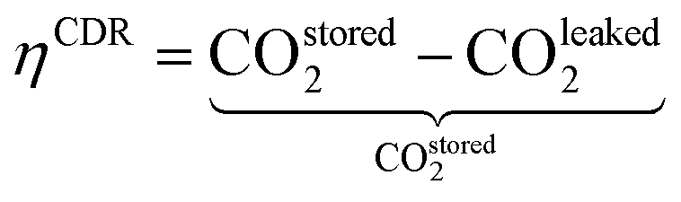
Residue management and soil carbon change have higher impact on carbon removal efficiency in soil.^108–110 Recent studies show that GHG emissions due to a change in soil organic carbon (SOC) over 100 years can contribute to 20 to 65% of increased life cycle GHG emission of gasoline and diesel produced from forest residues.¹¹¹ Optimized methods to handle forest leftovers help to protect soil organic carbon and improve carbon removal in soil from SAF production.¹¹² Alternatively, carbon dioxide can be removed from emission of the FT process. Previous research reported the impact of inclusion of the carbon capture and storage in the FT process using forest residues can reduce the GHG emissions from 15.51 g_{CO2 eq.} per MJ to – 121.83 g_{CO2 eq.} per MJ, however MSP of product SAF increases by about 10%.⁵⁸ Adding carbon capture makes facility increase MSP but forest residue on land management does not make the biofuel more expensive when it is in line with the supply and demand of forest waste.⁵⁸ The SAF combustion is considered for soil carbon removal efficiency.

For analysis of soil carbon dynamics, we evaluate carbon removal from atmosphere in soil due to different forest management practices. A high removal efficiency could be compensated for a slightly lower soil carbon increase, especially if achieved through practices with biofuel production. Here, we define CDR efficiency (eqn (3)), η^CDR, considering the amounts of CO₂ stored and CO₂ leaked over the supply chain:¹¹³

While estimating the amount of CO₂ stored, we take account of carbon uptake by logs, litter residue, litterfall, roots. In CO₂, we take account of forest operations, SAF production, emission from litter and mineral soil. The transportation and combustion of SAF is also considered in this study. Western and Northern States contain the most carbon on the forest floor, and Southern States contain the least. Due to the availability of the soil organic carbon change dataset in the Southern U.S. and results from it will be strong indicator for determination of soil carbon change in the northwest region we used available data for soil carbon dynamics. We calculated carbon removal efficiency of FT-SPK from forest residues with the assumption of use of loblolly pine in the Southern U.S.A.¹¹¹ We use climate scenario of S1 (scenario 1 refers to climate conditions of low temperature and low precipitation at site location of (36.532,−82,210)) and pine growth case of GC1 (pine growth case) for determination of carbon removal following a previous study of Yao et al.¹¹¹

While the 100-year net soil carbon change shows soil carbon change depends on change in the climate, and forest management, it shows the potential of carbon removal from soil. The advantage of carbon removal favors use of forest residues in the production of SAF.

Fig. 9 shows CO₂ removal from the atmosphere through various forest residue management strategies—pile burning (−828.5 Mg_{CO2 eq.} per hectare in 100 years), in situ wood decomposition or all decay (−916.2 Mg_{CO2 eq.} per hectare in 100 years), and biofuel production (−831 Mg_{CO2 eq.} per hectare in 100 years). It shows the potential for forest residues to contribute to climate change mitigation and renewable energy generation. Among these, converting forest residues into (FT-SPK-SAF) biofuel emerges as a compelling climate change mitigation strategy.

Fig. 9 Carbon removal efficiency for forest residue management per hectare over 100 years.

4. Conclusions and prospects

This study evaluates the economic feasibility and life-cycle environmental impacts from cradle-to-gate of producing SAF from forest residues, providing a comprehensive analysis of its environmental and economic advantages. With a GW impact of 1.05 kg_{CO2 eq.} per kg of SAF, the research highlights the significant potential for reducing GHG emissions from the aviation sector. The minimum selling price of SAF is estimated to be about $1.87 per kg, which may further reduce to $1.38 per kg after tax credit from IRA due to ∼72% reduction in GW impact. The key advantage of the SAF production process studied here is a notable reduction in net GHG emissions, indicated by a −831 Mg_{CO2 eq.} per hectare decrease in carbon footprint from fuel production over 100 years. These outcomes suggest that SAF from forest residues not only contributes to lowering the aviation sector's carbon emissions but also presents a cost-effective renewable fuel option.

Future development should aim to optimize the supply chain for forest residues to reduce feedstock costs further and enhance the sustainability of SAF production. This involves investigating strategies to lower transportation costs, improve feedstock yield, and enhance conversion processes. Evaluating the broader social and environmental impacts of SAF production will also support its sustainable integration into the aviation industry. Additionally, exploring high value uses for byproducts and potential policy supports can improve the economic viability of SAF production.

This research offers valuable insights for a broad audience, including academics, industry stakeholders, and policymakers, guiding efforts to commercialize SAF from forest residues. By providing targeted recommendations for future work, this study lays the groundwork for advancing SAF as a sustainable alternative to conventional jet fuels, aligning with global climate goals and supporting the transition to a more sustainable aviation sector.

Data availability

The data supporting the findings of this study are available within the manuscript and its ESI files.† Additional data, including detailed results of the techno-economic analysis and life cycle assessment, are available from the corresponding author upon reasonable request. The soil organic carbon change dataset used in this study was sourced from the recent published research article by Lan et al. Data related to the feedstock cost and economic analyses were obtained from publicly accessible sources and are also available upon request.

Conflicts of interest

There are no conflicts to declare.

Acknowledgements

This work was supported by Agriculture and Food Research Initiative Competitive Grant no. 2020-68012-31881 from the USDA National Institute of Food and Agriculture. The funders had no role in study design, data collection and analysis, decision to publish, or preparation of the manuscript. As some authors of this paper are employees of the USDA FS, the findings and conclusions in this report are those of the author(s) and should not be construed to represent any official USDA or U.S. Government determination or policy. Any use of trade, firm, or product names is for descriptive purposes only and does not imply endorsement by the U.S. government.

References

1. R. Sacchi, V. Becattini, P. Gabrielli, B. Cox, A. Dirnaichner, C. Bauer and M. Mazzotti, Nat. Commun., 2023, 14, 3989.
2. H. Ritchie and M. Roser, Our World in Data, 2024, https://ourworldindata.org/global-aviation-emissions.
3. L. Rye, S. Blakey and C. W. Wilson, Energy Environ. Sci., 2010, 3, 17–27.
4. N. Dolšak and A. Prakash, Clim. Action, 2022, 1, 1–9.
5. Issue Brief|The Growth in Greenhouse Gas Emissions from Commercial Aviation (2019, revised 2022)|White Papers|EESI, https://www.eesi.org/papers/view/fact-sheet-the-growth-in-greenhouse-gas-emissions-from-commercial-aviation,(accessed April 7, 2024.
6. D. S. Lee, M. R. Allen, N. Cumpsty, B. Owen, K. P. Shine and A. Skowron, Environ. Sci.: Atmos., 2023, 3, 1693–1740.
7. H. Ritchie and M. Roser, Our World in Data, 2024, https://ourworldindata.org/global-aviation-emissions.
8. Pathways towards 90% decarbonization of aviation by 2050, Nat. Clim. Change, 2022, vol. 12, pp. 895–896,  DOI:10.1038/s41558-022-01486-3.
9. D. Babuder, Y. Lapko, P. Trucco and R. Taghavi, J. Air Transport. Manag., 2024, 115, 102524.
10. J. Rane, B. Solanki, S. Cary, P. Joshi and S. Ganguly, Overview of Potential Hazards in Electric Aircraft Charging Infrastructure, 2023.
11. Y. Gu, M. Wiedemann, T. Ryley, M. E. Johnson and M. J. Evans, Sustainability, 2023, 15, 15539.
12. Electrifying the production of sustainable aviation fuel: the risks, economics, and environmental benefits of emerging pathways including CO₂ - Energy & Environmental Science (RSC Publishing), https://rsc.66557.net/en/content/articlelanding/2022/ee/d2ee02439j, accessed May 10, 2024.
13. Announced Pledges Scenario (APS) – Global Energy and Climate Model – Analysis, https://www.iea.org/reports/global-energy-and-climate-model/announced-pledges-scenario-aps, accessed February 14, 2024.
14. G. Liu, B. Yan and G. Chen, Renew. Sustain. Energy Rev., 2013, 25, 59–70.
15. C. Gutiérrez-Antonio, F. I. Gómez-Castro, J. A. de Lira-Flores and S. Hernández, Renew. Sustain. Energy Rev., 2017, 79, 709–729.
16. L. Martinez-Valencia, M. Garcia-Perez and M. P. Wolcott, Renew. Sustain. Energy Rev., 2021, 152, 111680.
17. S. H. Mousavi-Avval and A. Shah, Renew. Sustain. Energy Rev., 2021, 149, 111340.
18. S. H. Mousavi-Avval, S. Khanal and A. Shah, Sustainability, 2023, 15, 10589.
19. T. Kandaramath Hari, Z. Yaakob and N. N. Binitha, Renew. Sustain. Energy Rev., 2015, 42, 1234–1244.
20. M. Wang, R. Dewil, K. Maniatis, J. Wheeldon, T. Tan, J. Baeyens and Y. Fang, Prog. Energy Combust. Sci., 2019, 74, 31–49.
21. H. Wei, W. Liu, X. Chen, Q. Yang, J. Li and H. Chen, Fuel, 2019, 254, 115599.
22. S. Searle, N. Pavlenko, A. Kharina, J. Giuntoli, Long-term Aviation Fuel Decarbonization: Progress, Roadblocks, and Policy Opportunities, 2019.
23. Sustainable Aviation Fuel|SAF, https://skynrg.com/sustainable-aviation-fuel/, accessed March 26, 2024.
24. S. Shapiro-Bengtsen, L. Hamelin, L. Bregnbæk, L. Zou and M. Münster, Energy Environ. Sci., 2022, 15, 1950–1966.
25. M. Davis, L. Lambert, R. Jacobson, D. Rossi, C. Brandeis, J. Fried, B. English, et al., Biomass from the Forested Land Base, in 2023 Billion-Ton Report, M. H. Langholtz: TN: Oak Ridge National Laboratory, Oak Ridge, 2024, ch. 4,  DOI:10.23720/BT2023/2316170.
26. M. H. Langholtz, B. J. Stokes and L. M. Eaton, Billion-Ton Report: Advancing Domestic Resources for a Thriving Bioeconomy, EERE Publication and Product Library, Washington, D.C. (United States), 2016.
27. J. Xing, Z. An, Y. Zhang and R. Kurose, Energy Fuels, 2023, 37, 12274–12290.
28. J. Yang, Z. Xin, Q. (Sophia) He, K. Corscadden and H. Niu, Fuel, 2019, 237, 916–936.
29. H.-W. Hsu, Y.-H. Chang and W.-C. Wang, J. Clean. Prod., 2021, 289, 125778.
30. B. H. H. Goh, C. T. Chong, H. C. Ong, T. Seljak, T. Katrašnik, V. Józsa, J.-H. Ng, B. Tian, S. Karmarkar and V. Ashokkumar, Energy Convers. Manage., 2022, 251, 114974.
31. J. Han, L. Tao and M. Wang, Biotechnol. Biofuels, 2017, 10, 21.
32. W.-C. Wang and L. Tao, Renew. Sustain. Energy Rev., 2016, 53, 801–822.
33. W.-C. Wang, L. Tao, J. Markham, Y. Zhang, E. Tan, L. Batan, E. Warner and M. Biddy, Report no.: NREL/TP-5100-66291, National Renewable Energy Laboratory, Denver, CO.
34. Standard Specification for Aviation Turbine Fuel Containing Synthesized Hydrocarbons, https://www.astm.org/d7566-23b.html, accessed February 15, 2024.
35. Sustainable Aviation Fuel Credit|Internal Revenue Service, https://www.irs.gov/credits-deductions/businesses/sustainable-aviation-fuel-credit, accessed July 1, 2024.
36. Alternative Fuels Data Center, https://afdc.energy.gov/laws/13160, accessed April 17, 2024.
37. R. A. Miller, 101 For RINs, https://www.biocycle.net/101-for-rins/, accessed April 17, 2024).
38. AEGIS Hedging, https://instanext.com/insights/lcfs-rin-pricing-report-through-june-23-2023, accessed April 17, 2024.
39. J. Kinder and T. Rahmes, Seattle WA: the Boeing Company, Sustainable Biofuels Research & Technology Program, 2009, p. 16.
40. S. J. Bann, R. Malina, M. D. Staples, P. Suresh, M. Pearlson, W. E. Tyner, J. I. Hileman and S. Barrett, Bioresour. Technol., 2017, 227, 179–187.
41. P. Li, T. E. Yu, C. Trejo-Pech, J. A. Larson, B. C. English and D. N. Lanning, Transport. Res. Rec., 2024, 03611981241230508.
42. M. F. Shahriar and A. Khanal, Fuel, 2022, 325, 124905.
43. K. S. Ng, D. Farooq and A. Yang, Renew. Sustain. Energy Rev., 2021, 150, 111502.
44. G. W. Diederichs, M. Ali Mandegari, S. Farzad and J. F. Görgens, Bioresour. Technol., 2016, 216, 331–339.
45. M. D. Staples, PhD dissertation, Massachusetts Institute of Technology, 2017.
46. E. McGarvey and W. E. Tyner, Biofuels, Bioprod. Biorefin., 2018, 12, 474–484.
47. J. J. Reimer and X. Zheng, Renew. Sustain. Energy Rev., 2017, 77, 945–954.
48. outlook, Velocys technology powers first commercial flight, https://velocys.com/2021/06/21/velocys-technology-powers-first-commercial-flight/, accessed February 16, 2024.
49. J. A. Okolie, D. Awotoye, M. E. Tabat, P. U. Okoye, E. I. Epelle, C. C. Ogbaga, F. Güleç and B. Oboirien, iScience, 2023, 26, 106944.
50. Z. Wang, J. B. Dunn, J. Han and M. Q. Wang, Material and Energy Flows in the Production of Cellulosic Feedstocks for Biofuels for the GREET Model, Argonne National Lab. (ANL), Argonne, IL (United States), 2013.
51. S. de Jong, K. Antonissen, R. Hoefnagels, L. Lonza, M. Wang, A. Faaij and M. Junginger, Biotechnol. Biofuels, 2017, 10, 64.
52. C. H. Geissler, J. Ryu and C. T. Maravelias, Renew. Sustain. Energy Rev., 2024, 192, 114276.
53. Pre Consultants, SimaPro 9.3 Life Cycle Assessment Software Package, 2021, https://simapro.com/wp-content/uploads/2021/12/SimaPro930WhatIsNew.pdf.
54. L. Johnson, B. Lippke and E. Oneil, For. Prod. J., 2012, 62, 258–272.
55. K. Sahoo, E. Bilek, R. Bergman, A. R. Kizha and S. Mani, Biofuels, Bioprod. Biorefin., 2019, 13, 514–534.
56. S. Eswaran, S. Subramaniam, S. Geleynse, K. Brandt, M. Wolcott and X. Zhang, Data Brief, 2021, 39, 107514.
57. K. Morganti, K. Moljord, R. Pearson, M. Vermeire, M. Traver, P. Scorletti, T. de Melo, Y. Wang, P. China, J. Repasky, F. Oliva and A. Bason, Energy Environ. Sci., 2024, 17, 531–568.
58. M. Fernanda Rojas Michaga, S. Michailos, M. Akram, E. Cardozo, K. J. Hughes, D. Ingham and M. Pourkashanian, Energy Convers. Manage., 2022, 255, 115346.
59. R. G. dos Santos and A. C. Alencar, Int. J. Hydrogen Energy, 2020, 45, 18114–18132.
60. H. A. Choudhury, S. Chakma and V. S. Moholkar, in Recent Advances in Thermo-Chemical Conversion of Biomass, Elsevier, 2015, pp. 383–435.
61. H. Gruber, P. Groß, R. Rauch, A. Reichhold, R. Zweiler, C. Aichernig, S. Müller, N. Ataimisch and H. Hofbauer, Biomass Convers. Biorefin., 2021, 11, 2281–2292.
62. G. Diederichs, MSc thesis, Department of Chemical Engineering, Stellenbosch University, 2015.
63. Intelligen, Scotch Plains, New Jersey, available at: https://www.intelligen.com/downloads/SuperPro_ManualForPrinting_v10.pdf, accessed on: 11/27/2019.
64. R. Naveenkumar and G. Baskar, Bioresour. Technol., 2021, 320, 124347.
65. [PDF] Biomass Feedstock and Conversion Supply System Design and Analysis|Semantic Scholar, https://www.semanticscholar.org/paper/Biomass-Feedstock-and-Conversion-Supply-System-and-Jacobson-Roni/019bcedff17a9b8619ace89ef995c27e387e56b8,accessed May 9, 2024.
66. K. Im-orb, L. Simasatitkul and A. Arpornwichanop, Energy, 2016, 94, 483–496.
67. C. Niu, M. Xia, C. Chen, Z. Ma, L. Jia, B. Hou and D. Li, Appl. Catal., A, 2020, 601, 117630.
68. U. M. Teles, F. Fernandes, Chemical and Biochemical Engineering Quarterly, 2014, https://www.osti.gov/biblio/1169237/.
69. H. Jahangiri, A. A. Lappas, M. Ouadi and E. Heracleous, in Handbook of Biofuels Production, ed. R. Luque, C. S. K. Lin, K. Wilson and C. Du, Woodhead Publishing, 2023, 3rd edn, pp. 449–509.
70. S. B. Jones, D. C. Elliott, C. Kinchin, C. Valkenburg, J. E. Holladay, S. Czernik, C. W. Walton, D. J. Stevens, Production of Gasoline and Diesel from Biomass via Fast Pyrolysis, Hydrotreating and Hydrocracking: A Design Case, 2009, https://www.energy.gov/sites/prod/files/2014/04/f14/pyrolysis_report_summary.pdf.
71. Y. Jiang, PhD thesis, West Virginia University Libraries, 2017.
72. N. de Fournas and M. Wei, Energy Convers. Manage., 2022, 257, 115440.
73. S. Wickwire, Biomass Combined Heat and Power Catalog of Technologies, United States Environmental Protection Agency, Washington D.C., 2007.
74. B. Chalermthai, M. T. Ashraf, J.-R. Bastidas-Oyanedel, B. D. Olsen, J. E. Schmidt and H. Taher, Polymers, 2020, 12, 847.
75. D. Humbird, R. Davis, L. Tao, C. Kinchin, D. Hsu, A. Aden, P. Schoen, J. Lukas, B. Olthof, M. Worley, D. Sexton and D. Dudgeon, NREL/TP-5100-47764, National Renewable Energy Laboratory Technical Report, 2011.
76. Intelligen, Inc., https://www.intelligen.com/, accessed November 4, 2023.
77. S. Mitsuoka, K. Murata, T. Hashimoto, N. Chen, Y. Jonoo, S. Kawabe, K. Nakao and A. Ishihara, ACS Omega, 2024, 9, 3669–3674.
78. R. Houston, N. Labbé, D. Hayes, C. S. Daw and N. Abdoulmoumine, React. Chem. Eng., 2019, 4, 1814–1822.
79. I. Alerts, Diethanolamine Prices|Historical and Current, https://www.intratec.us/chemical-markets/diethanolamine-price, accessed April 9, 2024.
80. Cu Zno Al₂O₃ Catalyst-Cu Zno Al₂O₃ Catalyst Manufacturers, Suppliers and Exporters on Alibaba.comCatalyst, https://www.alibaba.com/trade/search?spm=a2700.7735675.the-new-header_fy23_pc_search_bar.keydown__Enter%26tab=all%26SearchText=cu+zno+al2o3+catalyst, accessed April 9, 2024.
81. Pt 1% Pt/al2o3 Platinum On Alumina Cas 7440-06-4 - Buy 7440-06-4,Pt/al2o3,Platinum On Alumina Product on Alibaba.com, https://www.alibaba.com/product-detail/Pt-1-Pt-Al2O3-Platinum-on_1600474831197.html?spm=a2700.galleryofferlist.normal_offer.d_price.208632f11Jd0tk, accessed April 9, 2024.
82. Electric Power Monthly - U.S. Energy Information Administration (EIA), https://www.eia.gov/electricity/monthly/epm_table_grapher.php, accessed April 9, 2024.
83. Weekly U.S. Propane Wholesale/Resale Price (Dollars per Gallon), https://www.eia.gov/dnav/pet/hist/LeafHandler.ashx?n=PET%26s=W_EPLLPA_PWR_NUS_DPG%26f=W, accessed April 9, 2024.
84. J. V. L. Ruatpuia, H. Gopinath, S. Da, H. Sudipta and R. Samuel Lalthazuala, Bioresour. Technol., 2024, 393, 130160.
85. ISO 14040:2006(en), Environmental management — Life cycle assessment — Principles and framework, https://www.iso.org/obp/ui/#iso:std:iso:14040:ed-2:v1:en, accessed May 7, 2024.
86. J. C. Bare, Tool for the Reduction and Assessment of Chemical and Other Environmental Impacts (TRACI), version 2.1 - User's Manual; EPA/600/R-12/554, 2012.
87. M. F. Rojas-Michaga, S. Michailos, E. Cardozo, M. Akram, K. J. Hughes, D. Ingham and M. Pourkashanian, Energy Convers. Manage., 2023, 292, 117427.
88. N. Pavlenko and S. Searle, Assessing the sustainability implications of alternative aviation fuels, 2021, https://theicct.org/publication/assessing-the-sustainability-implications-of-alternative-aviation-fuels/.
89. N. Lange, D. Moosmann, S. Majer, K. Meisel, K. Oehmichen, S. Rauh and D. Thrän, in Progress in Life Cycle Assessment 2021, ed. F. Hesser, I. Kral, G. Obersteiner, S. Hörtenhuber, M. Kühmaier, V. Zeller and L. Schebek, Springer International Publishing, Cham, 2023, pp. 85–101.
90. O. US EPA, Overview for Renewable Fuel Standard, https://www.epa.gov/renewable-fuel-standard-program/overview-renewable-fuel-standard, accessed April 8, 2024.
91. Renewable Energy – Recast to 2030 (RED II) - European Commission, https://joint-research-centre.ec.europa.eu/welcome-jec-website/reference-regulatory-framework/renewable-energy-recast-2030-red-ii_en, accessed April 8, 2024.
92. Aviation fuel plan supports growth of British aviation sector, https://www.gov.uk/government/news/aviation-fuel-plan-supports-growth-of-british-aviation-sector, accessed July 8, 2024.
93. A. Kruse, J. Supercrit. Fluids, 2009, 47, 391–399.
94. Jet Fuel Price Monitor, https://www.iata.org/en/publications/economics/fuel-monitor/, accessed April 12, 2024.
95. X. Li, E. Mupondwa and L. Tabil, Bioresour. Technol., 2018, 249, 196–205.
96. P. Miller and A. Kumar, Sustain. Energy Technol. Assessments, 2014, 6, 105–115.
97. H.-S. Han, A. Jacobson, E. M. Bilek and J. Sessions, Appl. Eng. Agric., 2018, 34(1), 5–10.
98. K. Sahoo, E. Bilek, R. Bergman and S. Mani, Appl. Energy, 2019, 235, 578–590.
99. R. Bergman, M. Berry, E. M. Ted Bilek, T. Bowers, I. Eastin, I. Ganguly, H.-S. Han, K. Hirth, A. Jacobson, S. Karp, E. Oneil, D. S. Page-Dumroese, F. Pierobon, M. Puettmann, C. Rawlings, S. A. Rosenbaum, K. Sahoo, D. Sasatani, J. Sessions, C. Sifford and T. Waddell, Waste to Wisdom: Utilizing forest residues for the production of bioenergy and biobased products, Final Report: Biomass Research and Development Initiative Program, DC: U.S. Department of Energy, Washington, 2018, p. 65.
100. E. S. K. Why, H. C. Ong, H. V. Lee, Y. Y. Gan, W.-H. Chen and C. T. Chong, Energy Convers. Manage., 2019, 199, 112015.
101. M. Pearlson, C. Wollersheim and J. Hileman, Biofuels, Bioprod. Biorefin., 2013, 7, 89–96.
102. H. Olcay, R. Malina, A. A. Upadhye, J. I. Hileman, G. W. Huber and S. R. H. Barrett, Energy Environ. Sci., 2018, 11, 2085–2101.
103. SAF rules of thumb, https://www.icao.int/environmental-protection/Pages/SAF_RULESOFTHUMB.aspx, accessed July 12, 2024.
104. D. R. Vardon, B. J. Sherbacow, K. Guan, J. S. Heyne and Z. Abdullah, Joule, 2022, 6, 16–21.
105. A. Molino, S. Chianese and D. Musmarra, J. Energy Chem., 2016, 25, 10–25.
106. Syngas from What? Comparative Life-Cycle Assessment for Syngas Production from Biomass, CO2, and Steel Mill Off-Gases, ACS Sustain. Chem. Eng., https://pubs.acs.org/doi/10.1021/acssuschemeng.2c05390, accessed July 18, 2024.
107. V. Giuliana, M. Lucia and R. Marco, Int. J. Life Cycle Assess., 2024, 29, 1523–1540.
108. R. Alvarez, Soil Tillage Res., 2024, 240, 106098.
109. S. N. Ferdous, X. Li, K. Sahoo and R. Bergman, Bioresour. Technol. Rep., 2023, 22, 101421.
110. F. Abbas, H. M. Hammad, W. Ishaq, A. A. Farooque, H. F. Bakhat, Z. Zia, S. Fahad, W. Farhad and A. Cerdà, J. Environ. Manage., 2020, 268, 110319.
111. K. Lan, B. Zhang, T. Lee and Y. Yao, Joule, 2024, S2542435123005378.
112. M. Bui, C. S. Adjiman, A. Bardow, E. J. Anthony, A. Boston, S. Brown, P. S. Fennell, S. Fuss, A. Galindo, L. A. Hackett, J. P. Hallett, H. J. Herzog, G. Jackson, J. Kemper, S. Krevor, G. C. Maitland, M. Matuszewski, I. S. Metcalfe, C. Petit, G. Puxty, J. Reimer, D. M. Reiner, E. S. Rubin, S. A. Scott, N. Shah, B. Smit, J. P. M. Trusler, P. Webley, J. Wilcox and N. M. Dowell, Energy Environ. Sci., 2018, 11, 1062–1176.
113. S. Chiquier, P. Patrizio, M. Bui, N. Sunny and N. M. Dowell, Energy Environ. Sci., 2022, 15, 4389–4403.

---

Footnote

† Electronic supplementary information (ESI) available. See DOI: https://doi.org/10.1039/d4se00749b

---