
Metal–ring interactions in group 2 ansa-metallocenes: assessed with the local vibrational mode theory†
Juliana J.
Antonio
and
Elfi
Kraka
 *
*
Computational and Theoretical Chemistry Group (CATCO), Department of Chemistry, Southern Methodist University, 3215 Daniel Ave, Dallas, TX 75275-0314, USA. E-mail: ekraka@smu.edu
First published on 22nd April 2024
Abstract
Ansa-metallocenes, a vital class of organometallic compounds, have attracted significant attention due to their diverse structural motifs and their pivotal roles in catalysis and materials science. We investigated 37 distinct group 2 ansa-metallocenes at the B3LYP-D3/def2-TZVP level of theory. Utilizing local mode force constants derived from our local vibrational mode theory, including a special force constant directly targeting the metal–ring interaction, we could unveil latent structural differences between solvated and non-solvated metallocenophanes and the influence of the solvent on complex stability and structure. We could quantify the intrinsic strength of the metal–cyclopentadienyl (M–Cp) bonds and the influence of the bridging motifs on the stiffness of the Cp–M–Cp angles, another determinant of complex stability. LMA was complemented by the analysis of electronic density, utilizing the quantum theory of atoms in molecules (QTAIM), which confirmed both the impact of solvent coordination on the strength of the M–Cp bond(s) and the influence of the bridging motif on the Cp–M–Cp angles. The specific effect of the ansa-motif on the M–Cp interaction was further elucidated by a comparison with linear/bent metallocene structures. In summary, our results identify the local mode analysis as an efficient tool for unraveling the intricate molecular properties of ansa-metallocenes and their unique structural features.
Introduction
Metallocenes have received considerable attention for their varied applications in catalysis, materials science, and organic synthesis.1–5 These sandwich-like π-complexes are typically composed of transition metal d-block elements, although s- and p-block elements can also be used.6–9 The alteration of metallocenes to have an inter-linkage of two cyclopentadienyl (Cp) ligands forms a unique bridging motif, affecting the overall reactivity and electronic properties and resulting in so-called ansa-metallocenes, which are also known as metallocenophanes.10 These compounds exhibit intriguing properties owing to the interplay between the metal center and the conjugated π-system of the cyclopentadienyl rings. A variety of transition metal ansa-metallocenes have emerged as promising materials of research due to their applications in olefin and ring-opening polymerizations.11–14 As such, a comprehensive understanding of the structural, electronic, and reactivity aspects of metallocenophanes is crucial for tailoring their applications in diverse fields.Although there have been extensive studies over the years on d-block metallocenophanes, main-group metallocenophanes are a relatively newer and less explored field. Among the main-group metallocenophanes, a majority of group 2 ansa-metallocenes have been synthesized and structurally/theoretically characterized, with most of the structures being magnesocenophanes and calcocenophanes.7,15–23 For more information on synthetic routes for main-group ansa-metallocenes, the reader is referred to ref. 24. As mentioned previously, the defining structural motif of ansa-metallocenes is the inter-linkage of Cp rings, of which primarily carba- or sila-bridged motifs are utilized, and can be either one-atom-bridged [1] or two-atom-bridged [2] motifs. Magnesocenophanes have been synthesized as mainly single-atom-bridged carba- and sila-bridged components; however, carba- and sila-[2]magnesocenophanes have also been reported.18,25 Calcocenophanes, on the other hand, are primarily two-atom-bridged carba- and sila- motifs, with a variety of substitution patterns. The primary application of group 2 metallocenophanes is for transmetalation reactions to prepare for transition metal or p-block ansa-metallocenophanes. Recently, however, there was a report on utilizing magnesocenophanes as catalysts for dehydrocoupling reactions of amine boranes.15,26
Due to the poor solubility of group 2 metallocenophanes in nonpolar solvents, experimentally obtained crystal structures exhibit solvent coordination with the central metal atom, with the donor solvent being either tetrahydrofuran (THF) or dimethoxyethane (DME). Very few studies, experimental and theoretical alike, have studied the structural and electronic properties of group 2 ansa-metallocenes, with the majority of reports detailing synthetic routes and mechanistic studies.15,26,27
In this work, we have applied local mode analysis (LMA), developed in our group,28,29 as a tool to assess the intrinsic bond strengths for 37 ansa-complexes (with four metallocene structures) shown in Fig. 1–3, with the aims to (i) compare the trend of bond strengths between the metals (M, where M = Mg, Ca, Sr) and Cp rings going down the group 2 periodic table, (ii) investigate the effect of M–Cp, and M–O bond strengths and Cp–M–Cp stiffness going from a non-solvated metallocenophane to a solvated metallocenophane, (iii) investigate the electronic density, and (iv) probe the effects that the bridging motifs (whether single or double and carba- or sila-bridge motifs) have on the Cp–M–Cp stiffness, and (v) compare bent with linear metallocene complexes.30
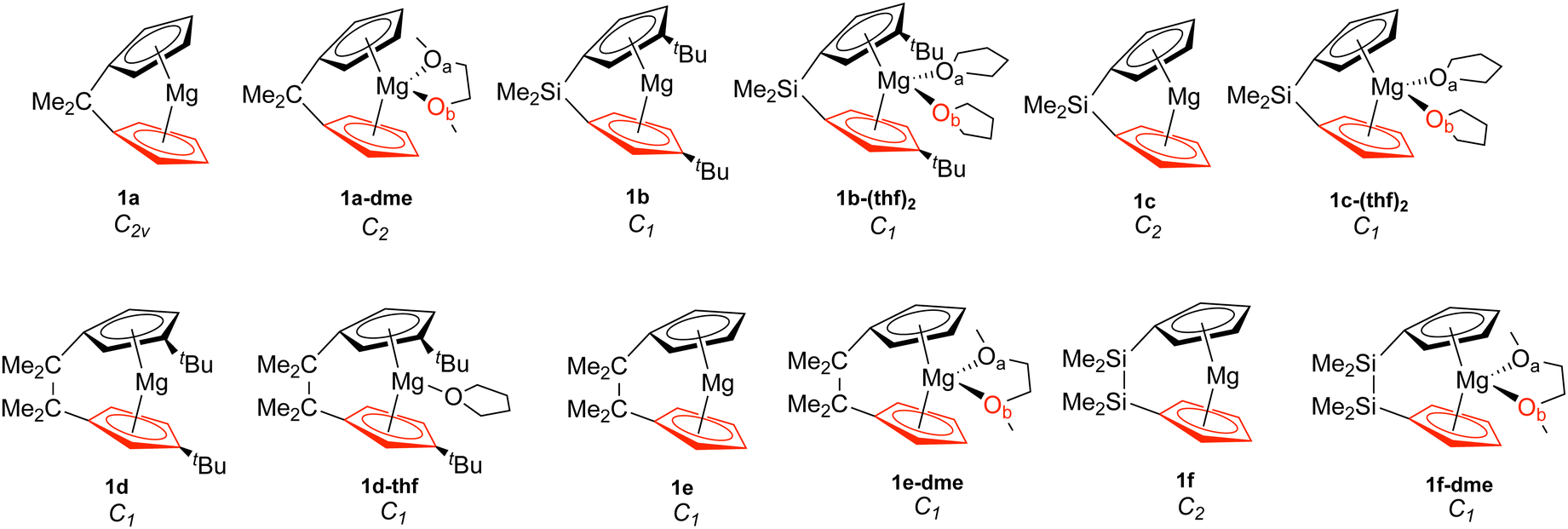 | ||
| Fig. 1 Magnesocenophanes (1). The bottom Cp ring is highlighted in red, while Oa is in black and Ob is in red. | ||
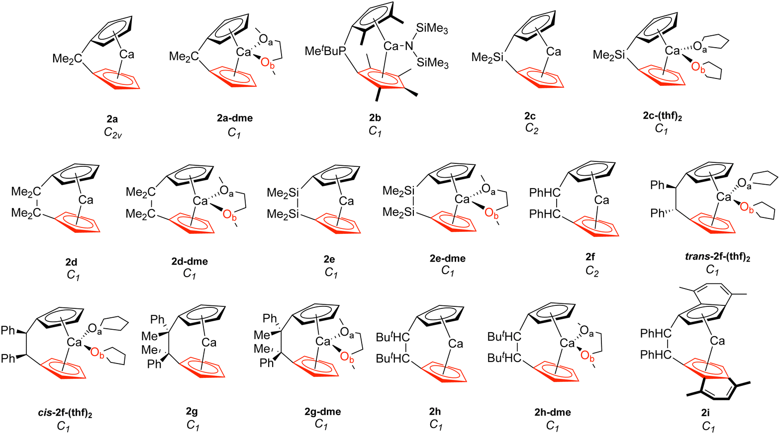 | ||
| Fig. 2 Calcocenophanes (2). The bottom Cp ring is highlighted in red, while Oa is in black and Ob is in red. | ||
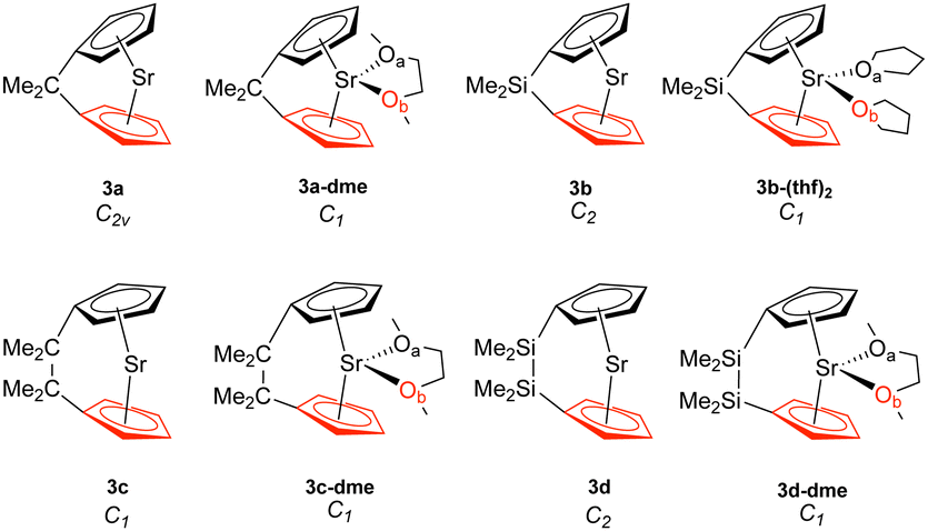 | ||
| Fig. 3 Strontiocenophanes (3). The bottom Cp ring is highlighted in red, while Oa is in black and Ob is in red. | ||
Computational methods
Local mode analysis theory
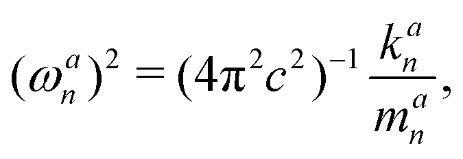
LMA, originally introduced by Konkoli and Cremer,31,32 has evolved over the years into a versatile computational instrument, facilitating the extraction of critical chemical insights from vibrational spectroscopy data. LMA refines the use of normal vibrational force constants and frequencies derived from normal vibrational modes to characterize chemical bonds and/or weak chemical interactions. The normal vibrational modes of a polyatomic molecule are generally delocalized, as stated by Wilson in 1941 via his proof that the associated normal mode coordinates Q are a linear combination of internal coordinates q or Cartesian coordinates x.33 Therefore, normal mode stretching frequencies and associated stretching force constants are of limited use as individual bond strength descriptors. Konkoli and Cremer solved this problem by the transformation of normal vibrational modes into their local mode counterparts.31,32 Mathematical details can be found in two comprehensive review articles.28,29 A local vibrational mode an is defined as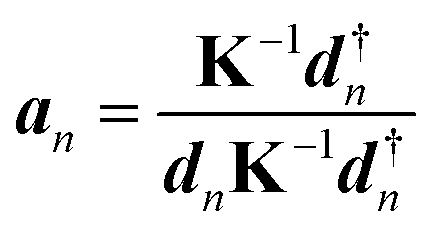 | (1) |
Important to note is that the two ingredients needed for LMA, the diagonal normal mode force constant matrix K in normal mode coordinates Q and the normal mode vectors dn in internal coordinates, can be obtained from a vibrational frequency calculation via the Wilson GF formalism,33–35 a routine part of the most modern quantum chemistry packages.36
The calculation of the corresponding local mode force constant kan can be performed using the following expression:
 | (2) |
This enables the computation of the local mode frequency ωan:
 | (3) |
We have recently developed a unique local mode force constant between the metal and the geometric center of the ring to quantitatively describe metal–π interactions,37 typically found in sandwich compounds38,39 but also in transition metal catalysts40 and enzymes as well.41
In this work, we utilized the local force constant between the metal and the geometric center of the Cp ring, ka(M–Cp), and the local force constant of the angle between the two Cp rings and the metal ka(Cp–M–Cp) as illustrated in Fig. 4.
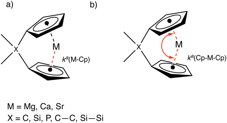 | ||
| Fig. 4 Special force constants used in this work. (a) Local force constant between the metal (M) and geometric centerpoint of the Cp ring ka(M–Cp). (b) Local force constant between the Cp–M–Cp angle ka(Cp–M–Cp). | ||
For the magnesocenophane, calcocenophane and strontiocenophane structures with THF or DME solvent molecules attached to the metal, we have also used the local force constants ka(Mg–O), ka(Ca–O), and ka(Sr–O). These local force constants were transformed into relative bond strength orders (BSOs) according to the generalized Badger rule derived by Cremer, Kraka, and coworkers42,43via a power relationship in the form of BSO = A(ka)B. Two reference molecules with known BSOs and force constants are utilized to obtain the parameters for A and B, with the constraint that a zero value for the force constant ka equals a zero BSO value. To characterize Mg–O interactions, the reference molecules used were MgH2 for the single bond character (BSO = 1) and Mg![[double bond, length as m-dash]](https://www.rsc.org/images/entities/char_e001.gif) O for the double bond (BSO = 2) character,44 with A and B values being 0.7338 and 0.7546, respectively. To characterize Ca–O interactions, the reference molecules used were CaH2 for the single bond character and CaO for the double bond character,45 with A and B values being 1.0391 and 0.4784, respectively. To characterize Sr–O interactions, the reference molecules used were SrH2 for the single bond character and SrO for the double bond character, with A and B values being 1.1409 and 0.4418, respectively. Generally, a discussion in terms of BSO values is chemically more intuitive than the comparison of force constant values.
O for the double bond (BSO = 2) character,44 with A and B values being 0.7338 and 0.7546, respectively. To characterize Ca–O interactions, the reference molecules used were CaH2 for the single bond character and CaO for the double bond character,45 with A and B values being 1.0391 and 0.4784, respectively. To characterize Sr–O interactions, the reference molecules used were SrH2 for the single bond character and SrO for the double bond character, with A and B values being 1.1409 and 0.4418, respectively. Generally, a discussion in terms of BSO values is chemically more intuitive than the comparison of force constant values.
LMA was complemented with the topological analysis of the electron density using Bader's quantum theory of atoms in molecule (QTAIM).46–48 The covalent character of the M–O (where M = Mg, Ca, and Sr) interactions was assessed via the Cremer–Kraka criterion,49,50 which is based on the value of the energy density H(r) taken at the bond critical point rb on the electron density bond path between the two atoms involved in the chemical bond or weak chemical interaction.46–48 A negative value of H(r) indicates the covalent character of the bond/interaction, whereas a positive H(r) value signifies a predominantly electrostatic interaction between the two atoms under consideration. To gain further insight into the electronic structure, specifically with the M–Cp interaction and the effects of the bridging motifs, Laplacian maps were created within the Cp–M–Cp plane. The Laplacian of the electronic density ∇2(ρ(r)) reveals local regions of charge depletion (positive ∇2(ρ(r)) values) and charge concentration (negative ∇2(ρ(r)) values).51,52
Starting geometries of the solvent-bound (THF or DME) ansa-metallocenes were obtained from previous experimental crystal structures.7,15–23 For the structures where no solvent was attached to the group 2 metal, the crystal structure was edited to remove the solvent(s) attached. The geometries and frequencies were calculated for 37 structures ranging from [1]magnesocenophanes, [2]magnesocenophanes, [1]calcocenophanes, [2]calcocenophanes, [1] strontiocenophane, and [2]strontiocenophane, as well as four metallocene structures (ESI,† Fig. S1)30 for comparison (A–D) using the B3LYP functional53,54 with Grimme's D3 dispersion correction zero damping55 (shortened to B3LYP-D3) in combination with the def2-TZVP basis set56 in the gas phase. All DFT calculations were carried out with the Gaussian 16 program57 using an ultrafine grid and a tight convergence criterion for the self-consistent field step. Frequency calculations of all complexes were completed without imaginary normal mode frequencies and followed by subsequent local mode analysis of M–Cp, and M–O bonds, and Cp–M–Cp angles utilizing the LModeA program.58 Natural population charges were calculated utilizing the natural bond orbital (NBO) analysis implemented in the NBO7 program.59 QTAIM calculations were done with the AIMALL package.60
Results and discussion
Table 1 displays the distance d (Å) between the metal and the Cp ring(s) with the corresponding local force constant ka(M–Cp) (mdyn/Å), the angle A (°) for Cp–M–Cp with the corresponding local force constant ka(Cp–M–Cp) (mdynÅ/Rad2), and the natural charge (e) of the metal. For the structures that have distances and local force constants of M–Cp that differ, the top row corresponds to the top Cp ring while the bottom row corresponds to the bottom Cp ring. Fig. 5(a) shows the relationship between the M–Cp bond length and the local force constant and Fig. 5(b) shows the relationship between the Cp–M–Cp bond angle and ka(M–Cp). In Fig. 6(a)–(c), the correlation between the bond length and the local mode force constant is depicted for the Mg–Cp, Ca–Cp, and Sr–Cp bonds, respectively. Table 2 shows BSO n values of M–Oa and M–Ob, distances of M–Oa and M–Ob (Å), local mode force constants ka(M–Oa) and ka(M–Ob), and the angle A (°) between Oa–M–Ob and the corresponding local force constant ka(Oa–M–Ob). Fig. 7(a) and (b) shows BSO n values as a function of the local mode force constants for the Mg–O and Ca–O bonds formed between the metal and THF or DME oxygen(s), respectively. Fig. 7(c) displays the relationship between the energy density H(r) (Hartree/Å3) and the local force constant ka(M–O). Fig. 8(a) shows the relationship between the Cp–M–Cp bond angles and the corresponding local force constant ka(Cp–M–Cp), while Fig. 8(b) displays the relationship between the charge on M and the local force constant ka(Cp–M–Cp). Fig. 9 displays the Laplacian of electronic density ∇2(ρ(r)) for some of the complexes investigated.| Structure | d | k a (M–Cp) | A | k a (Cp–M–Cp) | e |
|---|---|---|---|---|---|
| 1a | 2.003 | 1.551 | 126.6 | 1.043 | 1.776 |
| 1a-dme | 2.156 | 0.321 | 125.3 | 1.021 | 1.811 |
| 1b | 2.000 | 1.578 | 139.4 | 0.805 | 1.816 |
| 1b-(thf)2 | 2.122 | 0.933 | 127.2 | 0.577 | 1.827 |
| 2.188 | 0.370 | ||||
| 1c | 2.004 | 1.539 | 138.9 | 0.806 | 1.794 |
| 1c-(thf)2 | 2.120 | 0.927 | 128.3 | 0.644 | 1.820 |
| 2.165 | 0.308 | ||||
| 1d | 1.975 | 1.735 | 140.2 | 0.737 | 1.825 |
| 1.976 | 1.749 | ||||
| 1d-thf | 2.092 | 1.052 | 135.5 | 0.662 | 1.841 |
| 2.108 | 1.036 | ||||
| 1e | 1.981 | 1.693 | 139.6 | 0.737 | 1.800 |
| 1e-dme | 2.156 | 0.629 | 133.4 | 0.568 | 1.816 |
| 1f | 1.992 | 1.673 | 160.2 | 0.510 | 1.817 |
| 1f-dme | 2.108 | 1.046 | 148.2 | 0.529 | 1.808 |
| 2.241 | 0.370 | ||||
| 2a | 2.310 | 1.450 | 114.6 | 2.092 | 1.726 |
| 2a-dme | 2.361 | 1.157 | 112.8 | 1.992 | 1.719 |
| 2.365 | 1.144 | ||||
| 2b | 2.500 | 0.715 | 117.2 | 1.318 | 1.776 |
| 2.508 | 0.718 | ||||
| 2c | 2.326 | 1.394 | 125.8 | 1.596 | 1.743 |
| 2c-(thf)2 | 2.411 | 1.018 | 122.7 | 1.568 | 1.745 |
| 2.400 | 1.053 | ||||
| 2d | 2.307 | 1.576 | 125.4 | 1.389 | 1.751 |
| 2d-dme | 2.360 | 1.302 | 122.0 | 1.319 | 1.734 |
| 2e | 2.335 | 1.440 | 143.6 | 0.635 | 1.771 |
| 2e-dme | 2.401 | 1.132 | 138.0 | 0.820 | 1.746 |
| 2.400 | 1.128 | ||||
| 2f | 2.316 | 1.536 | 124.8 | 1.415 | 1.748 |
| trans-2f-thf | 2.392 | 1.196 | 120.9 | 1.428 | 1.749 |
| 2.401 | 1.136 | ||||
| cis-2f-thf | 2.387 | 1.191 | 122.0 | 1.344 | 1.750 |
| 2.383 | 1.238 | ||||
| 2g | 2.306 | 1.578 | 125.5 | 1.305 | 1.753 |
| 2.310 | 1.570 | ||||
| 2g-dme | 2.356 | 1.314 | 122.6 | 1.223 | 1.736 |
| 2.367 | 1.296 | ||||
| 2h | 2.296 | 1.585 | 124.5 | 1.36 | 1.751 |
| 2.310 | 1.539 | ||||
| 2h-dme | 2.363 | 1.255 | 121.9 | 1.319 | 1.735 |
| 2.346 | 1.326 | ||||
| 2i | 2.319 | 1.431 | 123.3 | 1.075 | 1.754 |
| 2.312 | 1.425 | ||||
| 3a | 2.485 | 1.310 | 108.1 | 2.441 | 1.757 |
| 3a-dme | 2.535 | 1.094 | 106.4 | 2.292 | 1.760 |
| 2.536 | 1.046 | ||||
| 3b | 2.507 | 1.237 | 118.8 | 1.877 | 1.772 |
| 3b-(thf)2 | 2.579 | 0.964 | 116.3 | 1.724 | 1.778 |
| 2.571 | 0.928 | ||||
| 3c | 2.489 | 1.412 | 118.5 | 1.560 | 1.781 |
| 3c-dme | 2.534 | 1.199 | 116.9 | 1.465 | 1.772 |
| 2.530 | 1.222 | ||||
| 3d | 2.523 | 1.271 | 135.8 | 0.774 | 1.801 |
| 3d-dme | 2.573 | 1.054 | 133.5 | 0.775 | 1.783 |
| 2.570 | 1.085 |
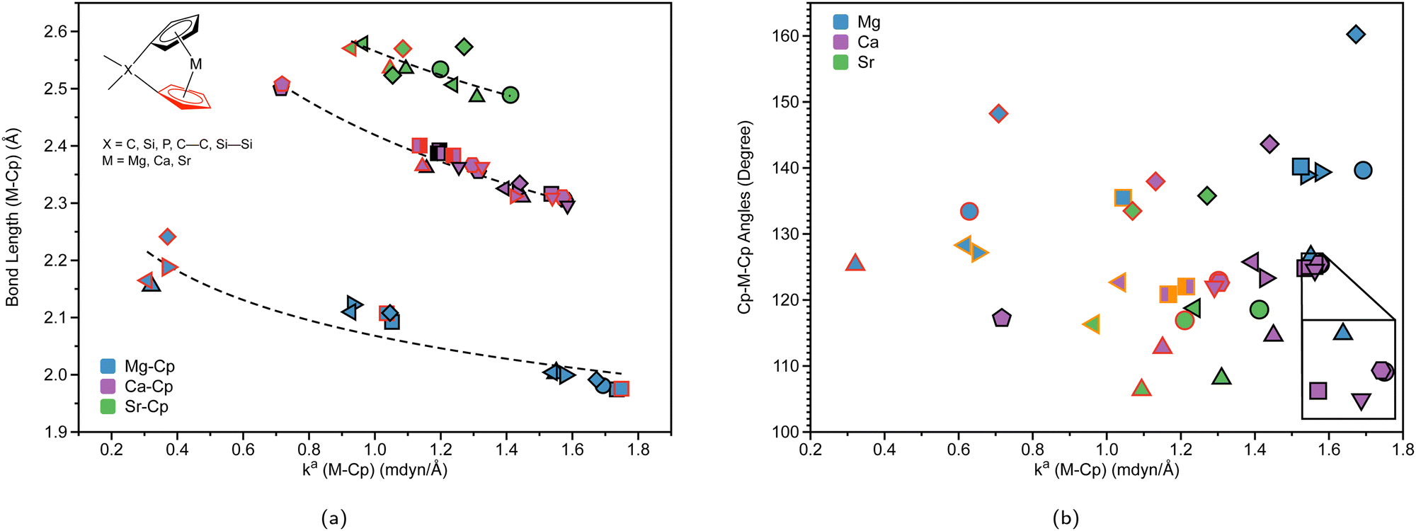 | ||
| Fig. 5 (a) M–Cp bond length (Å) (where M = Mg (blue), Ca (purple), or Sr (green)) vs. local force constant ka(M–Cp) (mdyn/Å). The black outline represents the top portion of the ring and the red outline represents the bottom portion of the Cp ring. The dashed lines for each group are displayed for clarity. (b) Cp–M–Cp angles (degree) vs. local force constant ka(M–Cp) (mdyn/Å). For clarity, the average of the ka(M–Cp) top and bottom rings is displayed. The black outline represents non-solvated structures, the red outline represents DME-solvated structures, and the orange outline represents THF-solvated structures. For more information regarding the symbol labels, the reader is referred to Fig. 6(a) and (b), where the same symbols are utilized at the B3LYP-D3/def2-TZVP level of theory. | ||
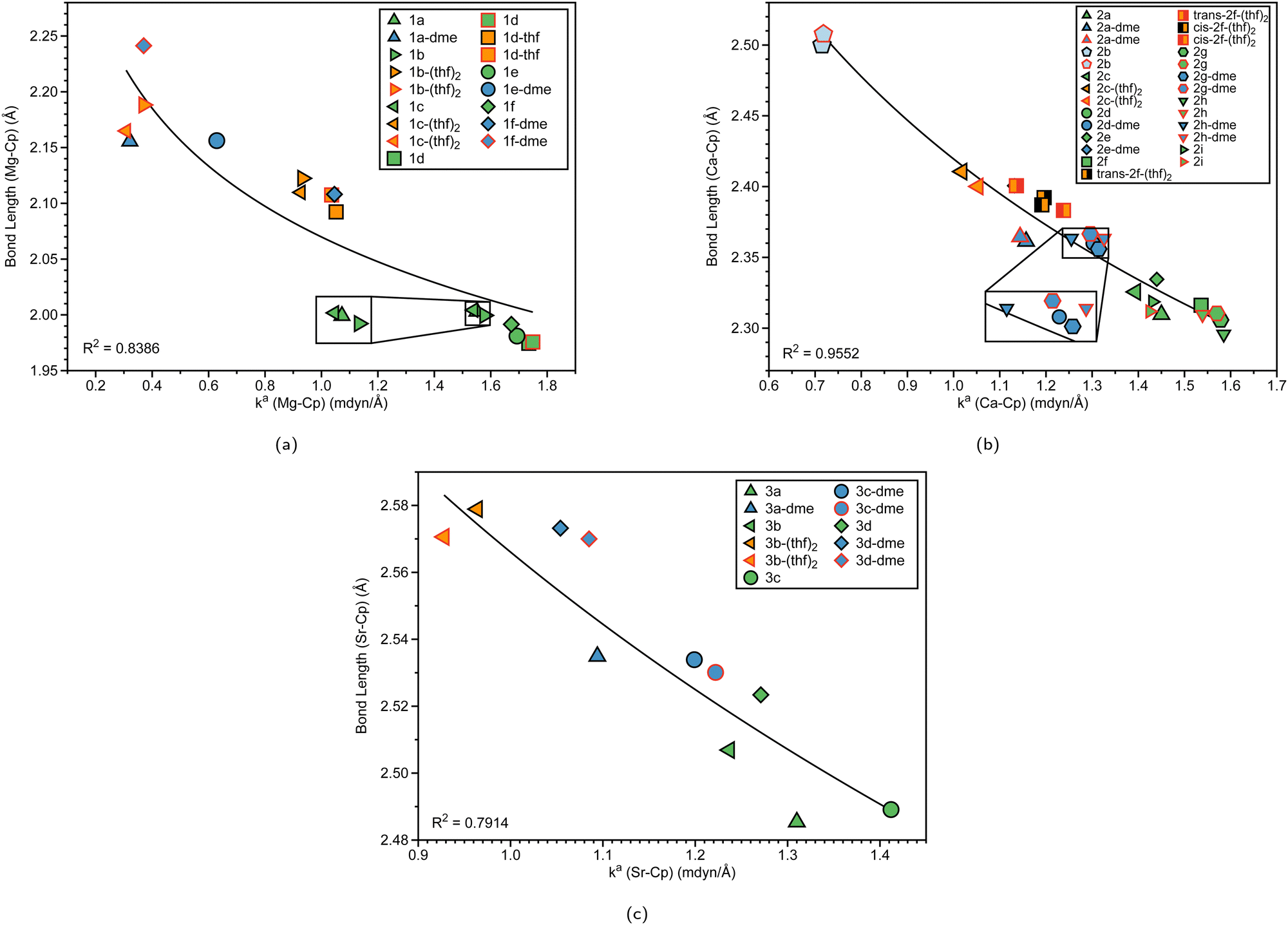 | ||
| Fig. 6 (a) Mg–Cp bond length (Å) vs. local force constant ka (Mg–Cp) (mdyn/Å). (b) Ca–Cp bond length (Å) vs. local force constant ka (Ca–Cp) (mdyn/Å). (c) Sr–Cp bond length (Å) vs. local force constant ka(Sr–Cp) (mdyn/Å). The black outline represents the top portion of the ring and the red outline represents the bottom portion of the Cp ring at the B3LYP-D3/def2-TZVP level of theory. | ||
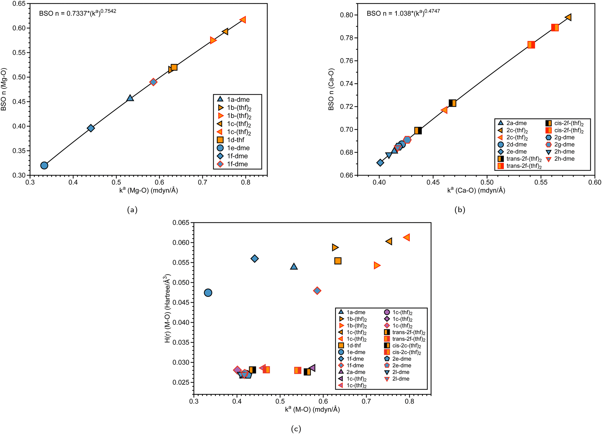 | ||
| Fig. 7 (a) BSO n (Mg–O) vs. local force constant ka(Mg–O) (mdyn/Å). (b) BSO n (Ca–O) vs. local force constant ka(Ca–O) (mdyn/Å). The black outline represents Oa, while the red outline represents Ob (see Fig. 1 and Fig. 2). (c) Energy density H(r) (Hartree/Å3) vs. local force constant ka(M–O) (where M = Mg, Ca). The black outline represents Oa, while the red outline represents Ob at the B3LYP-D3/def2-TZVP level of theory. | ||
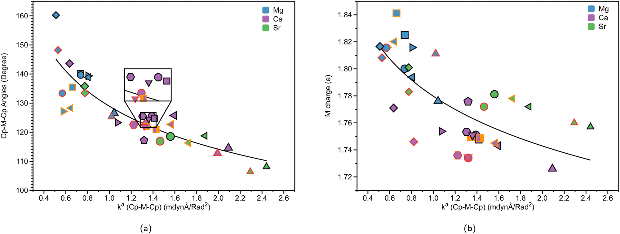 | ||
| Fig. 8 (a) Cp–M–Cp angles (degree), (where M = Mg (blue), Ca (purple), or Sr (green)) vs. local force constant ka(Cp–M–Cp) (mdynÅ/Rad2). (b) NBO charge on M (e) vs. ka(Cp–M–Cp) (mdynÅ/Rad2). The black outline represents non-solvated structures; the red outline represents DME-solvated structures, and the orange outline represents THF-solvated structures at the B3LYP-D3/def2-TZVP level of theory. | ||
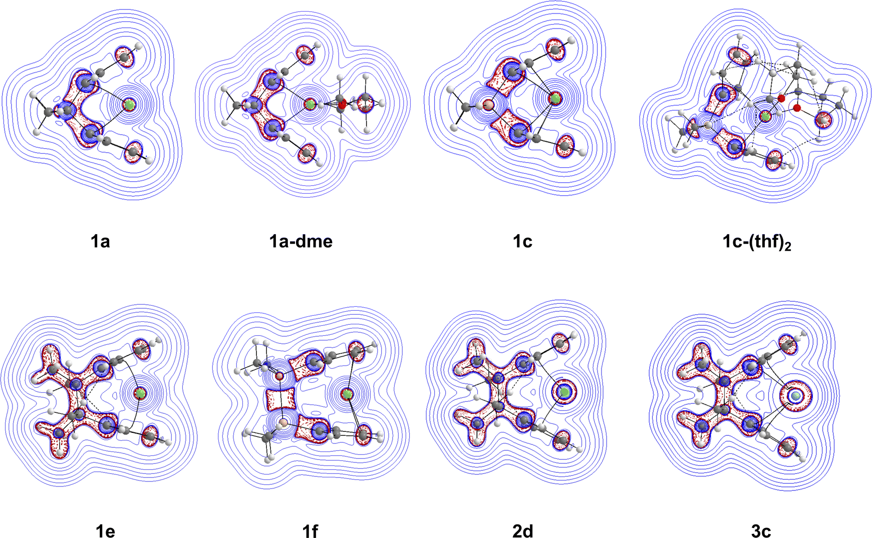 | ||
| Fig. 9 Contour plots displaying the Laplacian of the electron density within the Cp–M–Cp plane for 1a, 1a-dme, 1c, 1c-(thf)2, 1e, 1f, 2d, and 3c. The blue solid lines account for positive ∇2(ρ(r)) values (depletion of the charge)), while the red dashed lines represent negative ∇2(ρ(r)) values (concentration of the charge) at the B3LYP-D3/def2-TZVP level of theory. | ||
M–Cp bond length, Cp–M–Cp bond angle and local mode M–Cp force constant
To investigate the relationship between the nature of group 2 metals and the M–Cp bond in ansa-metallocene structures, the trend between the bond length and the local force constant of M–Cp for group 2 metals (Mg, Ca, and Sr) is plotted in Fig. 5(a). There is an obvious trend between the metal that characterizes the ansa-metallocenes and the distance/local force strength encountered. This trend starts with magnesocenophanes having the metal and Cp rings closer together (with a range from 1.981 to 2.241 Å), and is confirmed by the local force constants, with longer bonds having a lower local force constant and shorter bonds having a higher local force constant. As we go down the periodic table and increase the size of the atom from Mg to Ca, the length of M–Cp increases (with a range from 2.296 to 2.508 Å), which is again confirmed by the local force constants (i.e. longer bonds having a lower force constant). Increasing the size from Ca to Sr, the length of M–Cp increases (with a range from 2.485 to 2.579 Å). It is interesting to note that as the bond length of the M–Cp bond increases as we go down the periodic table, the local force constant does not dramatically change as one might expect. For example, 1e has a bond length of 1.981 Å and a local force constant of 1.673 mdyn/Å, whereas 2d, which has the same [2]carbon bridging motif as 1e, has a bond length of 2.307 Å and a local force constant of 1.576 mdyn/Å. Although there is a slight lengthening of the M–Cp bond from Mg to Ca, the local force constant only slightly decreases in strength. If we go down the periodic table again to Sr (3c), the bond length of the Sr–Cp bond is 2.489 Å, while the local force constant is 1.412 Å, further decreasing slightly in the bond strength as the bond length increases. This is indicative that the strength of the M–Cp bond(s) is not only dependent on the nature of the metal but also dependent on the stability that the bridging motifs bring.For further insight, the relationship between the Cp–M–Cp bond angle and ka(M–Cp) was analyzed, as shown in Fig. 5(b). It appears that there is no general or periodic trend observed concerning the Cp–M–Cp angle and the M–Cp force constant. There is a general effect on the nature of the metal; as one goes from Mg to Sr, the Cp–M–Cp angle decreases, as shown for [2]sila-bridging motifs (139.6° for 1e, 125.4° for 2d, and 118.5° for 3c) and we also see that the M–Cp bond strength effectively decreases (1.981 mdyn/Å, 1.576 mdyn/Å, and 1.412 mdyn/Å, respectively). When looking at qualitative assessments such as an orbital overlap, one can propose that the change of the angle where the metal effectively slips out of the ring changes the overlap between the Cp rings and the metal. With our local force constants as a complementary tool, the changes of the M–Cp strength coupled with the Cp–M–Cp angles can be tracked quantitatively. It is observed that there is a solvation effect, with the binding of THF or DME decreasing the angle and subsequently the bond strength of M–Cp. For magnesocenophanes, the bridging motifs going from [1]sila to [2]carba does not drastically change the angle. For example, 1b and 1c (which are [1]sila magnesocenophanes) have similar angles and ka(M–Cp) bond strengths (139.4°, 1.578 mdyn Å−1 and 138.9°, 1.539 mdyn Å−1, respectively), while 1d and 1e (which are [2]carba-magnesocenophanes) have similar angles and ka (Mg-Cp) average to their [1]sila-counterpart (140.2°, 1.524 mdyn/Å and 139.6°, 1.693 mdyn/Å, respectively). Going from a [2]carba-bridging motif to a [2]sila-motif increases the angle by about 20° for magnesocenophanes. For calcocenophanes, the bridging motifs going from [1]carba to [1]sila (2a to 2c) only changes the angle 10°, with a minimal change in the ka(Ca–Cp) force constant (1.450 mdyn/Å for 2a and 1.394 mdyn/Å for 2c). Going from a [2]carba-motif to a [2]sila-motif (2d to 2e), we see a similar increase in the angle as shown for the one-atom-bridged motif counterpart. The bond strength between the Ca–Cp going from [2]carba to [2]sila slightly decreases (1.576 mdyn/Å for 2d and 1.440 mdyn/Å for 2e). For calcocenophanes, since these structures are primarily experimentally characterized with [2]carba-bridging motifs, the bond angles, as well as the ka(M–Cp) do not differ much for the non-solvated structures (with the only exception being 2i, most likely due to the addition of the ring, and 2e, most likely due to the Si atom).
To gain insight into the effects that solvated structures have in characterizing magnesocenophanes, calcocenophanes, and strontiocenophanes, individual M–Cp bond lengths versus local force constants are displayed in Fig. 6(a) for magnesocenophanes, Fig. 6(b) for calcocenophanes, and Fig. 6(c) for strontiocenophanes. As shown in more detail in Fig. 6(a), the solvent(s) that are typically present in characterizing these magnesium-containing metallocenophane structures through X-ray crystallography (whether THF or DME) drastically affect the strength of the Mg–Cp bond by decreasing the local force constant and increasing the bond length of the Mg–Cp bond(s) compared to its non-solvated counterpart. For example, in 1a, the Mg–Cp distance is 2.003 Å with a force constant of 1.551 mdyn/Å, whereas in 1a-dme, it is 2.156 Å with a force constant of 0.321 mdyn/Å. It is also evident that the effect of binding to THF or DME in magnesocalcenophanes breaks the apparent Mg–Cp symmetry of the structure, as shown in Fig. 6(a), where green colored points indicate non-solvated structures, orange indicates the THF solvent that is bound to the structure(s), and blue indicates the DME solvent that is bound to the structure(s). There is also clustering of the top and bottom Mg–Cp rings for solvent-bound magnesocenophanes (Fig. 6(a), black (top ring) and red (bottom ring) outline for 1b-(thf)2, 1c-(thf)2, 1d-thf, and 1f-dme). It appears that most solvated magnesocenophane structures (except for 1a-dme and 1e-dme) have the top Cp ring closer to the Mg metal (an average of 2.108 Å) and the stronger local force constant (an average of 0.989 mdyn/Å) than the bottom Cp ring (which has average values of 2.175 Å and 0.521 mdyn/Å). It is important to note the significance of the decrease in the local force constant and an increase in the bond length for the solvent-coordinated Mg–Cp rings since these compounds are usually characterized as intermediates in catalysis to prepare transition metal metallocenophanes.24 Utilizing the LMA, it is observed that the solvent-coordinated magnesium-containing ansa-metallocenophanes have a weaker local force constant than its non-solvated counterpart, allowing for Mg to be replaced with a transition metal with more ease. This makes the LMA a powerful tool to capture the strong influence that solvent coordination can have on the overall geometry and ability of magnesocenophanes to be used in transmetalation reactions.
Similar to the magnesocenophane trend that was seen for solvent-containing compounds, solvent-bound calcocenophanes show a slight decrease in the local force constant ka(Ca–Cp) and bond length as shown in Fig. 6(b). There is a trend between the solvated structures and the non-solvated structures, with the THF solvated structures (2c-(thf)2, trans-2f-(thf)2 and cis-2f-(thf)2) grouped (an average M–Cp bond length of 2.396 Å and a force constant of 1.139 mdyn/Å), and the DME solvated structures (2e-dme, 2g-dme and 2h-dme) grouped (an average bond length of 2.372 Å and a force constant of 1.242 mdyn/Å). The only outlier that is not grouped in its appropriate solvation group is 2d-dme, the [2]carba-calcocenophane motif, which has a bond length of 2.360 Å and a strength of 1.302 mdyn/Å, which is higher than the DME Ca–Cp average. It is important to note that structure 2b (the light blue pentagon in Fig. 6(b)) does have an amide group attached to the calcium, has phosphorus as the bridging atom, and instead of the typical Cp ring that is utilized for ansa-metallocenes, is pentamethyl cyclopentadiene (Cp*). Unlike the magnesocenophane non-solvated structures, the calcocenophane structures that are not solvated have slightly different Ca–Cp bond lengths/force constants, displaying a lack of symmetry in these structures. This could be due to its primary bridging motif, which, unlike magnesocenophanes, comprises mostly [2]carba-calcocenophanes, with different branching points from the carbon, such as the addition of phenyl groups (2f, trans-2f-(thf)2, cis-2f-(thf)2, and 2i), methyl and phenyl groups (2g) and tert-butyl groups (2h and 2h-dme). Similar to magnesocenophanes, the synthetic uses of these calcocenophanes are typical for transmetalation reactions and are typically seen as an impurity when carrying out reductive elimination reactions.20
Although we see a similar trend between the non-solvated and the solvated strontiocenophanes, it is not as separated as seen for the magnesocenophane and calcocenophanes, as shown in Fig. 6(c). The strongest and shortest non-solvated Sr–Cp bond is the [2]carba-bridged motif 3c (2.489 Å and 1.412 mdyn/Å), with the weakest and longest non-solvated Sr–Cp bond is the [2]sila-bridged motif 3d (2.523 Å and 1.271 mdyn/Å). Solvation further decreases the bond strength, however, not as much, with the strongest solvated Sr–Cp bond coming from 3c-dme (an average of 1.211 mdyn/Å between the two rings). Overall, the weakest Sr–Cp bond comes from the [1]sila-motif with solvation (3c-(thf)2), an average of 0.946 mdyn/Å between the two rings, with a bond length of 2.575 Å. It appears that the one-atom-bridged silicon, coupled with solvation, decreases the strength for the M–Cp bond, which was also seen for magnesocenophanes (1e-dme) and calcocenophanes (when disregarding 2b, 2c-(thf)2).
Mg–O and Ca–O interactions with solvent molecules
To further investigate the effect of the solvent(s) (THF or DME) binding to group 2 ansa-metallocenes, we have plotted the BSO of the Mg–O and Ca–O interactions with respect to the local force constant (mdyn/Å) in Fig. 7(a) and (b), respectively. Table 2 also displays information on the bond distances, angles, and force constants of the M–Oa and M–Ob bonds, including Sr–O. If a structure is bound to two oxygens that have different corresponding bond strengths, the oxygens are labeled in Fig. 1–3, where Oa is indicated as a black outline, and Ob is indicated as a red outline. For the solvent-bound magnesocenophane systems in Fig. 7(a), most of the systems (except for 1d-thf) have two oxygens bound to Mg. For the other DME solvated structure, 1f-dme, Mg–Oa has a BSO of 0.440 and a local force constant of 0.396 mdyn/Å, whereas for Mg–Ob, the local force constant and BSO increase (0.586 mdyn/Å and 0.490 respectively). The same trends are seen for THF-solvated structures, where the Mg–Oa bond has a smaller BSO and local a force constant, indicating that it is weaker than its Mg–Ob counterpart. It is also interesting to note that the DME-bound structures have weaker Mg–O bonds and the THF-solvated systems have stronger Mg–O bonds. A previous experimental investigation for dehydrocoupling reactions in [1]carba magnesocenophanes showed that the catalytic activity was lower in THF complexes than that in DME complexes, which our theoretical insight supports.15 For solvated calcocenophanes, as shown in Fig. 7(b), similar trends are seen as previously described in solvated magnesocenophane systems, where Ca–Oa bonds are weaker than the Ca–Ob bonds. However, for 2g-dme and 2h-dme, going from Ca–Oa to Ca–Ob slightly increases in the bond strength (0.008 mdyn/Å increase) and for trans-2f-(thf)2 and cis-2f-(thf)2, it increases a bit more (0.105 mdyn/Å and 0.095 mdyn/Å increase, respectively). While there are not many solvated molecules for the strontiocenophanes, looking at Table 2 shows that the same trend still applies, with only the M–Ob bond from 3d-dme having a similar bond strength to that from 3b-(thf)2. We also see for THF structures, the Oa–M–Ob bond is greater than DME structures, which is also indicated by weaker local force constants (which indicates a less stiff bond, whereas for the DME structures, the angles are much more acute, followed by a greater local force constant for the angle). Overall, as reflected by the BSO values, the Mg–O and Ca–O interactions are weaker than a single bond.| Structure | BSO n (M–Oa) | BSO n (M–Ob) | d (M–Oa) | d (M–Ob) | k a (M–Oa) | k a (M–Ob) | A | k a (Oa–M–Ob) |
|---|---|---|---|---|---|---|---|---|
| 1a-dme | 0.456 | 0.456 | 2.126 | 2.126 | 0.532 | 0.532 | 76.3 | 1.486 |
| 1b-(thf)2 | 0.515 | 0.575 | 2.110 | 2.083 | 0.626 | 0.723 | 91.8 | 0.500 |
| 1c-(thf)2 | 0.593 | 0.617 | 2.072 | 2.068 | 0.754 | 0.795 | 88.0 | 0.531 |
| 1d-thf | 0.520 | 2.096 | 0.634 | |||||
| 1e-dme | 0.320 | 0.320 | 2.186 | 2.187 | 0.333 | 0.333 | 73.9 | 1.350 |
| 1f-dme | 0.396 | 0.490 | 2.170 | 2.107 | 0.441 | 0.586 | 75.1 | 1.455 |
| 2a-dme | 0.681 | 0.681 | 2.470 | 2.472 | 0.414 | 0.414 | 68.3 | 1.341 |
| 2c-(thf)2 | 0.798 | 0.717 | 2.401 | 2.442 | 0.576 | 0.461 | 79.3 | 0.369 |
| 2d-dme | 0.687 | 0.687 | 2.479 | 2.479 | 0.421 | 0.421 | 67.9 | 1.418 |
| 2e-dme | 0.671 | 0.671 | 2.481 | 2.484 | 0.401 | 0.401 | 67.7 | 1.449 |
| trans-2f-(thf)2 | 0.699 | 0.774 | 2.453 | 2.420 | 0.436 | 0.541 | 79.4 | 0.326 |
| cis-2f-(thf)2 | 0.789 | 0.723 | 2.405 | 2.434 | 0.563 | 0.468 | 79.6 | 0.347 |
| 2g-dme | 0.691 | 0.685 | 2.476 | 2.478 | 0.426 | 0.418 | 67.9 | 1.431 |
| 2h-dme | 0.678 | 0.684 | 2.481 | 2.479 | 0.409 | 0.417 | 67.9 | 1.408 |
| 3a-dme | 0.734 | 0.658 | 2.646 | 2.711 | 0.369 | 0.288 | 63.2 | 1.422 |
| 3b-(thf)2 | 0.786 | 0.718 | 2.598 | 2.641 | 0.430 | 0.351 | 77.0 | 0.301 |
| 3c-dme | 0.694 | 0.693 | 2.672 | 2.675 | 0.325 | 0.324 | 63.6 | 1.424 |
| 3d-dme | 0.715 | 0.719 | 2.658 | 2.657 | 0.347 | 0.352 | 64.0 | 1.463 |
We also investigated the covalent character of the M–O bond via the inspection of the electron density H(r). Fig. 7(c) shows the relationship between H(r) (M–O) and the local force constant ka(M–O), with the black outline representing Oa and the red outline representing Ob. It is apparent that the magnesocenophane metal–oxygen bonds have more electrostatic characters than the calcocenophane counterparts. For magnesocenophanes, when going from Mg–Ob to Mg–Oa, the electrostatic character typically increases (except for 1c-(thf)2, where it decreases) as the local force constant decreases. Overall, for calcocenophanes, H(r) values are similar to those of DME and THF-bound oxygen, a trend which is also seen in Fig. 7(b).
Cp–M–Cp angle bending and stiffness
To explore the correlation between Cp–M–Cp angles and the relative stiffness of ansa-metallocenes, the LMA was conducted on the systems investigated. Fig. 8(a) presents the relationship between the bond angles of Cp–M–Cp for the group 2 metals (Mg (blue), Ca (purple), and Sr (green)) and its local force constant counterpart. Fig. 8(b) shows the relationship between the charge of the group 2 metal (e) and the local force constant ka(Cp–M–Cp) indicating the stiffness of the angle indicated. The black outline in Fig. 8(a) and (b) refers to non-solvated structures, whereas the red outline represents DME-solvated structures, and the orange outline represents THF-solvated structures. The Cp–Mg–Cp angles in magnesocenophanes range from 125.4° to 160.2°. For magnesium-containing ansa-metallocenes, the non-solvated structures (black outline) show a trend that as the angle between the Cp–Mg–Cp bond decreases, the force constant increases. The effect of the [1]carba/[1]sila magnesocenophanes and [2]carba/[2]sila magnesocenophanes bridging motifs is evident in these trends. For example, going from [1]carba magnesocenophane 1a to [1]sila magnesocenophane 1c increases the bond angle from 126.6° to 138.9°, which is reflected by the decrease in the local force constant (1.043 mdynÅ/Rad2 to 0.806 mdynÅ/rad2). This trend is also seen going from [2]carba magnesocenophane 1e to [2]sila magnesocenophane 1f. What the local force constant from LMA captures is the ability to measure stiffness and compare these bond angles amongst each other, as we see here with the stiffness decrease as we change the bridging motif atom from carbon to silicon. Therefore, one could propose that if one wants a very stiff magnesocenophane structure, utilizing a [1]carba-bridging motif will yield beneficial results, whereas if one wants a more relaxed Cp–Mg–Cp angle, the [2]sila-bridged magnesocenophane would be the most optimal option. The effect that solvation has on the stiffness of the Cp–Mg–Cp angle is evident as well, showing that the local force constant and angle decrease for solvent-coordinated structures. For example, 1d (blue square, black outline) has an angle of 140.2° and a local force constant of 0.737 mdynÅ/Rad2, whereas 1d-thf (blue square, orange outline) has an angle of 135.5° and a local force constant of 0.662 mdynÅ/rad2.For calcocenophanes, the angles range from 114.6° to 143.6°. We see a similar trend that as the angle increases, the force constant decreases for non-solvated structures (black outline). Going from [1]carba calcocenophane 2a to [1]sila calcocenophane 2c increases the bond angle from 114.6° to 125.8°, with a decrease in the local force constant (2.092 mdynÅ/Rad2 to 1.596 mdynÅ/rad2). When one goes from a [2]carba calcocenophane 2d to a [2]sila calcocenophane 2e, the angle also increases as well from 125.4° to 143.6° (with a decrease in the local force constant of the Cp–M–Cp angle). It is important to note that most structures have different substituents on the Cp ring and bridging motifs among the [2]carba-calcocenophanes, particularly 2f–2i. The same trend where the angle increases going from a one-atom to two-atom bridged motif that was seen for [2]carba/sila magnesocenophanes is also seen for [2]carba/sila calcocenophanes. Considering solvation effects, LMA does capture the differences in the bond angle stiffness as one goes from non-solvated structures to solvated structures. The same trend seen in magnesocenophanes with regard to solvated structures is seen with calcocenophanes. For example, going from 2g (purple pentagon, black outline), which has an angle of 122.6° and a local force constant of 1.360 mdyn Å rad−2, to DME-solvated 2g-dme (purple pentagon, red outline) decreases the angle and force constant (121.9° and 1.319 mdynÅ/Rad2, respectively). This angle and local force constant decrease from non-solvated to solvated structures is seen in both magnesocenophanes and calcocenophanes alike. It is also interesting to note that the [2]carba calcocenophanes that have a phenyl ring attached to the carbons instead of a methyl group (2f, trans-2f-(thf)2, cis-2f-(thf)2, 2g, 2g-dme, 2h, 2h-dme, and 2i) all have similar bond angles 120°–124°, most likely due to the rigidity and the steric effects of the motifs.
For strontiocenophanes, the same trend is observed, with the range of Cp–M–Cp angles being from 106.4° to 135.8°. Going from a [1]carba strontiocenophane to a [1]sila strontiocenophane increases the angle from 108.1° to 118.8°, which is reflected with the decrease in the corresponding local force constant (2.441 mdynÅ/Rad2 to 1.877 mdynÅ/Rad2). Overall, the stiffness of the Cp–M–Cp increases as you go down the group 2 metals (from Mg (blue), Ca (purple) to Sr (green)), as exhibited by the local force constant for Cp–M–Cp increasing with the bond angle decreasing as well. Fig. 8(a) displays that there is no periodic trend as observed previously; however, there are similar groupings based on the bridging motif (for example, the [2]sila calcocenophane/[2]sila strontiocenophane indicated by diamond purple and diamond green, respectively). Previous computational investigation into group 2 metallocenes without the ansa-bridging motif displays similar trends as one goes down the group 2 periodic table, the angle between the Cp–M–Cp decreases, losing its linear structure (∼180°) and becoming more bent.61
As shown in Fig. 8(b), which shows the charge of the metal corresponding with the stiffness of the Cp–M–Cp bond (ka(Cp–M–Cp)), there appears to be not much of a periodic trend between the angle of Cp–M–Cp and stiffness (ka(Cp–M–Cp)), indicating that the bridging motifs, as well as the solvation of THF or DME can affect the stiffness of the Cp–M–Cp angle, and the charge of the atom. Another interesting thing to note is that for magnesocenophanes, the addition of solvation appears to slightly increase the charge of the metal (the red/orange outline is a greater charge in Fig. 8(b) than the black outline). For calcocenophanes, it appears that this is not the trend observed, with the majority of solvated molecules having a slight decrease in charge. For strontiocenophanes, there is not much change that occurs due to solvation. Going from one-atom to two-atom bridging, regardless of whether it is carbon or silicon, slightly increases the charge of the metal. Overall, utilizing LMA can quantitatively display the differences in bridging motifs, solvation, and even substituents on the Cp ring, which change the stiffness of the Cp–M–Cp angle, as well as the charge of the metal.
To further elucidate the Cp–M–Cp interaction and the effects of the bridging motifs, ∇2(ρ(r)) maps were created within the Cp–M–Cp plane. The Laplacian contour plots of complexes 1a, 1a-dme, 1c, 1c-(thf)2, 1e, 1f, 2d, and 3c are shown in Fig. 9(b). The Laplacian contour plots of selected complexes can be found in the ESI† (Fig. S2 and S3). Going from the non-solvated 1a structure to the solvated 1a-dme structure does not change the distribution of the Laplacian very much around the bridging motif and the ring structures. However, the effect of going from [1]carba-1a to [1]sila-1c bridging motifs is evident with the difference in the distribution of the Laplacian. In 1a, there is local electron density distribution (charge concentration, indicated by the red dashed lines) between the bonds of the bridging motifs, whereas in 1c, there is significantly greater charge depletion (indicated by the blue solid lines) around the silicon atom compared to the carbon atom. Going from the non-solvated 1c to the solvated 1c-(thf)2 structures, there is also a change in the Laplacian distribution, most likely due to the non-covalent interactions that are occurring between the solvent (THF) and the Cp rings. The difference in the contour map is also apparent going from [1]carba- to [2]carba-bridging motifs, with there being more charge concentrations occurring between the bonds in the bridging motif (1e). As seen before when changing from carbon to silicon, having a [2]sila-bridging motif (1f) allows for greater charge depletion around the silicon atoms, with the charge concentration occurring between the two silicon atoms. Finally, for 2d and 3c, the Laplacian of the electronic density is very similar to that of the [2]carba magnesocenophane (1e), with the only difference coming from the metal, with 2d having more charge concentrations around its metal center, and 3c having even more charge concentrations. Overall, the electronic density shows that the metal–oxygen bond is of electrostatic character, while the contour maps display the differences between bridging motifs and metal centers, giving a more detailed insight into the electronic structure of the ansa-metallocene structures investigated.
Bent versus linear metallocenes
To further see the effects that the bridging motifs have on the ansa-metallocene structures, four metallocene compounds (labeled as A–D, see the ESI,† Fig. S1) were investigated (with the structures taken from a previous computational investigation from Pal et al.)30 for comparison of the magnesocenophane and calcocenophane structures. There are three linear structures, MgCp2 (A), MgCp*2 (B), and CaCp2 (C), with one bent structure, CaCp*2 (D). Comparing the local force constants ka (M–Cp) of the magnesocenophanes with the corresponding metallocene complex A (1.680 mdyn/Å), it appears that the [1]carba/[1]sila magnesocenophanes have a weaker Mg–Cp bond (with a corresponding slightly longer Mg–Cp bond length), whereas the [2]carba/[2]-sila have a stronger Mg–Cp bond (except for the THF-solvated 1d-thf complex). However, for B (1.789 mdyn/Å), all the magnesocenophanes have a weaker Mg–Cp bond than the metallocene MgCp*2 (B), most likely this is due to the methylated substituents on the Cp ring. For structure C which has a force constant of 1.439 mdyn/Å, the structures that have a stronger Ca–Cp bond are 2d, 2f, 2g, and 2h. For structure D, the only structure that has the Cp* ring motif is 2b, which has a weaker Ca–Cp bond, most likely due to the amide group attached to the calcium atom. Again, the effect of a solvent decreases the bond strength, where the weaker M–Cp bonds compared to the metallocene counterparts come from (i) single-bridged carbon, silicon, and phosphorus (from 2b) motifs and (ii) THF or DME solvated structures, drastically affecting the strength of the M–Cp bond. Interestingly, the CaCp*2 (D) bond angle (155.1°) is much greater than all of the calcocenophanes, showing that the angle of the metallocene can be drastically affected if an ansa-motif is attached to it.Conclusions
In this investigation, we have applied LMA as a quantitative bond strength for metal–π rings to 37 ansa-metallocene structures with group 2 metals ranging from non-solvated to solvated structures with donor solvents (THF and DME) and with different interannular motifs (carba- or sila-motifs with either single or double bridges). We first studied the overall effect of the M–Cp bond strength as one goes down the periodic table from Mg through Sr and confirmed that the M–Cp bond lengths from Mg to Sr increase; however, the local force constant does not drastically decrease, displaying that the strength of the M–Cp bond(s) is not dependent solely on the nature of the metal, but also dependent on the stability that is provided by the bridging motifs. We then studied the differences between non-solvated structures and solvated structures (which are usually characterized experimentally) utilizing the M–Cp bond strength, Cp–M–Cp angles, NBO charge of the metal, and Cp–M–Cp angle stiffness. Our findings indicate that the donor solvent makes a drastic change in the strength of the M–Cp bond and the stiffness of the Cp–M–Cp angle, mainly, that the coordination of the solvent inserted into the ansa-metallocenes drastically decreases the strength of the M–Cp bond and the stiffness of the Cp–M–Cp angle compared to its non-solvated counterpart. Furthermore, when investigating the metal–oxygen bond strengths between THF and DME solvents, it was discovered that DME has weaker metal–oxygen bonds than THF. Also, LMA was able to capture the ability to measure stiffness amongst different bridging motifs. These trends indicate that the silicon bridging atom(s), specifically the [2]sila-bridging motif, greatly increases the Cp–M–Cp angle. This would indicate that the silicon atom would be the best for transmetalation reactions since it decreases the bond strength and increases the bond angle for it to be more easily replaceable with its transition metal counterpart. To further investigate the electronic structure of the ansa-metallocene structures, QTAIM analysis was performed to calculate the energy density of the metal–oxygen bond and the Laplacian of the electronic density, which further supported the effects of solvated ansa-metallocenes and the nature of the bridging motifs. Comparing the linear/bent metallocene complexes, we see the general effect that the ansa interannular motif has on the strength of the M–Cp bond, as well as the effect of solvation, generally decreasing the bond strength. Overall, utilizing a robust computational tool set and including LMA can allow those who are interested in characterizing structures such as ansa-metallocenes a more efficient and quantitative way to calculate metal–π bond strengths, solvent effects, and effects of bridging motifs.Conflicts of interest
There are no conflicts to declare.Acknowledgements
This work was supported by the National Science Foundation, Grant CHE 2102461, and the National Science Foundation Graduate Research Fellowship Program under Grant No. DGE-2034834. We thank the Center for Research Computation at SMU for providing generous high–performance computational resources. J. J. A. thanks Barbara M. T. C. Peluzo for their valuable insight into the Laplacian plots.Notes and references
- L. Resconi, L. Cavallo, A. Fait and F. Piemontesi, Chem. Rev., 2000, 100, 1253–1345 CrossRef CAS PubMed.
- M. Bochmann, J. Organomet. Chem., 2004, 689, 3982–3998 CrossRef CAS.
- M. V. Kharlamova and C. Kramberger, Nanomaterials, 2023, 13, 774 CrossRef CAS PubMed.
- Z. Xin, Y.-R. Wang, Y. Chen, L.-Z. Dong and Y.-Q. Lan, Nano Energy, 2020, 67, 104233 CrossRef CAS.
- Y. Zhao, X. Xu, Y. Wang, T. Liu, H. Li, Y. Zhang, L. Wang, X. Wang, S. Zhao and Y. Luo, RSC Adv., 2022, 12, 21111–21121 RSC.
- V. M. Rayón and G. Frenking, Chem. – Eur. J., 2002, 8, 4963 CrossRef.
- E. D. Brady, S. C. Chmely, K. C. Jayaratne, T. P. Hanusa and V. G. Y. Jr., Organometallics, 2008, 27, 1612–1616 CrossRef CAS.
- S. J. Grabowski and R. D. Parra, Molecules, 2022, 27, 6269 CrossRef CAS PubMed.
- S. Baguli, S. Mondal, C. Mandal, S. Goswami and D. Mukherjee, Chem. – Asian J., 2022, e202100962 CrossRef CAS PubMed.
- P. J. Shapiro, Coord. Chem. Rev., 2002, 231, 67–81 CrossRef CAS.
- C. E. Zachmanoglou, A. Docrat, B. M. Bridgewater, G. Parkin, C. G. Brandow, J. E. Bercaw, C. N. Jardine, M. Lyall, J. C. Green and J. B. Keister, J. Am. Chem. Soc., 2002, 124, 9525–9546 CrossRef CAS PubMed.
- A. Cicolella, E. Romano, V. Barone, C. D. Rosa and G. Talarico, Organometallics, 2022, 41, 3872–3883 CrossRef CAS.
- M. A. Bau, S. Wiesler, S. L. Younas and J. Streuff, Chem. – Eur. J., 2019, 25, 10531–10545 CrossRef CAS PubMed.
- M. Kessler, S. Hansen, C. Godemann, A. Spannenberg and T. Beweries, Chem. – Eur. J., 2013, 19, 6350–6357 CrossRef CAS PubMed.
- L. Wirtz, W. Haider, V. Huch, M. Zimmer and A. Schäfer, Chem. – Eur. J., 2020, 26, 6171–6184 Search PubMed.
- H.-R. H. Damrau, A. Geyer, M.-H. Prosenc, A. Weeber, F. Schaper and H.-H. Brintzinger, J. Organomet. Chem., 1998, 553, 331–343 CrossRef CAS.
- P. Perrotin, B. Twamley and P. J. Shapiro, Acta Crystallogr., Sect. E: Struct. Rep. Online, 2007, 63, m1277–m1278 CrossRef CAS.
- W. Haider, V. Huch and A. Schäfer, Dalton Trans., 2018, 47, 10425–10428 RSC.
- M. Rieckhoff, U. Pieper, D. Stalke and F. T. Edelmann, Angew. Chem. Int. Ed. Engl., 1993, 32, 1079–1081 CrossRef.
- K. M. Kane, P. J. Shapiro, A. Vji, R. Cubbon and A. L. Rheingold, Organometallics, 1997, 16, 4567–4571 CrossRef CAS.
- G. J. Matare, K. M. Kane, P. J. Shapiro and A. Vij, J. Chem. Crystallogr., 1998, 28, 731–734 CrossRef CAS.
- B. Twamley, G. J. Matare, P. J. Shapiro and A. Vij, Acta Crystallogr., Sect. E: Struct. Rep. Online, 2001, 57, m402–m403 CrossRef CAS.
- P.-J. Sinnema, B. Höhn, R. L. Hubbard, P. J. Shapiro, B. Twamley, A. Blumenfeld and A. Vij, Organometallics, 2002, 21, 182–191 CrossRef CAS.
- L. Wirtz and A. Schäfer, Chem. – Eur. J., 2021, 21, 1219–1230 CrossRef PubMed.
- H.-R. H. Damrau, A. Geyer, M.-H. Prosenc, A. Weeber, F. Schaper and H.-H. Brintzinger, J. Organomet. Chem., 1998, 553, 331–343 CrossRef CAS.
- L. Wirtz, J. Lambert, B. Morgenstern and A. Schäfer, Organometallics, 2021, 40, 2108–2117 CrossRef CAS.
- L. Wirtz, K. Y. Ghulam, B. Morgenstern and A. Schäfer, ChemCatChem, 2022, 14, e202201007 CrossRef CAS.
- E. Kraka, M. Quintano, H. W. L. Force, J. J. Antonio and M. Freindorf, J. Phys. Chem. A, 2022, 126, 8781–8900 CrossRef CAS PubMed.
- E. Kraka, W. Zou and Y. Tao, Wiley Interdiscip. Rev.: Comput. Mol. Sci., 2020, 10, 1480 Search PubMed.
- R. Pal, S. Mebs, M. W. Shi, D. Jayatilaka, J. M. Krzeszczakowska, L. A. Malaspina, M. Wiecko, P. Luger, M. Hesse, Y.-S. Chen, J. Beckmann and S. Grabowsky, Inorg. Chem., 2018, 57, 4906–4920 CrossRef CAS PubMed.
- Z. Konkoli and D. Cremer, Int. J. Quantum Chem., 1998, 67, 1–9 CrossRef CAS.
- Z. Konkoli, J. A. Larsson and D. Cremer, Int. J. Quantum Chem., 1998, 67, 11–27 CrossRef CAS.
- E. B. Wilson, J. Chem. Phys., 1941, 9, 76–84 CrossRef CAS.
- J. D. Kelley and J. J. Leventhal, Problems in Classical and Quantum Mechanics: Normal Modes and Coordinates, Springer, 2017, pp. 95–117 Search PubMed.
- E. B. Wilson, J. C. Decius and P. C. Cross, Molecular Vibrations: The Theory of Infrared and Raman Vibrational Spectra, McGraw-Hill, New York, 1955 Search PubMed.
- V. Barone, S. Alessandrini, M. Biczysko, J. R. Cheeseman, D. C. Clary, A. B. McCoy, R. J. DiRisio, F. Neese, M. Melosso and C. Puzzarini, Nat. Rev. Methods Primers, 2021, 1, 38 CrossRef CAS.
- W. Zou, M. Freindorf, V. Oliveira, Y. Tao and E. Kraka, Can. J. Chem., 2023, 101, 616–632 CrossRef.
- M. Z. Makos, W. Zou, M. Freindorf and E. Kraka, Mol. Phys., 2020, e1768314 CrossRef.
- B. M. T. C. Peluzo, M. Z. Makos, R. T. Moura Jr., M. Freindorf and E. Kraka, Inorg. Chem., 2023, 62, 12510–12524 CrossRef CAS PubMed.
- E. Kraka, J. J. Antonio and M. Freindorf, Chem. Commun., 2023, 59, 7151–7290 RSC.
- J. J. Antonio and E. Kraka, Biochemistry, 2023, 62, 2325–2337 CrossRef CAS PubMed.
- D. Cremer and E. Kraka, Curr. Org. Chem., 2010, 14, 1524–1560 CrossRef CAS.
- E. Kraka, J. A. Larsson and D. Cremer, Computational Spectroscopy, Wiley, New York, 2010, pp. 105–149 Search PubMed.
- A. A. A. Delgado, D. Sethio and E. Kraka, Inorganics, 2021, 9, 1–18 CrossRef.
- A. A. A. Delgado, D. Sethio, I. Munar, V. Aviyente and E. Kraka, J. Chem. Phys., 2020, 153, 1–11 CrossRef PubMed.
- R. F. W. Bader, Acc. Chem. Res., 1985, 18, 9–15 CrossRef CAS.
- R. F. W. Bader, Atoms in Molecules: A Quantum Theory, Clarendon Press, Oxford, 1995 Search PubMed.
- P. Popelier, Atoms in Molecules: An Introduction, Prentice-Hall, Harlow, England, 2000 Search PubMed.
- D. Cremer and E. Kraka, Angew. Chem., Int. Ed. Engl., 1984, 23, 627–628 CrossRef.
- D. Cremer and E. Kraka, Croatica Chem. Acta, 1984, 57, 1259–1281 Search PubMed.
- E. Kraka and D. Cremer, Theoretical Models of Chemical Bonding. The Concept of the Chemical Bond, ed. Z. B. Maksic, Springer Verlag, Heidelberg, 1990, vol. 2, pp. 453–542 Search PubMed.
- E. Kraka and D. Cremer, J. Mol. Struct. THEOCHEM, 1992, 255, 189–206 CrossRef.
- A. D. Becke, J. Chem. Phys., 1993, 98, 5648 CrossRef CAS.
- C. Lee, W. Yang and R. G. Parr, Phys. Rev. B: Condens. Matter Mater. Phys., 1988, 37, 785–789 CrossRef CAS PubMed.
- S. Grimme, J. Antony, S. Ehrlich and H. Krieg, J. Chem. Phys., 2010, 132, 154104 CrossRef PubMed.
- F. Weigend and R. Ahlrichs, Phys. Chem. Chem. Phys., 2005, 7, 3297–3305 RSC.
- M. J. Frisch, G. W. Trucks, H. B. Schlegel, G. E. Scuseria, M. A. Robb, J. R. Cheeseman, G. Scalmani, V. Barone, G. A. Petersson, H. Nakatsuji, X. Li, M. Caricato, A. V. Marenich, J. Bloino, B. G. Janesko, R. Gomperts, B. Mennucci, H. P. Hratchian, J. V. Ortiz, A. F. Izmaylov, J. L. Sonnenberg, D. Williams-Young, F. Ding, F. Lipparini, F. Egidi, J. Goings, B. Peng, A. Petrone, T. Henderson, D. Ranasinghe, V. G. Zakrzewski, J. Gao, N. Rega, G. Zheng, W. Liang, M. Hada, M. Ehara, K. Toyota, R. Fukuda, J. Hasegawa, M. Ishida, T. Nakajima, Y. Honda, O. Kitao, H. Nakai, T. Vreven, K. Throssell, J. A. Montgomery, Jr., J. E. Peralta, F. Ogliaro, M. J. Bearpark, J. J. Heyd, E. N. Brothers, K. N. Kudin, V. N. Staroverov, T. A. Keith, R. Kobayashi, J. Normand, K. Raghavachari, A. P. Rendell, J. C. Burant, S. S. Iyengar, J. Tomasi, M. Cossi, J. M. Millam, M. Klene, C. Adamo, R. Cammi, J. W. Ochterski, R. L. Martin, K. Morokuma, O. Farkas, J. B. Foresman and D. J. Fox, Gaussian-16 Revision B.01, 2016, Gaussian Inc., Wallingford CT Search PubMed.
- W. Zou, R. Moura Jr., M. Quintano, F. Bodo, Y. Tao, M. Freindorf, M. Z. Makos, N. Verma, D. Cremer and E. Kraka, LModeA2023, Computational and Theoretical Chemistry Group (CATCO), Southern Methodist University: Dallas, TX, USA, 2023.
- E. D. Glendening, J. K. Badenhoop, A. E. Reed, J. E. Carpenter, J. A. Bohmann, C. M. Morales, P. Karafiloglou, C. R. Landis and F. Weinhold, NBO 7.0, 2018, Theoretical Chemistry Institute, University of Wisconsin, Madison, WI.
- T. A. Keith, AIMAll (Version 19.10.12), 2019, TK Gristmill Software, Overland Park KS, USA Search PubMed.
- T. Sergeieva, T. I. Demirer, A. Wuttke, R. A. Mata, A. Schäfer, G.-J. Linker and D. M. Andrada, Phys. Chem. Chem. Phys., 2023, 25, 20657 RSC.
Footnote |
| † Electronic supplementary information (ESI) available: Cartesian coordinates of optimized structures. See DOI: https://doi.org/10.1039/d4cp00225c |
| This journal is © the Owner Societies 2024 |