
 Open Access Article
 This Open Access Article is licensed under a Creative Commons Attribution-Non Commercial 3.0 Unported Licence
Critical review of fluorescence and absorbance measurements as surrogates for the molecular weight and aromaticity of dissolved organic matter†
Julie A.
Korak
 *ab and
Garrett
McKay
*c
*ab and
Garrett
McKay
*c
aDepartment of Civil, Environmental, and Architectural Engineering, USA. E-mail: Julie.Korak@colorado.edu; Tel: +1 303 735 4895
bEnvironmental Engineering Program, University of Colorado, Boulder, CO, USA
cZachry Department of Civil & Environmental Engineering, Texas A&M University, College Station, TX 77843, USA. E-mail: gmckay@tamu.edu; Tel: +1 979 458 6540
First published on 27th June 2024
Abstract
Dissolved organic matter (DOM) is ubiquitous in aquatic environments and challenging to characterize due to its heterogeneity. Optical measurements (i.e., absorbance and fluorescence spectroscopy) are popular characterization tools, because they are non-destructive, require small sample volumes, and are relatively inexpensive and more accessible compared to other techniques (e.g., high resolution mass spectrometry). To make inferences about DOM chemistry, optical surrogates have been derived from absorbance and fluorescence spectra to describe differences in spectral shape (e.g., E2:E3 ratio, spectral slope, fluorescence indices) or quantify carbon-normalized optical responses (e.g., specific absorbance (SUVA) or specific fluorescence intensity (SFI)). The most common interpretations relate these optical surrogates to DOM molecular weight or aromaticity. This critical review traces the genesis of each of these interpretations and, to the extent possible, discusses additional lines of evidence that have been developed since their inception using datasets comparing diverse DOM sources or strategic endmembers. This review draws several conclusions. More caution is needed to avoid presenting surrogates as specific to either molecular weight or aromaticity, as these physicochemical characteristics are often correlated or interdependent. Many surrogates are proposed using narrow contexts, such as fractionation of a limited number of samples or dependence on isolates. Further study is needed to determine if interpretations are generalizable to whole-waters. Lastly, there is a broad opportunity to identify why endmembers with low abundance of aromatic carbon (e.g., effluent organic matter, Antarctic lakes) often do not follow systematic trends with molecular weight or aromaticity as observed in endmembers from terrestrial environments with higher plant inputs.
Environmental significanceDissolved organic matter (DOM) is ubiquitous in aquatic environments and plays important roles in environmental biogeochemical processes and water treatment operations. A common method to detect and characterize DOM is through readily accessible optical measurements. This critical review discusses the foundations and more recent insights into how optical measurements are used as surrogates for DOM chemistry. |
1 Introduction
Ubiquitous in aquatic environments, dissolved organic matter (DOM) is a heterogeneous mixture of organic compounds composed primarily of carbon, nitrogen, oxygen, and hydrogen (with small contributions from phosphorous and sulfur).1,2 DOM optical properties impact a multitude of processes in natural and engineered systems. For example, in lakes and rivers, DOM absorbs light, which decreases the light penetration in the water column and simultaneously produces transient oxidants.3–6 In engineered systems, DOM can both inhibit treatment through light screening or enhance it through reactive intermediate formation.7,8 Across contexts, DOM impacts biogeochemical processes through the surface reactivity of metal (nano)particles and other mineral surfaces.9 By characterizing either DOM quantity or quality, optical measurements are indirect surrogates for DOM reactivity, such as biodegradability,10 contaminant sorption,11,12 water treatment efficiency,13,14 and disinfection byproduct formation.15 Given these multiple roles, a significant research effort aims to advance the use of optical surrogates to characterize DOM physicochemical properties and the impact of natural and engineered processes on these properties.Optical measurements (i.e., absorbance and fluorescence spectroscopy) are among the most frequent and oldest techniques to study DOM. Two chapters by Berzelius (1806) are commonly attributed as first reports of DOM color,16 and its inquiry is as old as the debate over the color of water. Predating the discovery of Raman scattering, Bancroft (1919)17 outlines the contemporary debates about color and the challenge of reconciling observations of blue water bodies with yellow residues upon evaporation. Concomitantly in Saville (1917),18 the drinking water industry was discussing the implications of color on water treatment. To the best of our knowledge, the first recognition of fluorescent DOM was Dienert (1908),19 who observed DOM fluorescence as a source of error during a fluorescein tracer study prior to deliberately investigating different source waters in a 1910 study.20
Illustrated in Fig. 1c and d, current DOM research using optical measurements leverages spectral parameters (e.g., specific ultraviolet absorbance (SUVA) and fluorescence index (FI)) to serve as surrogates for DOM physicochemical properties like molecular weight (or size) and aromaticity. The number of publications reporting optical surrogates has continued to grow (Fig. 1a and b). The draw of optical measurements is their ease of use compared to other methods. For most applications, whole-water samples can be characterized directly with as little as ∼4 mL of sample. The limited sample volume and ease of measurement permits high coverage across spatiotemporal scales, whether in natural systems or engineering applications. Recent studies have also taken advantage of the short analysis time to characterize spectra across multiple chemical (e.g., pH,21 borohydride reduction,22 photooxidation23) or fractionated sample (e.g., size exclusion,24 solid phase extraction25) dimensions.
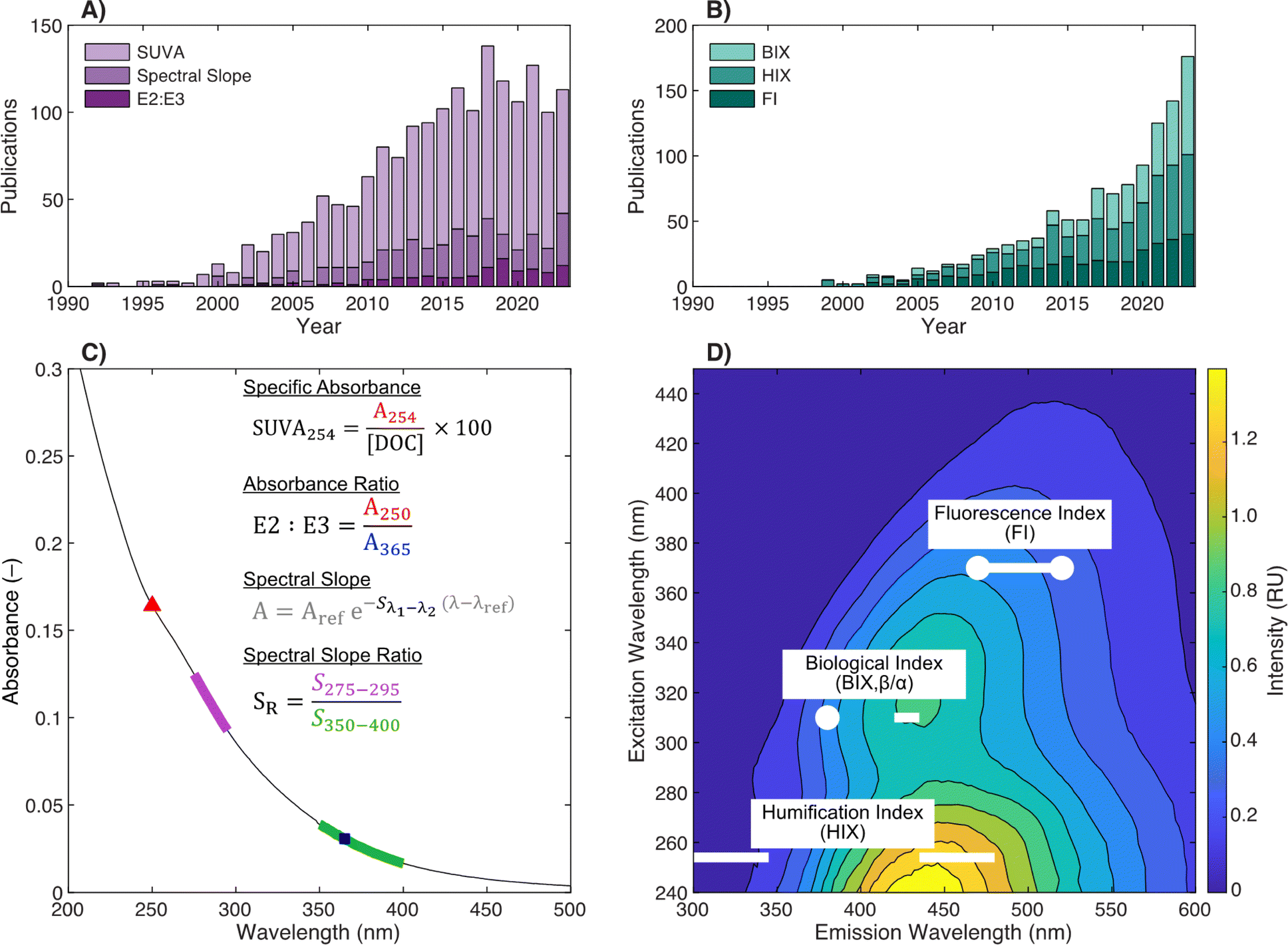 | ||
| Fig. 1 Overview of optical surrogates for characterizing dissolved organic matter (DOM). Annual number of publications referencing (A) absorbance- or (B) fluorescence-based surrogates in the indexed abstract. Details about search terms are in ESI Text 1.† Depictions of (C) absorbance- and (D) fluorescence-based surrogates. | ||
Despite their success and frequent use, optical surrogates are often not paired with independent measures of molecular weight and aromaticity, such as size exclusion chormatography (SEC) or nuclear magnetic resonance (NMR), respectively. This decision is understandable due to instrumental, sample, or cost limitations, but it leads to applying generalized interpretations in contexts different from the original studies in which physicochemical relationships were proposed. As a result, trends observed in one context are applied to explain results in another. Within DOM studies, changes in optical surrogates have been leveraged to explain qualitative changes in physicochemical characteristics, such as its photochemical reactivity26 or selective removal by coagulation.27 A quantitative example is applying regression models developed in other studies to report quantitative values for aromaticity and molecular weight in a new data set using only absorbance measurements.28 More broadly, interpretations derived from DOM samples in natural systems have been applied to different contexts without independent verification. Examples include treatment of highly specific feedstocks or anthropogenic waste streams29,30 and production of microplastic-derived organic matter.31,32 The lack of independent measures of DOM molecular weight and aromaticity in diverse contexts creates considerable uncertainty about interpretations derived from optical measurements, limiting progress in the field.
This critical review examines the foundation for optical surrogates commonly used to assess DOM molecular weight and aromaticity. For each surrogate, we review and scrutinize (1) the earliest known studies defining the surrogate and subsequent variations in definition that may be points of ambiguity in current literature, (2) the earliest known studies relating optical surrogates to aromaticity and/or molecular weight, (3) the experimental context for original studies (e.g., soil vs. water) that may constrain current interpretations, and (4) the continued inquiry into direct lines of independent evidence (e.g., NMR, membrane fractionation, SEC, etc.) for each surrogate. Although we focus the scope of this review on aquatic environments, many surrogates originated from soil science. We expect that this information will be useful to scientists and engineers studying DOM in aquatic systems and may serve as a framework for other environments, such as atmospheric aerosols.33,34
With respect to reviewing more recent, continued inquiry into optical surrogates, we focus on studies that (1) included a diverse range of source materials, (2) contrasted allochthonous and autochthonous endmembers, and (3) chemically characterized samples by multiple methods. Five papers are a consistent thread throughout the article due to data availability and breadth of organic matter sources.
First, Kellerman et al. (2018)35 presents optical surrogates paired with Fourier-transform ion cyclotron resonance mass spectrometry (FT-ICR MS) data from 37 isolates collected from diverse aquatic environments, representing arguably one of the strongest available datasets for this inquiry. Their samples were collected from aquatic systems and isolated using either reverse osmosis (RO) or XAD resin to produce natural organic matter (NOM), hydrophobic organic acid (HPOA), and fulvic acid (FA) fractions. Compared to the scope of this review article, all the optical surrogates discussed were published in the original paper with one exception. The original paper did not publish peak intensities or full excitation-emission matrices (EEMs). A fluorescence intensity was estimated by reconstructing intensities from decomposed parallel factor analysis (PARAFAC) components (ESI Text 4†). The measure of aromatic carbon in this paper was the relative abundance of formulae classified as condensed or polycyclic aromatic formulae as described in Section 2.3.2.
Two papers by Maizel and Remucal also characterized aromatic carbon using FT-ICR MS. Maizel and Remucal (2017)36 compared two endmember isolates, Suwannee River fulvic acid (SRFA) with Pony Lake fulvic acid (PLFA), and provided insight into molecular weight trends using ultrafiltration (UF) size fractionation. Another paper, Maizel and Remucal (2017),37 collected samples from seven different lakes in northern Wisconsin of diverse trophic status. Both papers interpreted FT-ICR MS data by calculating the double bond equivalents (DBE).38
The fourth paper is McKay et al. (2018)39 presenting optical surrogates from both aquatic and soil isolates, predominantly from the International Humic Substances Society (IHSS). These samples were paired with aromaticity data (13C NMR) from other primary sources.40–43 The last study, Mostafa et al. (2014),38 used UF to contrast two endmember samples: Suwannee River natural organic matter (SRNOM) and a secondary treated, wastewater effluent (EfOM).
Although measures of aromatic carbon derived from 13C NMR and FT-ICR MS are not directly comparable, both have become widely used methods to examine relationships between optical surrogates and aromatic carbon across diverse sources. Readers are referred to original sources for more details about study-specific instrumentation and methods. Lastly, many studies use IHSS isolates, and these materials have been isolated in different batches, each with a unique reference number. Readers are referred to original sources to determine if isolates presented across studies originated from the same batch.
Across the figures which synthesize data from multiple studies, several conventions are applied. In figures where correlations are calculated for literature data, the Spearman rank correlation coefficient (ρS) and associated p value (pS) are presented. This approach does not assume linearity between variables. If the original paper fit a non-linear model, these models are shown with the annotated equation (e.g., Fig. 4b). Least-squares linear regressions are shown selectively to highlight trends within a dataset. Regressions are not shown if rank correlations were not statistically significant (e.g., Fig. 4c, PLFA), or if generalized regressions would be suspect due to data clustering (e.g., Fig. 4c, Lakes). To include data from three literature sources,38,39,44 some surrogates were not calculated in the original study and were later calculated from spectra in the Korak and McKay (2024)45 meta-analysis; the original study that generated the data is attributed in the text and figures. Lastly, the conventional “et al.” is intentionally not printed in figure annotations due to space constraints; reference numbers are noted in the captions.
This review has three main Sections (2–4) followed by conclusions. Section 2 (background) presents some of the fundamental principles of absorbance and fluorescence spectroscopy, because some surrogates directly stem from these equations. Sections 3 and 4 cover absorbance and fluorescence surrogates, respectively. Within these sections, subsections focus on individual optical surrogates, detailing their genesis and exploring continued inquiry. These sections could be read in any order according to reader interest.
2 Background
In this section, terminology follows recommendations by the International Union of Pure and Applied Chemistry (IUPAC)46 unless otherwise specified. Generally, fundamental equations are presented for single compounds. DOM is a heterogeneous mixture, and the terms DOM and dissolved organic carbon (DOC) are often used interchangeably; distinctions are made when the context is specific to DOC concentration ([DOC]) measured on a carbon basis. Since not all DOM is optically active, compositional surrogates would be interpreted as “apparent” values for the mixture.2.1 Absorbance
Absorbance is the process by which a molecule absorbs light energy (i.e., photons). The energy required to promote an electron is determined by the energy difference between the ground and excited states, which is a function of the type of molecular orbital involved in the transition (n vs. π) and the presence of electron delocalization or conjugation.47,48 In DOM, absorbance in the ultraviolet-visible wavelength range (200–700 nm) primarily promotes π bond electrons associated with aromatic chromophores.49 The conjugation of the aromatic ring can be extended through the addition of electron withdrawing groups, like carbonyls, or electron donating groups, like hydroxy and alkoxy groups. Extended conjugation increases the absorbance maximum wavelength (lower energy transition) relative to benzene (Fig. 2a). Furthermore, extending the conjugation via fusion of two benzene rings, as in naphthalene, also results in lower energy transitions.51 The promotion of electrons associated with double bonds at 254 nm is why higher carbon-normalized absorbance is associated with higher aromaticity (Fig. 2b).50 In the visible wavelength range, chromophore identity is less clear but could originate from highly conjugated aromatics, charge-transfer interactions between aromatic moieties, or a combination of these two.49,52,53 | ||
| Fig. 2 (A) Molar extinction (ε, M−1 cm−1) spectra for model aromatic chromophores demonstrating the impacts of electron withdrawing groups (benzaldehyde, –CHO), donating groups (vanillin; –OH, –OCH3), and extended π conjugation on the energy of electronic transitions. The inset shows the spectrum of benzene. (B) Molar extinction spectra (ε, MC−1 cm−1) for DOM isolates from diverse sources with wide variations in aromaticity and specific ultraviolet absorbance at 254 nm (SUVA254). Spectra are from McKay et al. (2018)39 and paired with 13C NMR data from other sources.40,50 Samples include Pahokee Peat Fulvic Acid (PPFA), Mississippi River Natural Organic Matter (MRNOM), and Pacific Ocean Fulvic Acid (POFA). | ||
Quantitatively, absorbance is defined as the ratio of incident (P0λ) to radiant (Pλ ) spectral power at a specific wavelength (λ) (eqn (1)). The Bouguer–Beer–Lambert law relates absorbance to concentration (c) and pathlength
  using a proportionality constant (ε or κ). Depending on the logarithm convention, calculations using a base 10 logarithm pairs the terms absorbance (A(λ)) and molar decadic absorption coefficient (ε) following eqn (1). Calculations using the natural logarithm pair the terms Napierian absorbance (Ae(λ)) and molar Napierian absorption coefficient (κ) following eqn (2). Formal derivations are summarized elsewhere.54,55 The molar absorption coefficients κ and ε are related through eqn (3).
 | (1) |
 | (2) |
| κ = 2.303ε | (3) |
Differentiating these conventions is important for calculating DOM optical surrogates.56 For example, decadic absorbance (A(λ)) is commonly used to calculate SUVA, whereas spectral slope calculations fit regressions to linear Napierian absorption coefficients (α = κc). Note, the DOM community commonly uses the acronym a for the linear Napierian absorption coefficient,57 which is inconsistent with current IUPAC conventions.46 Decadic absorption coefficients (ε) are commonly reported for freshwaters, whereas the marine community typically reports Napierian absorption coefficients.
DOM is generally assumed to follow the Bouguer–Beer–Lambert law across environmentally relevant concentrations.58,59 For dilution series, non-zero intercepts indicate the contribution of non-chromophoric carbon. The effects of the cuvette or solvent are eliminated by pairing measurements with a reference cell through either a double beam configuration or subtracting a blank spectrum. To measure absorbance at ultraviolet wavelengths, a cuvette material with high transmittance (e.g., quartz) is necessary.
The Bouguer–Beer–Lambert law only describes absorbance – not attenuance due to light scattering by suspended particles. Although also measured on a spectrophotometer, attenuance is a function of both absorbance and light scattering. Isolating the absorbance phenomenon requires sample filtration. For absorbance measurements alone (not fluorescence), regulatory methods (e.g., Standard Method 5310 or USEPA 415.3)60,61 often define the dissolved fraction as <0.45 μm using a range of organic-based materials (e.g., nylon, polyethersulfone). These filters have low potential to adsorb DOM or leach material that interferes at 254 nm after sufficient rinsing.62 Across the research community, selection of filter material and nominal pore size (e.g., 0.2–0.7 μm) is highly variable. This distinction between absorbance and attenuance is particularly important for online sensor data.
2.2 Fluorescence
Generated by light absorbance, singlet excited states can return to the ground state (called S0) through several different pathways, one of which is fluorescence. Initially, excited molecules undergo relaxation to the lowest vibrational level of the first singlet excited state (called S1),63 and fluorescence occurs from this state when the excited molecule emits a photon with an energy (∝ wavelength−1) corresponding to the energy gap between S1 and S0. Fluorescence always occurs at emission wavelengths longer than the excitation/absorbance wavelength due to the energy lost during relaxation of the singlet excited state via vibrations and solvent reorientation, which is called the Stokes Shift.54,64 In addition to fluorescence, relaxation from S1 to S0 can occur through non-radiative pathways such as internal conversion (IC) and intersystem crossing (ISC) to a triplet state (e.g., T1). From the triplet state, relaxation can occur through radiative (i.e., phosphorescence) or non-radiative IC processes. The fluorescence quantum yield (Φf) is the ratio of the fluorescence rate constant (kf) relative to the sum of the rate constants for radiative and nonradiative (knr) decay pathways (eqn (4)).54,65 | (4) |
An analogous quantum yield can be defined for relating ISC to a triplet state to other pathways.46,65 For DOM, fluorescence quantum yields39,66,67 are typically ∼1%, and ISC quantum yields68 are ∼5%, suggesting that most photons absorbed by DOM are lost through non-fluorescence pathways. Although DOM fluorescence studies have taken advantage of both time-resolved and steady-state methods,69–72 we focus here on steady-state methods used to calculate optical surrogates.
Benchtop spectrofluorometers use narrow slits to focus semi-monochromatic light on a narrow cross section of the cuvette. Emitted light is measured from a small interrogation zone perpendicular to the incident light (Fig. 3). Following derivations published elsewhere,73,74 fluorescence intensity (If) is proportional to Φf and the power of light absorbed (Pλ(x1) − Pλ(x2)) across the interrogation zone (eqn (5)). Applying the Bouguer–Beer–Lambert law across the interrogation zone, Iλ is not proportional to concentration. Note, this source of non-linearity is different from inner filter effects (vide infra).
| Iλ = Φf(Pλ(x1) − Pλ(x2)) = ΦfPλ(x1)(1 − e−κcΔx) | (5) |
 | ||
| Fig. 3 Schematic of the cross-section (top view) of a square cuvette with annotated dimensions used in fundamental equation derivations. | ||
However, in practice, a linear relationship between Iλ and c is commonly observed and is an underlying assumption for many intrinsic fluorescence surrogates (e.g., ratio of fluorescence intensities or [DOC]-normalized fluorescence intensity).75–77 A linear relationship between fluorescence intensity and concentration is supported mathematically by applying a power series expansion (eqn (6)) and assuming absorbance across the interrogation zone (Δx) is small. This approximation simplifies eqn (5) to (7). In practice, regressions between [DOC] and fluorescence intensity often have a non-zero intercept due to non-fluorescent DOM.75,76
 | (6) |
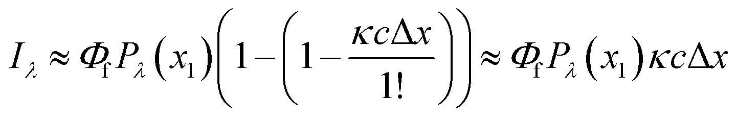 | (7) |
The practical application of eqn (7) requires fluorescence measurements that are free of instrumental or other optical artifacts. Like absorbance, filtration prevents light attenuation due to suspended particles. For fluorescence, glass fiber filters (GF/F) are commonly used with a nominal pore size 0.7 μm. Although GF/F filters have a lower potential to leach fluorescent material, they still need to be muffled and thoroughly rinsed to remove any binding material.78 Notably, the common choice of GF/F filters for fluorescence conflicts with the 0.45 μm cut-off specified in USEPA method 415.3 for absorbance.60 Within the DOM field, Murphy et al. (2010)79 outlines the broadly accepted fluorescence correction procedures.58 These corrections include instrument-specific correction factors, blank subtraction, scatter masking, intensity normalization, and inner filter corrections. Software packages that perform these corrections are available in MATLAB,80,81 R,82 and proprietary software (e.g., Horiba's Aqualog). Instrument-specific correction factors are unique to each spectrofluorometer and are often provided by manufacturers to account for wavelength-specific efficiencies of light transmission.83,84 Blank subtraction, like absorbance reference cells, isolates the sample fluorescence independent of the solvent and cuvette. Blank subtraction is partially effective to remove Rayleigh and Raman scattering, but most analyses excise and interpolate scatter.80,81,85,86 Finally, signal normalization scales the intensities by either the integrated area of the Raman peak for deionized water (Raman Units; RU) or the emission from a model fluorophore like quinine sulfate (Quinine Sulfate Units; QSU).87,88
Inner filter corrections account for light absorbance to and from the interrogation zone (Fig. 3). Primary inner filtering is the loss of light between the incident cuvette edge and the interrogation zone. Secondary inner filtering is the loss of emitted light between the interrogation zone and the cuvette edge perpendicular to the incident light. Inner filter corrections apply broadly across fluorescence spectroscopy, and several studies have proposed or derived correction procedures over the past 60 years using absorbance-based approaches,59,89–95 controlled dilution approaches,59,96 and cell shift methods.89,97 The latter two approaches are less common in the DOM community; readers are referred to the cited references for more details. The absorbance-based approach is the most common correction following eqn (8). The correction factor is a function of the sum of (decadic) absorbance values at the excitation (A(λex)) and emission wavelengths (A(λem)), assuming the same pathlength for fluorescence and absorbance spectroscopy. If absorbance and fluorescence measurements use different pathlengths, absorbance must be normalized to the fluorescence pathlength before applying eqn (8). Kothawala et al. (2013) reported that eqn (8) performed sufficiently up to an absorbance sum of 1.5.59
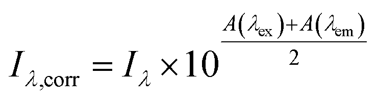 | (8) |
To illustrate the magnitude of corrections, consider a scenario where A(λex) is 0.1 and A(λem) is 0.05 making the absorbance sum 0.15. The observed fluorescence intensity (Iλ) would be corrected by multiplying it by a factor of 1.19. If uncorrected, the observed fluorescence would be 19% too low due to inner filtering (Fig. S1†). Some studies cite a DOC concentration threshold to justify the need for inner filter corrections (or lack thereof). This approach is strongly discouraged, because inner filter effects are an absorbance-based phenomenon. A DOC concentration criterium would assume all DOM has the same absorbance per unit carbon.59
Although broadly used, the derivation of eqn (8) includes some simplifying assumptions that may not be appropriate in all cases. Similar to the linearization of eqn (5), inner filter corrections also use a power-series expansion (eqn (6)), which assumes the quantity κcΔx is small, to linearize an exponential term. The second assumption is that the interrogation zone is in the middle of cuvette  . The application of eqn (8) on benchtop spectrofluorometers is generally appropriate. Kubista et al. (1994) showed that quantifying the interrogation zone size is not important for most practical applications, and the same empirical correction equation could be used for bandpasses between 0.5 and 15 nm.91 However, adaptation of benchtop methods to other applications, such as field sensors, may need to reevaluate these assumptions. Full derivations are provided elsewhere.90,92,98
Spectrofluorometers from many manufacturers have been used by the DOM research community, including Aminco-Bowman, PerkinElmer, Varian, and Horiba. Small but meaningful differences in fluorescence spectra have been documented and would be expected between different spectrofluorometers given differences in hardware.79 Even within Horiba instruments, substantive instrument bias has been reported between the Aqualog and Fluoromax (e.g., F3 and F4), which, in part, results from differences between excitation gratings in the Fluoromax-4 (plane ruled), that passes more stray light, compared to the Aqualog (concave holographic).99 Past research has shown that apparent quantum yields at excitation wavelengths less than 350 nm are systematically larger on the Fluoromax-4 compared to the Aqualog.39 Unfortunately, the impact of these instrument biases on fluorescence-derived optical surrogates are not well-constrained in the DOM research community. In contrast, fluorescence-based surrogates that rely on intensity ratios at the same excitation wavelength may be less impacted.
2.3 Estimation of DOM molecular weight and aromaticity
UF fractionated samples yield categorical molecular weight classifications (e.g., <1 kDa, 1–3 kDa, >3 kDa). Each filter has a nominal molecular weight cutoff, but two filters with the same nominal cut-off may perform differently due to membrane surface chemistry, DOM concentration, and aqueous ionic composition.115,116 GPC, without the use of a high-pressure pump, was commonly used in many early papers by packing columns with Sephadex resins of different pore sizes.103,104 To decrease sample volumes and increase resolution, high-pressure SEC uses macroporous resins with online detectors.106,117,118 In both GPC and SEC, smaller molecules are retained in the column and elute after longer times compared to larger molecules. The detector signal can be numerically integrated across the SEC chromatogram to calculate either a number-average (Mn) and weight-average (Mw) molecular weight. Polydispersity (Mw/Mn) is generally greater than unity for DOM, implying that Mw is greater than Mn.
For FT-ICR MS, ions are detected, and formulae are assigned based on the accurate mass using automated programming algorithms and a set of rules.133 FT-ICR MS has both instrumental limitations, where ion detection may be biased to low molecular weights,135 and data analysis limitations, where unambiguous formula assignment is often limited to mass-to-charge ratios (m/z) between 150–1000.132,133,140 Using the assigned formulae, metrics can be calculated, such as modified aromaticity index (AImod)132 and double bond equivalents (DBE).141 These metrics are used to group assigned molecular formulae into chemical characterization categories that suggest aromatic or condensed aromatic moieties in the DOM samples. Mass spectral peak intensity-weighted averages, based on all assigned formulae in a sample, are also reported. For example, Kellerman et al. (2018)35 used AImod132 based on FT-ICR MS data to calculate relative abundance (%) of two classes: condensed or polycyclic aromatic formulae (AImod > 0.66) and polyphenolic formulae (0.66 ≥ AImod > 0.5) using the formula bounds of C1–45H1–92N0–4O1–25S0−2.
Estimates of aromaticity are not directly comparable when derived using different instrumental (e.g., NMR or FT-ICR MS) or calculation methods (e.g., AImod boundary conditions). NMR probes all 13C carbons, albeit at different shifts depending on chemical environment. For example, considering two structural isomers, cyclohexane and hexene (each having one degree of unsaturation), hexene would have a 13C resonance at about 120 ppm (from the sp2 hybridized carbon), whereas cyclohexane would have only aliphatic carbon resonances <60 ppm.141 In contrast to NMR, FT-ICR MS only detects molecules that can be ionized (in either positive or negative ion mode) and characterized as having aromatic nature, subject to meeting signal-to-noise thresholds.132,142 Past work suggests that UV chromophoric DOM is poorly ionized by negative mode electrospray ionization143 and is therefore poorly represented in the majority of studies characterizing the chemical nature of DOM with ultra-high resolution mass spectrometry techniques. In contrast, a study by Laszakovits et al. (2020) demonstrated that a higher percent of assigned formulae were characterized as aromatic and condensed aromatic using laser desorption ionization (in both positive and negative mode) compared to electrospray ionization.144 For future inquiries relating optical surrogates to composition, there is an opportunity to explore multiple ionization techniques.
In this review, FT-ICR MS is considered as a technique to assess the abundance of aromatic carbon, despite its limitations, due to its growing popularity in DOM research.145 FT-ICR MS data has also been analyzed to calculate molecular weight distributions of DOM146,147 but will not be used as a comparison measure in this review. Due to incomplete DOM recovery by SPE148–151 and limitations of the analytical mass range132,133,140 and ionization efficiency,131,144,152 values derived from FT-ICR MS data are far from comparable to other methods that characterize molecular weight. This review focuses on UF and SEC to characterize molecular weight.
Overall, all characterization methods for molecular weight and aromatic carbon are subject to sampling, analytical, and methodological constraints. Readers are referred to primary sources for details about sample preparation, instrument biases, method background and limitations, and other challenges with DOM chemical characterization.
3 Absorbance surrogates
Absorbance-based optical surrogates are listed in Table 1 along with the equations and primary sources. The following subsections explore each surrogate.| Metric | Examples | Calculation | Units | Notes | References |
|---|---|---|---|---|---|
| Specific absorbance | SUVA254 |

|
L mgC−1 m−1 | λ: wavelength of incident light | Traina et al. (1990)153Chin et al. (1994)154Peuravuori and Pihlaja (1997)155Weishaar et al. (2003)50 |
| SUVA280 | A λ : decadic absorbance at λ normalized to a pathlength of 1 cm | ||||
| SUVA300 | [DOC]: dissolved organic carbon concentration | ||||
| Absorbance ratio | E2![[thin space (1/6-em)]](https://www.rsc.org/images/entities/char_2009.gif) :E3 :E3 |

|
— | A 250nm: decadic absorbance at 250 nm | De Haan (1972)156 |
| A 365nm: decadic absorbance at 365 nm | Peuravuori and Pihlaja (1997)155 | ||||
| E4:E6 |

|
— | A 465nm: decadic absorbance at 465 nm | Chen et al. (1977)157 | |
| A 665nm: decadic absorbance at 665 nm | |||||
| Spectral slope (non-linear) | S 300–600 |

|
nm−1 | S λ 1−λ2: spectral slope between λ1 and λ2 | Stedmon et al. (2000)158 |
| S 300–650 | Kowalczuk et al. (2005)159 | ||||
| S 300–700 | λ ref: reference wavelength, typically 350 nm | Twardowski et al. (2004)160 | |||
| Helms et al. (2008)57 | |||||
| Spectral slope (linear) | S 275–295 |

|
nm−1 | b is the intercept (typically not reported) | Helms et al. (2008, 2013)57,161 |
| S 350–400 | Fichot and Benner (2012)162 | ||||
| Spectral slope ratio | S R |

|
— | Helms et al. (2008)57 |
3.1 Specific absorbance
Since specific absorbance is an application of the Bouguer–Beer–Lambert law, the genesis within DOM research dates to the earliest inquiries. Juday and Birge (1933)3 explored specific absorbance indirectly by plotting color (in platinum-cobalt units) versus DOC concentration, showing a correlation for >500 lakes in Wisconsin (USA). Later, James (1941)58 diluted lake samples, calculated a “molecular absorption coefficient”, and showed agreement with the Bouguer–Beer–Lambert law for up to a 20-fold dilution across 5 visible wavelengths (407.9 to 700 nm). Over the following decades, most studies commonly reported color per unit carbon for individual samples or the slope of a linear regression between color and DOC concentration for multiple samples.2,105,122,163–166 For example, Packham (1964) reported that the specific absorbance for humic acid (HA) isolates was greater than paired the fulvic acids for 7 samples at 300 and 450 nm.165
Specific absorbance has been reported at wavelengths spanning the ultraviolet50,154,167,168 and visible regions,121,169–171 with early studies mostly reporting visible wavelengths and more recent studies focusing on ultraviolet wavelengths. Ghassemi and Christman (1968)169 fractionated samples with Sephadex and noted higher absorbance per unit carbon at 350 nm in the larger molecular weight fractions. Despite a 1953 study which advocated for monitoring at 275 nm,172 254 nm gained popularity in the 1960s and 1970s due to this wavelength aligning with an emission maxima of low-pressure mercury lamps.173–176 Focus shifted from using absorbance as a surrogate for DOC concentration to using specific absorbance as an intrinsic surrogate of DOM composition. Studies demonstrated relationships with coagulation efficiency14 and disinfection byproduct formation using both the color-to-[DOC] ratio in 1983 (ref. 177) and then SUVA254 in 1985.15 Although independent measures of molecular weight or aromaticity were not the focus of these early studies, the context for measuring UV absorbance was consistently framed as probing the π→π* transitions occurring in O- and N-substituted aromatic compounds such as phenols.15,173,174,178,179 However, some early studies also correlated specific absorbance to molecular weight121,180 or qualitatively described the UV absorbance as dependent on both chemical characteristics181 (and not mutually exclusive).
3.1.2.1 Aromaticity. Like many optical surrogates, early explorations of aromaticity are rooted in soil humic substances. Traina et al. (1990)153 correlated 13C aromaticity with SUVA272 for humic substances extracted from soil, showing good agreement with data for humic substances extracted from marine sediments and terrestrial soils from Gauthier et al. (1987).179 For the combined dataset, the linear regression was strong (n = 12, r = 0.937),153 but as a note of caution, absorbance was normalized to the material mass, not carbon mass, which may underestimate specific absorbance due to residual water and ash.
Transitioning to aquatic DOM, Chin et al. (1994)154 studied the relationship between SUVA280 and both 13C aromaticity and molecular weight for aquatic fulvic acids, presenting a strong positive correlation between SUVA280 and 13C aromaticity spanning autochthonous and allochthonous sources (Fig. 4a). Similarly, SUVA300 and 13C aromaticity were positively correlated in McKnight et al. (1997)182 for fulvic acids from diverse origins, including the Suwannee River, two Antarctic lakes (Pony Lake and Lake Fryxell), and an alpine watershed in Colorado (USA). Notably, the coefficient of determination (R2) for the regression with 13C aromaticity was stronger for SUVA300 (R2 = 0.76) than SUVA450 (R2 = 0.43). Croue et al. (2000)125 fractionated four waters using RO and XAD resins, also affirming a positive correlation between SUVA254 and 13C aromaticity (R2 = 0.72, n = 27). Currently, the highest cited paper relating SUVA254 to 13C aromaticity is Weishaar et al. (2003),50 which included fulvic acid-dominated isolates from diverse aquatic origins ranging from the Pacific Ocean to the Florida Everglades (13C aromaticity (%) = 6.52 × SUVA254, n = 13, R2 = 0.97) (Fig. 4a). Pairing the specific absorbance data from McKay et al. (2018)39 with 13C data from other studies,40–43 there is continuity in the correlation for the sample set expanded to include an aquatic humic acid and three soil isolates, which is not be the case for some other surrogates (vide infra).
 | ||
| Fig. 4 Relationship between specific ultraviolet absorbance (SUVA) and either molecular weight or different measures of aromatic carbon. (A) SUVA254 and SUVA280versus aromaticity (%) per sample calculated from 13C NMR data.39–43,50,154 (B) SUVA254versus the relative abundance of condensed aromatic and polyphenolic formulae (%) per sample calculated based on AImod132 from FT-ICR MS data.35 (C) SUVA254versus average double bond equivalents (DBE) calculated based on FT-ICR MS data for size-fractionated fulvic acid isolates (PLFA and SRFA)36 and seven different lakes in northern Wisconsin of diverse trophic status.37 (D) SUVA280versus number-average (Mn) and weight-average (Mw) molecular weight determined by SEC with UV detection.154 (E) Number-average molecular weight versus SUVA280 for SEC with UV detection.155 (F) SUVA254versus UF molecular weight fraction for three isolates (SRFA, PLFA, and SRNOM) and effluent organic matter (EfOM).36,38 | ||
More recently, molecular formulae assigned using FT-ICR MS data were analyzed to characterize differences in aromatic carbon. For DOM samples from the Florida Everglades, molecular formulae with lower hydrogen-to-carbon (H/C) ratios (higher DBE) correlated positively with SUVA254.183 In Maizel and Remucal (2017),36 increases in DBE were associated with increases in SUVA254 between two clusters of lakes in Wisconsin of diverse trophic status (Fig. 4c). Encompassing the broadest set of NOM, HPOA, and fulvic acid isolates (SUVA254 0.6–4.9 L mgC−1 m−1), Kellerman et al. (2018) reported an exponential relationship between SUVA254 and the relative abundance of condensed aromatic and polyphenolic formulae (Fig. 4b).35
3.1.2.2 Molecular weight. The contemporary understanding for DOM is that SUVA increases as molecular weight increases, although some early studies proposed the opposite.101,184 Utilizing cultures from soil-derived microorganisms (actinomycetes), Ewald et al. (1988)180 fractionated DOM using XAD-2 resin185 and UF (500 and 100
000 Da) followed by pH adjustment to 2 and 13. For the UF fractions, molar absorption coefficients at 370 nm (ε370) increased proportionally to the log of the molecular weight with higher ε370 values at pH 13 than pH 2.180 Contrasting a Nordic lake with rivers in southeastern USA, Alberts and colleagues186,187 fractionated samples by UF, characterized the fractions by SEC (DOC and UV254 detectors), and confirmed increasing SUVA254 with increasing molecular weight. More recently, Mostafa et al. (2014)38 and Maizel and Remucal (2017)36 fractionated endmember aquatic DOM samples with UF, also affirming increased SUVA254 with increasing nominal filter cutoffs for most isolates (Fig. 4f). Notably, UF fractionated EfOM did not show a dependence of SUVA254 on molecular weight.
Use of specific absorbance to interpret aromaticity and molecular weight as independent characteristics is limited, because they correlate with one another. Both Chin et al. (1994)154 and Peuravuori and Pihlaja (1997)155 reported a positive correlation between SUVA280 and both 13C aromaticity and number-average molecular weight (Mn) (Fig. 4a, d and e). Maizel and Remucal (2017)36 fractionated SRFA with UF and used FT-ICR MS to show average DBE increased with increasing molecular weight, both correlating with SUVA254 (Fig. 4C). However, size-fractioned PLFA did not exhibit the same internally consistent relationship between DBE and SUVA254. Despite these correlated relationships, one cannot assume that high molecular weight DOM will also have high SUVA254; large biopolymers, like polysaccharides, that are abundant in EfOM often have low molar absorption coefficients.117,118
Taken as a whole, both historical and more recent literature support that SUVA generally increases with both molecular weight and aromaticity across samples from diverse geographic sources, but microbial endmembers may deviate from this generalization. In addition, asserting that SUVA is unique to aromaticity and not molecular weight is inconsistent with the frequent correlation of these characteristics reported in the primary literature.
3.2 E2:E3
The genesis of E2:E3 appears in De Haan (1972),156 although several earlier papers used absorbance ratios at different excitation wavelengths (see the Spectral Slope Section 3.4). De Haan (1972) concentrated samples from “shallow peaty lakes” in the Netherlands using pH adjustment (pH 7.0), decalcification (ion exchange), and freeze drying. The freeze-dried samples were reconstituted and fractionated by Sephadex size exclusion resin (G-25) measuring the absorbance at 250 nm semi-continuously. Sephadex G-25 produced three chromatographically resolved fractions (I, II, and III). Fig. 5d illustrates the correlation between the whole-water E2:E3 (pH 7.0) and the percentage of low molecular weight material (fraction III) from the freeze-dried, decalcified sample. Compared to the lower molecular weight fraction, correlations were weaker between E2:E3 and the percentage of either medium (II) or high (I) molecular weight DOM.46
 | ||
| Fig. 5 Relationship between E2:E3 (A250/A365) and either molecular weight or different measures of aromatic carbon. (A) E2:E3 versus aromaticity (%) per sample calculated from 13C NMR data.39–43,155 (B) E2:E3 versus the relative abundance of condensed aromatic and polyphenolic formulae (%) per sample calculated based on AImod132 from FT-ICR MS data.35 (C) E2:E3 versus average double bond equivalents (DBE) calculated based on FT-ICR MS data for UF fractionated isolates (PLFA and SRFA)36 and seven different lakes in northern Wisconsin of diverse trophic status.37 (D) E2:E3 of the whole-water versus the percentage of low molecular weight DOM (longest retention time) for a lake.156. (E) E2:E3 versus number-average molecular weight (Mn) for DOM from Nordic surface waters (humic substances and ultrafiltered samples).155,188 (F) E2:E3 versus nominal molecular weight fractions for endmembers following UF fractionation.36,38 | ||
Two later papers by De Haan and co-workers77,189 are often cited to support the inference of DOM molecular weight from E2:E3 measurements. First, De Haan et al. (1983)189 measured E2:E3 for a ditch water sample derived from peat soil drainage at pH values between 2.0 and 10.5. Compared to pH 2, the relative change in absorbance ([ApHX − ApH2]/ApH2 × 100) increased by over 30% from pH 2 to 10.5 at 365 nm, whereas the increase was only about 5% at 250 nm. Therefore, E2:E3 decreased with increasing pH. Furthermore, the ditch water DOM was fractionated using dialysis and UF to assess the molecular weight distribution of chromophoric DOM as measured by absorbance spectroscopy. Increasing the pH decreased the relative fraction of chromophoric DOM that permeated through a 25 Å cutoff dialysis bag. The relative fraction was positively correlated to the peak area of the highest molecular weight fraction separated by Sephadex G-25, corroborating the dialysis measurements. In addition, for ultrafilters of a given pore size (between 50 and 150 Å), a larger fraction of chromophoric DOM was retained as pH increased from 3 to 7, also consistent with the dialysis results. Based on these observations and prior work,156 De Haan et al. (1983)189 concluded that the, “decrease of E250/E365 with increasing pH indicated increasing molecular weight and size of the fulvic acid with increasing pH” (page 71, paragraph two). The second study, De Haan and De Boer (1987),77 reported that E2:E3 increased with smaller membrane cutoffs for 38 UF fractionations from a single lake (Fig. 5b).
To summarize, the genesis of E2:E3 as a surrogate for DOM molecular weight is based on individual DOM samples subjected to molecular weight fractionation or pH titration. This surrogate was not developed to compare DOM from multiple geographic sites with independent molecular weight distributions. In practice, E2:E3 is often interpreted with specificity for molecular weight. However, another early study by De Haan (1983) complicates this interpretation, because curie point pyrolysis/mass spectrometry showed that increased molecular weight coincides with increased aromatic compounds (i.e., phenols) and decreased E2:E3 ratios.190
3.2.2.1 Molecular weight and aromaticity. Since the original work of De Haan and colleagues, Peuravuori and Pihlaja (1997, 2004)155,188 are cornerstones for generalized interpretations of E2:E3 for DOM molecular weight and aromaticity. Peuravuori and Pihlaja (1997)155 evaluated the relationships between molecular weight (by SEC) and aromaticity (by 13C NMR) with both SUVA280 (L molC−1 cm−1) and E2:E3 for lake samples (n = 2), river water (n = 1), and many (n > 60) isolates derived from these three whole-water samples (see Section 3.1 for SUVA280 discussion). Humic acid, fulvic acid, and hydrophobic neutral fractions were isolated using an XAD-8 procedure.191 In addition, each whole-water was ultrafiltered using membranes with various nominal molecular weight cutoffs (NMW, in Da) into three fractions (I, NMW>100
000; II, NMW 10,000–100,000; III, NMW 1000–10000). Each UF fraction was further subjected to three further treatments: freeze-drying, cation exchange followed by freeze-drying again, followed by XAD-8 isolation of humic- and fulvic acid fractions from the UF fractions. Finally, selected samples were ultrafiltered to obtain an NMW <1000 fraction (IV) followed by XAD-8 isolation.
Peuravuori and Pihlaja (1997)155 presented single parameter regressions using E2:E3 as a predictor of either aromaticity using XAD isolates (eqn (9), linear) or Mn using UF fractionated samples (eqn (10), semilog).
| Aromaticity (%) = 52.059 − 6.780 × E2:E3, n = 39, R2 = 0.78 | (9) |
| logMn = 5.341 − 0.401 × E2:E3, n = 40, R2 = 0.70. | (10) |
The regressions used a subset (n = 39 or 40) of the total sample set (n > 60), because the authors excluded UF samples that were further treated by freeze drying alone or freeze drying after calcium removal by ion exchange. Thus, the sample context at the core of these regressions is limited to hydrophobic acids and hydrophobic neutrals.
Peuravuori and Pihlaja (2004)188 used preparative scale SEC to separate DOM into eight molecular weight fractions. The sample context was Lake Savojäri (southwestern Finland), a marsh containing ∼20 mgC L−1. Fig. 5e shows that there is an exponential relationship between E2:E3 and Mn for the 2004 dataset, agreeing with the general trend from the 1997 study.155 Unfortunately, aromaticity was not reported in this later study. In both studies, E2:E3 values have a lower limit of ∼3, even for the highest molecular weight fractions.155,188
More recently, two studies used UF to fractionate endmember samples (i.e., PLFA and SRFA).36,39 For both microbial and terrestrial endmembers, there were internally consistent trends for each sample; E2:E3 increased as molecular weight decreased (Fig. 5f).
3.2.2.2 Aromaticity. Using FT-ICR MS, Kellerman et al. (2018) applied nonmetric multidimensional scaling to show that DOM molecular formulae associated with aliphatic and less aromatic chemical species typically had higher E2:E3 values.35Fig. 5b shows an inverse correlation between E2:E3 and the relative abundance of condensed aromatic and polyphenolic formulae (ρs = −0.83, ps < 0.05). Although statistically significant, the data are more scattered as aromaticity decreased. For example, isolates with condensed aromatic and polyphenolic formulae > 30% consistently have low E2:E3 values (∼5), while samples with the lowest formula abundance (<10%) have E2:E3 values that span the dataset range.35
Also using FT-ICR MS, Maizel and Remucal (2017)36 compared DOM molecular formulae to E2:E3 for lakes of diverse trophic status. Of formulae assigned across all samples, 97% of those formulae that correlated positively with E2:E3 had a greater relative intensity in oligotrophic lakes. These formulae were also more oxidized and aliphatic than the 452 formulae that correlated negatively with E2:E3,36 consistent with Kellerman et al. (2018).35Fig. 5c shows that size-fractioned SRFA exhibited an inverse correlation between E2:E3 and average DBE with borderline statistical significance. Lake samples clustered into 2 groups where samples with higher E2:E3 had lower average DBE. However, the size-fractionated microbial endmember, PLFA, showed no systematic trend between these same variables. Lastly, Fig. 5a overlays the optical data from McKay et al. (2018)39 to show both general agreement with Peuravuori and Pihlaja (1997)155 and continuity of the correlation with three soil isolates having 13C aromaticity >35%. However, there was no statistically significant correlation across a subset including only the aquatic HPOA, NOM, and fulvic acid isolates (ps = 0.3, aromaticity <25%).
Collectively, this review highlights that the foundation for relating E2:E3 to molecular weight hinges on a few samples that have been fractionated or isolated to reveal trends that are internally consistent. Particularly for molecular weight, without a breadth of samples across different spatiotemporal scales, E2:E3 may be better suited for examining changes across natural or engineered treatment gradients for a single sample or samples related closely in origin. In future assessments of broader sample contexts, it is imperative to keep pH constant between samples when measuring E2:E3, as the pH dependence of E2:E3 served as one of the earliest citations189 to the dependence of this surrogate on molecular size. Even though the effects of pH were evaluated in the E2:E3 genesis papers, pH may impact both absorbance- and fluorescence-based surrogates more broadly,21,192–197 and there is a general need to standardize pH adjustment practices across the DOM research field.
3.3 E4:E6
For aromaticity, Kononova (1966)206 postulated that E4:E6 is a surrogate for the degree of condensation of “aromatic nets of carbon atoms” in soil humic acids. The position recognized that E4:E6 was higher for fulvic acids than humic acids. Within humic acids, E4:E6 decreased from podzolic soils to chernozems, which is associated with a simultaneous decrease in aliphatic side chains.206 This logic was later refuted in Chen et al. (1977)157 but applied by Ghosh and Schnitzer (1979)207 to describe macromolecular characteristics with changing pH and ionic strength.
Two studies investigated the relationship between E4:E6 and molecular weight using Sephadex gels. Tan and Giddens (1972)200 characterized poultry litter, sewage sludge, and loamy sand, and Chen et al. (1977)157 characterized soils from a range of classifications. Both studies reported lower E4:E6 ratios for humic acids than fulvic acids and an inverse correlation between molecular weight and E4:E6.157,200 In Tan and Giddens (1972),200 E4:E6 correlated positively with the Sephadex G-50 partition coefficients for fulvic acids, but a similar relationship was not observed for humic acids.200 For size-fractionated soil isolates, Chen et al. (1977) reported significant correlations between E4:E6 and several physicochemical properties, including reduced viscosity (r = −0.95 a measure of molecular size), % carbon (r = −0.73), % oxygen (r = 0.82), total acidity (r = 0.62), and carboxyl content (r = 0.66).157 The same study explored the relationship between E4:E6 and Mw as a function of pH, similar to the approach used by De Haan et al. (1983)189 between E2:E3 and Mn for aquatic DOM. However, the pH-dependence of E4:E6 (soil isolates) and E2:E3 (aquatic isolates) was opposite. For soils, E4:E6 increased with increasing pH (from 2 to 7) with concomitant increases in Mw,157 whereas E2:E3 decreased with increasing pH for aquatic DOM even though Mn increased.189 In the end, Chen et al. (1977) argued that E4:E6 is a better indicator of molecular weight than of the abundance of condensed aromatic rings.157
3.4 Spectral slopes and the spectral slope ratio
Interestingly, the earliest references to use the term “spectral slope” describe what today would be called an absorbance ratio. For example, Packham (1964) reports that the absorbance ratio of 300 to 450 nm is greater for fulvic acids than paired humic acids across 7 samples.165 Kalle (1966) compared spectral steepness for marine DOM using an absorbance ratio of 420 to 665 nm.216 Similarly, Brown (1977) defined spectral slope as the ratio of 280 to 310 nm.217 Thus, absorbance ratios like E2:E3 are historically a spectral slope.
One of the first studies to use >2 wavelengths was Kopelevich and Burkenov (1977), in which log-transformed data was fit using a linear regression between 390 and 490 nm.215 In early studies, S was leveraged as both a characterization tool, focusing on variability between samples, and as a modeling tool, assuming little variability between samples. Often cited in later key studies,57,160,218 Zepp and Schlotzhauer (1981)67 characterized spectral slopes between 300 and 500 nm noting similar values (range 0.0128–0.0175 nm−1) for soil fulvic acids and DOM from freshwater and marine environments (linearization not specified). Bricaud et al. (1981) advocated that the small variability between samples would enable an average value of S to be used to extrapolate absorbance spectra from the UV range (375 nm) to the visible range (440 nm).213 Blough and coworkers used spectral slopes, calculated from log-transformed data, to characterize differences in water samples from the Orinoco River outflow,219 Gulf of Mexico,220 and Amazon River.220 With linearization, however, absorbance near or below detection disproportionately impacts fitted model parameters. To minimize impacts, Blough, Green, and coworkers219,220 defined a detection limit (absorption coefficient = 0.1 m−1) and fit linear regressions for sample-specific wavelength ranges where absorbance exceeded the limit.
These examples highlight the challenges in comparing spectral slopes between studies that arise due to differences in wavelength range and regression technique. Twardowski et al. (2004) recognized and addressed this issue comprehensively, providing a literature review (see Table 1 of Twardowski et al. (2004)).160 Although this paper ultimately recommended a hyperbolic model,160 the DOM field has largely continued to use a single exponential model with closer attention paid to wavelength ranges and regression techniques. Related to spectral slope, Helms et al. (2008)57 defined the spectral slope ratio (SR) as the ratio of S275–295 divided by S350–400.221 Our recent meta-analysis of >700 paired optical surrogates identified that E2:E3 and spectral slope (especially S300–600), but not SR, are equally as good at describing spectral tailing.222
3.4.2.1 Molecular weight. Although Helms et al. (2008)57 is the most cited reference for linking spectral slopes to DOM molecular weight, there are earlier investigations. Hayase and Tsubota (1985) extracted humic- and fulvic acid isolates from sediment, followed by molecular weight fractionation using UF. For the fulvic acid, S decreased with increasing molecular weight from the <10 to >300 kDa fractions.218 Yacobi et al. (2003)171 fractionated samples by UF into <10, 10–50, and >50 kDa nominal molecular weights for 6 rivers in Georgia (USA). For every sample, S300–450 was greater in the smallest fraction compared to the largest. However, the medium fraction did not always support a monotonic trend with molecular weight for individual samples.
In their formative study, Helms et al. (2008)57 sampled diverse aquatic systems (i.e., marsh, coast, open ocean) and compared spectral slopes derived from two regression methods and three wavelength ranges. S275–295 and S350–400 were fit using linear regressions of log-transformed absorbance spectra and showed high variability between samples from different environments. Samples were also fractionated by UF (1 kDa) calculating the distribution of DOC concentrations, or integrated absorbance, in the permeate (labeled low molecular weight, LMW) compared to the retentate (labeled high molecular weight, HMW). In addition to whole-water samples, Helms et al. (2008) also size-fractionated SRNOM by Superdex-30 characterizing each fraction by SEC with UV detection.57
For size-fractionated SRNOM, Helms et al. (2008) showed that S275–295 and S350–400 both decreased with increasing molecular weight, indicating increased absorbance tailing (Fig. 6d). However, SR had no statistically significant correlation with molecular weight (p = 0.3) (Fig. 6d). The lack of correlation for size-fractionated SRNOM contrasted with the whole-water samples (Fig. 4 in Helms et al. (2008)), where SR correlated positively with LMW:HMW ratio across diverse environmental contexts.57 It is worth noting that the relationship between SR and the LMW:HMW ratio has steeper slope and less scatter in the data (higher R2) for integrated absorbance compared to DOC concentration, but the number of samples was different.57 The difference in slope highlights the limitation of UV absorbance to track DOC concentration because not all DOM is chromophoric.
 | ||
| Fig. 6 Relationship between spectral slope (S), spectral slope ratio (SR), and either molecular weight or different measures of aromatic carbon. (A) S300–600 and (B) S350–400versus aromaticity (%) per sample calculated from 13C NMR data39–43 with isolate type indicated by the marker and color. (C) S275–295versus the relative abundance of condensed aromatic and polyphenolic formulae (%) per sample calculated based on AImod132 from FT-ICR MS data.35 (D) Sλ1–λ2 and SRversus molecular weight determined by SEC.57,223 Wavelength ranges are defined in the legend. Spectral slope, SR, and Mn values from Helms et al. (2008) were extracted using Web Plot Digitizer (https://apps.automeris.io/wpd/). (E) Sλ1–λ2versus nominal molecular weight by UF fractionation.36,38,171 | ||
More recently, endmember analysis revealed conflicting trends. Using coarse fractions, S300–600 increased with decreasing molecular weight in Mostafa et al. (2014).38 However, with more resolution, SRFA defied this trend in Maizel and Remucal (2017),36 with the <3 kDa fraction having a lower S than the 3–5 kDa fraction (Fig. 6e). Several studies examined spectral slope at even finer size resolutions than UF. Guégen and Cuss (2011) coupled asymmetric field-flow fractionation with a diode array detector to demonstrate that S275–295, S350–400, and SR decreased with increasing molecular weight.224 Using SEC, Wünsch et al. (2018) affirmed the same trend for S300–600 (Fig. 6d).223 It is worth noting, however, that in all SEC studies, the dependence of spectral slope on molecular weight was most sensitive at intermediate weights (1500–2500 Da), and trends were not monotonic in some studies.
3.4.2.2 Aromaticity. By plotting FT-ICR MS data from Kellerman et al. (2018), there was an inverse correlation between S275–295 and the relative abundance of condensed aromatic and polyphenolic formulae (Fig. 6c), but like E2:E3, data are highly scattered for samples with lower relative abundance of aromatic formulae. Endmember samples in Maizel and Remucal (2017) exhibited similar trends to E2:E3; there was a negative correlation between S275–295 and DBE for SRFA but not PLFA.36
Optical data from McKay et al. (2018) showed different relationships depending on the data subset (i.e., with or without soils or humic acids). Including all isolates, there was a statistically significant, inverse correlation between 13C aromaticity and both S300–600 (Fig. 6a) and S275–295 (data not shown), but there was no correlation between 13C aromaticity and either S350–400 (Fig. 6b, ps = 0.12) or SR (ps = 0.09, data not shown). Constrained to only fulvic acid-dominated aquatic isolates (excluding SRHA), S350–400 had the lowest ps value (0.046) but the correlation was positive (ρS = 0.74) contradicting the broad trends observed for S275–295 and S300–600 (Fig. 6b).
Taken as a whole, spectral slope appears to vary with both molecular weight and descriptors of aromatic carbon content across wide samples gradients (e.g., endmember comparison) or sample fractionation. The conventional interpretation relating slope to molecular weight shows the strongest evidence for single-sample fractionations with noted contradictions. Between samples of different origin, there is overlap in surrogate values between molecular weight classes (Fig. 6e). Lastly, comparing Fig. 5 (E2:E3) and Fig. 6 (S275–295 or S300–600), there is no indication that one surrogate is more robust than the other.45
Considering absorbance surrogates for calculations of aromatic nature, the Kellerman et al. (2018)35 data suggest that SUVA254 is not a redundant surrogate to measures of spectral slope, such as E2:E3 and S. There is less scatter in the SUVA254 data, and low SUVA254 values are specific to samples with a low (<15%) abundance of condensed aromatic and polyphenolic formulae (Fig. 4d, 1–2 L mgC−1 m−1). However, a wide range of E2:E3 (Fig. 5d) and spectral slope values (Fig. 6c) are observed at low relative abundances of the same formulae, showing too much scatter in the data to be informative.
4 Fluorescence surrogates
Fluorescence-based optical surrogates are listed in Table 2 along with the equations and primary sources. The following subsections explore each surrogate. This review focuses on indices that are not derived from PARAFAC models, because PARAFAC components are unique to individual studies. Although relationships between PARAFAC components and DOM physicochemical characteristics are not investigated, PARAFAC data is used to reconstruct fluorescence intensities from one source in Section 4.2.| Metric | Abbreviation | Example calculation | Notes | Ref. |
|---|---|---|---|---|
| a λ ex is the excitation wavelength in nm. λem is the emission wavelength in nm. Ai(λex) is decadic absorbance of sample i at λex.I(λex,λem) is the corrected fluorescence intensity at λex and λem in normalized units. ni is the refractive index of sample i at the average emission wavelength. [DOC] is the dissolved organic carbon concentration. | ||||
| Quantum yield | Φ f |
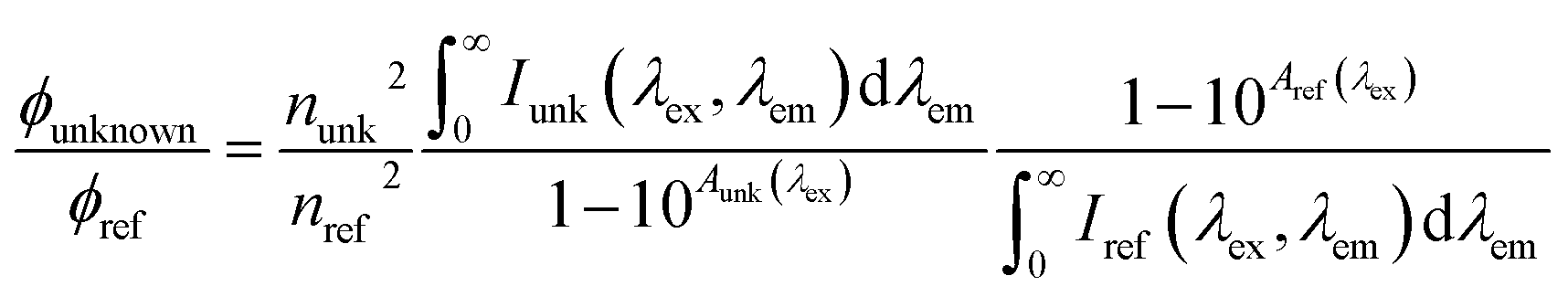
|
unk: unknown | Birks (1970)225 |
| ref: reference | Würth et al. (2013)226 | |||
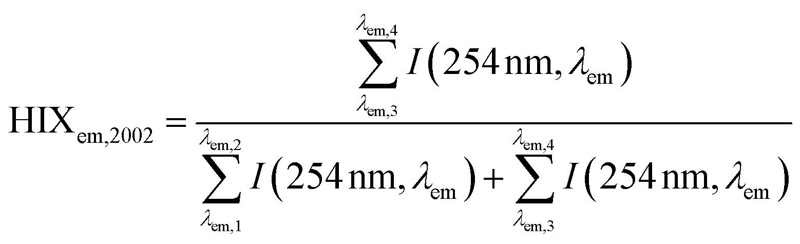
| Humification index | HIX |

|
λ em,1 = 300 nm | Zsolnay et al. (1999)227 Ohno (2002)228 |
| λ em,2 = 345 nm | ||||
| λ em,3 = 435 nm | ||||
| λ em,4 = 480 nm | ||||
|
||||
| Biological/freshness index | β/α |

|
Parlanti et al. (2000)229 | |
| Huguet et al. (2009)230 | ||||
| Wilson and Xenopoulos (2009)231 | ||||
| BIX |
|
|||
| Fluorescence index | FI |

|
McKnight et al. (2001)232 | |
| Cory and McKnight (2010)84 | ||||
| Maximum emission wavelength | λ em,max at λex = 310 nm | λ max(310) = max(I(310 nm, 310 − 590 nm)) | Parlanti et al. (2000)229 | |
| McKnight et al. (2001)232 | ||||
| λ em,max at λex = 370 nm | λ max(370) = max(I(370 nm, 370 − –710 nm)) | Wilson and Xenopoulos (2009)231 | ||
| Cory and McKnight (2010)84 | ||||
| Specific fluorescence intensity | SFI A |

|
Coble (1996)233 Alberts and Takács (2004)234 Jaffé et al. (2004)235 Hudson et al. (2007)236 Korak et al. (2014)75 | |
| SFI B |

|
|||
| SFI C |
|
|||
| SFI T |

|
|||
4.1 Apparent quantum yield
In practice, AQY compares the fluorescence of an unknown sample to a standard with a known quantum yield by calculating the ratio of the integrated fluorescence intensity (across all emission wavelengths) relative to the absorbance at the same excitation wavelength (Table 2). The same measurements are performed on a standard with a known quantum yield. Quinine sulfate in 0.1 N H2SO4 is well-characterized (Φf = 0.51)237 and a commonly used reference for humic substances.39,66,220,234,238 However, salicylic acid (Φf = 0.35) has been preferred for SEC studies over quinine sulfate in 0.1 N H2SO4 due to incompatibility of acidic solutions with the stationary phase of chromatography columns.66,239
The earliest studies reported ratios of fluorescence to absorbance (or color) rather than the formally defined AQY. For example, Kalle (1949) followed by Duursma (1965) and Christman and Ghassemi (1966) investigated linear relationships between fluorescence intensity and absorbance,164,240,241 the slope of which is related to AQY. Levesque (1972) and Hall and Lee (1974) fractionated samples with Sephadex and found the ratio of fluorescence to absorbance increased with decreasing molecular weight for a fulvic acid, extracts from leaves, sediment, and a lake sample.105,242 Zepp and Schlotzhauer (1981) formally calculated AQY for a range of aquatic and soil sources and noted that, despite breadth in origin, the range was remarkedly small (0.001–0.004), except for a sample from the Florida Everglades (0.012).67 AQY for most aquatic isolates is <0.02,39,66,220,238 with higher values (0.02–0.1) reported for specific contexts, such as marine and estuary environments,66,220,243 EfOM,38,244 pyrogenic organic carbon,245,246 and samples treated by physicochemical processes.247,248 In Alberts and Takács (2004),234 AQY was higher for fulvic acids than humic acids for 13 IHSS isolates. Overall, AQY values for DOM are small compared to pure, model organic compounds common in broader fluorescence inquiries such as tyrosine (Φf = 0.21),249 quinine sulfate (Φf = 0.51),237 and fluorescein (Φf = 0.79).250 However, model compounds leveraged as DOM building blocks, such as gallic-, syringic-, and vanillic acids, typically have quantum yields of similar magnitude to DOM.66
4.1.2.1 Molecular weight. For both aquatic samples and plant leachates, Stewart and Wetzel (1980)251 fractionated samples using Sephadex and dialysis, where the fluorescence-to-absorbance ratio (Fluor/Abs) increased with decreasing molecular weight following internally consistent trends within, but not across, samples (Fig. 7e). For example, the Fluor/Abs ratio for the <3.5 kDa fraction of leaf litter leachate was similar to the >3.5 kDa fraction from Lawrence Lake (Fig. 7e). Similarly, De Haan and De Boer (1987) fractionated lake samples using UF and presented a log-linear correlation between Fluor/Abs and molecular size (Fig. 7b).77 While this trend was strong, the concentration-weighted Fluor/Abs values from each fraction did not reconcile with the whole-water value, suggesting non-conservative mixing of optically active moieties.77 A note of caution, some early studies used different fluorescence excitation and absorbance wavelengths,77,116,251 whereas fundamental theory and current practice utilize the same wavelength.
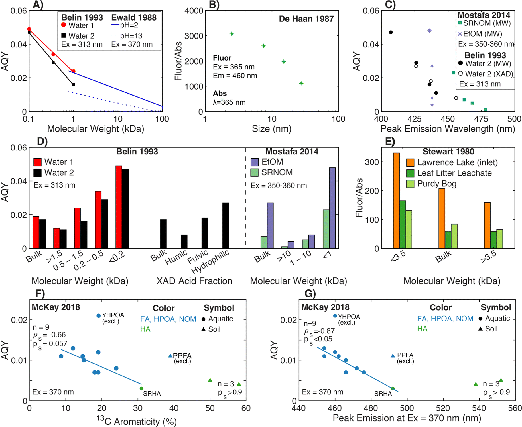 | ||
| Fig. 7 Relationship between fluorescence efficiency and either molecular weight, isolate fraction, peak emission wavelength, or different measures of aromatic carbon. Fluorescence efficiency is quantified through either fluorescence AQY (A, C, D, F, and G) or as the ratio of fluorescence-to-absorbance at discrete wavelengths (B and E). (A) AQY versus molecular weight for UF fractions252 plotted at the mid-point of each bounded molecular weight fraction. The unbounded fraction (>1.5 kDa) is not plotted. Regression lines are from Ewald et al. (1988).180 (B) Fluorescence-to-absorbance ratio (Fluor/Abs) versus molecular size for Lake Tjeukemeer DOM. Molecular size data are plotted at the midpoint for each bounded size fraction.77 (C) AQY versus peak emission wavelength for one water fractionated by both UF and XAD techniques252 and two endmembers fractionated by UF.38 (D) AQY versus either UF fraction or XAD fraction.38,252 (E) Fluor/Abs versus UF fraction.251 Fluorescence efficiency is reported using fluorescence at λex 360 nm and λem 460 nm relative to absorbance at 250 nm. AQY39versus (F) aromaticity (%) per sample calculated from 13C NMR data40–43 or (G) peak emission wavelength.39 Yukon HPOA (YHPOA) and Pahokee Peat Fulvic Acid (PPFA) isolates were excluded from the linear regression. | ||
Ewald et al. (1988) formally calculated the AQY for a fulvic acid that was isolated from a microbial culture inoculated with a soil actinomycete and fractionated by UF. For this narrow context, AQY decreased with increasing log-molecular weight following a pH-dependent, linear relationship (Fig. 7a).180 More representative of aquatic systems, Belin et al. (1993) fractionated two waters comparing UF and XAD techniques (Fig. 7a and d). For UF fractionation, AQY decreased as molecular weight increased following a sample-specific, log-linear relationship.252 Similar sample-specific trends of increasing AQY with decreasing molecular weight have been demonstrated for a broader range of DOM samples, including isolates (e.g., terrestrial and marine)70,186,253 and EfOM (Fig. 7d),38 but it has also been contradicted in deep oligotrophic waters.116
Although many studies have presented SEC chromatograms using absorbance and fluorescence detectors,118,254,255 Hanson et al. (2022)239 was the first to couple the responses from both detectors and calculate AQY as a function of elution volume. This coupling also required development of instrument correction factors for SEC. Within a single sample, Hanson et al. (2022) offers additional lines of evidence that AQY increases as molecular weight decreases for a surface water (Colorado, USA), two humic substance isolates, and ozonated samples. Comparing SEC chromatograms of AQY and DOC concentration, the DOM fraction with the highest AQY was associated with a relatively small fraction of the total organic carbon.239
4.1.2.2 Aromaticity. Compared to size fractionation, fewer studies have assessed AQY as a function of aromatic carbon content. As an indirect approach, XAD methods isolate fractions with more (HPOA) or less (transphilic acid, TPIA) aromatic carbon.139,256 In Belin et al. (1993), the humic acid isolate had lower AQY compared to the paired fulvic acid,252 which can be inferred as AQY decreasing with increasing abundance of aromatic carbon.1 Applying a conservative mass balance to fluorescence intensity for one lake sample, Belin et al. (1993)252 concluded that roughly 60% of the whole-water fluorescence intensity was attributed to the fulvic acid fraction, followed by hydrophilic acids (35%) then humic acids (5%). Baker et al. (2008)257 applied DAX-8 resin fractionation to 25 surface waters demonstrating that the Fluor/Abs ratio (Peak C to absorbance at 340 nm) was proportional to the fraction of whole-water DOC recovered in as hydrophilic DOM. There are mixed results about the impact of solid phase extraction on AQY. Although some studies show decreasing spectral slope after isolation with C18 cartridges,70,220 others report mixed outcomes for how solid phase extraction impacts fluorescence AQY.220,243,258
Although the aforementioned studies provide indirect evidence relating AQY and aromaticity, optical data from McKay et al. (2018)39 paired with 13C aromaticity data40–43 reveal two main trends (Fig. 7f). Across most aquatic isolates, AQY decreased with increasing aromaticity with a continuous, linear relationship across fulvic-dominated, aquatic isolates (NOM, HPOA, and FA) and SRHA. As a subset, humic acids (1 aquatic and 2 soil) showed no trend. Two fulvic-dominated isolates were outliers. Yukon HPOA (YHPOA), a winter baseflow HPOA isolate from the Yukon River,42 had a higher AQY than all other isolates. Similarly, Pahokee Peat fulvic acid (PPFA) from the Florida Everglades exhibited an AQY similar to aquatic isolates, despite this sample having a higher aromaticity based on 13C NMR.
Across diverse aquatic environments, there is an inverse relationship between AQY and peak emission wavelength. This trend could be predicted from first-principles relating the energy gap between S1 and S0 to non-radiative decay rates.52,225 In Ewald et al. (1988) and Belin et al. (1993), emission wavelengths of maximum fluorescence intensity shifted 30–50 nm between fractions, and maximum wavelengths increased as AQY decreased.180,252 In the latter study, there was good agreement between UF and XAD fractionation techniques for a single sample (Fig. 7c).252 This trend also held for UF-fractionated SRNOM but not EfOM, which showed no change in peak emission wavelength (Fig. 7c).38Fig. 7g shows that the trend generally held across the aquatic isolates in McKay et al. (2018).39 Similar to relationships with aromaticity (Fig. 7f), however, humic acids, YHPOA, and PPFA were exceptions.
Broadly, systematic relationships between AQY and molecular weight appear to hold for fractionated samples; however, variations in AQY should not be used to infer differences in molecular weight across samples. An inverse relationship between AQY and both aromaticity and peak emission wavelength holds across a range of isolates; however, future work is needed to investigate the outliers (e.g., YHPOA, PPFA, and EfOM). Lastly, the increased resolution gained by online measurements of AQY using SEC highlights a future opportunity for establishing relationships between AQY and DOM molecular size.
4.2 Specific fluorescence intensity (SFI)/relative fluorescence intensity
There are different approaches to calculate SFI with different unit conventions. For example, samples may be prepared at the same DOC concentration (e.g., 1, 10 or 100 mgC L−1) before measuring fluorescence,259,268–271 or samples may be analyzed as-is before dividing fluorescence intensities by the DOC concentration.235,261 The two approaches should yield equivalent information, assuming that (1) sample chemistry follows fundamental equations (Bouguer–Beer–Lambert law (eqn (1)) and linearized fluorescence (eqn (7))) and (2) best practices are followed for spectral corrections and instrument limitations (e.g., detector linearity). The units depend on the units of both fluorescence intensity (e.g., arbitrary units, counts per second, Raman units, or quinine sulfate equivalents) and DOC concentration (e.g., mgC L−1 or mmolC L−1), leading to units analogous to SUVA (e.g., RU L mgC−1, RU L gC−1 or QSU L mmolC−1).75,235,261,272 In some cases, captions or methods describe the normalization process, not the intensity units explicitly.273–275
There is an opportunity for the research community to be more explicit and consistent in unit conventions to facilitate inter-study comparisons and reduce ambiguity. It is important to note that diluting to a common DOC concentration does not negate the need for inner filter corrections as each sample has a unique absorbance spectrum. Care is needed when interpreting studies without spectral corrections.
SFI is the slope relating fluorescence intensity to DOC concentration.75 As early as 1968, Ghassemi and Christman compared different source waters using SFI.169 In addition to highlighting compositional differences, research has also leveraged contexts with little variability to predict DOC concentration from fluorescence.76,276 Across samples, stronger correlations between fluorescence intensity and DOC concentration indicate more homogeneity in DOM composition. In contexts with greater spatial and temporal variability, (e.g., diverse surface waters, variable land use, and changing hydrological conditions), relationships between DOC concentration and fluorescence exhibit site-specific slopes with lower correlation coefficients76,272,276 compared to narrower contexts.76,272,276 For example, consistent slopes are observed within narrow contexts, such as short-term sampling campaigns across an estuary salinity gradient dominated by conservative dilution.71,263 Therefore, using fluorescence as a proxy for DOC concentration depends on an underlying assumption of constant SFI.
4.2.2.1 Aromaticity. SFI was not introduced as a quantitative surrogate for a specific compositional characteristic, but differences were often interpreted through the lens of aromatic carbon. Using soil isolates prepared at comparable concentrations, Mukherjee and colleagues (1964, 1971)270,277 attributed fluorescence to aromatic moieties with electron donating groups or conjugated, unsaturated compounds with resonance. Datta et al. (1971)270 reported higher SFI for fulvic acids than humic acids and attributed differences to aromaticity. Later, Senesi, Miano, and colleagues measured excitation, emission, and synchronous scans for soil and aquatic isolates prepared at a constant concentration. These studies proposed SFI as a tool to distinguish humic acids from fulvic acids, noting that fulvic acids consistently exhibited higher SFI and blue-shifted emission maxima.268,275,278,279 Focused on soils, Senesi et al. (1991)268 attributed these differences to fulvic acids having less aromatic condensation, less conjugation between chromophores, and higher abundance of electron-donating groups. Although independent measures were not presented, the study advocated for complementary techniques like NMR in future work.
There are some contradictions in literature relating SFI and aromaticity between intra- and inter-sample comparisons. Croue et al. (2000) fractionated SRNOM with XAD resin, comparing SFI at excitation 320 nm between 9 fractions. In general, SFI increased as relative hydrophilicity of the fraction increased. For example, the hydrophilic base fraction accounted for 0.04% of the total carbon but was about four times more fluorescent.125 This study would suggest that SFI increases as aromaticity decreases. However, in McKnight et al. (2001),232 SFI was calculated at excitation 370 nm with paired 13C aromaticity measurements (n = 6), and the median SFI was higher for terrestrial endmembers with higher aromaticity than microbial endmembers (Fig. 8a). Since the highest SFI in the whole dataset (n = 11) was a microbial endmember, fluorescence index (FI) was justified as a better measure to differentiate sources.232 Alberts and Takács (2004)234 paired fluorescence measurements with IHSS-reported 13C NMR40,41 and carboxyl and phenol content280 for 13 IHSS isolates. SFI near Peak C (λex 330 nm, λem 440 nm) did not correlate with the relative abundance of functional groups determined by NMR. Using titration, however, SFI correlated positively with carboxyl content and inversely with phenolic content for the fulvic acids. The same correlations were not significant for humic acids, where SFI only correlated with SUVA254.234
 | ||
| Fig. 8 Relationship between specific fluorescence intensity (SFI) and either molecular weight or different measures of aromatic carbon. (A) SFI versus aromaticity (%) per sample calculated from 13C NMR data for fulvic acids.232 (B) SFI versus aromaticity (%) per sample calculated from 13C NMR data pairing optical39 and NMR data.40–43 (C) Estimated (Est.) SFI (calculated from PARAFAC components, see ESI Text 4†) versus the relative abundance of condensed aromatic and polyphenolic formulae (%) per sample calculated based on AImod132 from FT-ICR MS data.35 (D) SFI of UF molecular weight fractions from lakes, soils, and leaf leachates.100 (E) Whole-water (<0.2 μm) SFI versus the relative abundance of whole-water DOC (%) in two UF fractions.100 (F) FI versus UF molecular weight fractions.38,44 | ||
The optical data in McKay et al. (2018) illustrates a discontinuity between humic- and fulvic acid isolates. Fig. 8b shows two distinct groups in the data. Isolates from aquatic fulvic acids, HPOA and NOM formed one group where Peak C SFI (λex 320 nm, λem 440 nm) and 13C aromaticity correlated (ρS = 0.93, n = 9). Humic acids formed a second group where Peak C SFI was relatively insensitive to 13C aromaticity. Detailed in ESI Text 4,† Peak C SFI was estimated by reconstructing intensities from PARAFAC data presented in Kellerman et al. (2018),35 because peak intensities were not reported. Fig. 8c suggests that Peak C SFI increases as relative abundance increases only at low abundances of aromatic and polyphenolic formulae. When abundance exceeds about 25%, the estimated SFI is comparatively insensitive to compositional changes measured by FT-ICR MS.
4.2.2.2 Molecular weight. Using Sephadex separation, Ghassemi and Christman (1968) characterized a river sample (British Columbia, Canada) by GPC and reported chromatograms of DOC concentration, absorbance (350 nm), and fluorescence intensity (λex 360 nm, λem 415 nm). The elution volume at which the maximum signal occurred was lower for both DOC concentration and absorbance compared to fluorescence, suggesting SFI increased in smaller molecular weight fractions.169 At similar fluorescence wavelengths, several other studies have reported higher SFI associated with smaller molecular weight for lakes105 and extracts from soil, leaves, and sediment.105,281
Using UF, Buffle et al. (1978)100 fractionated eight natural waters, five soil extracts, and four leaf extracts into three molecular weight fractions (0.2 μm–10 kDa, 0.21–10 kDa, and <0.21 kDa). Compared to the filtered whole-waters (<0.2 μm), median SFI values were higher in the smaller weight fractions (Fig. 8d). Applying a mass balance to DOC concentration, Fig. 8e shows that the whole-water SFI increased as (1) the fraction of whole-water DOC recovered in the middle fraction (0.21–10 kDa) increased (ρS = 0.87, n = 15) and (2) the DOC recovered in the large fraction (0.2 μm–10 kDa) decreased (ρS = 0.87, n = 15). There was no statistically significant correlation between SFI and the fraction of whole-water DOC recovered in the small fraction (<0.2 kDa) (ps = 0.2).
Multiple studies have presented additional evidence supporting greater SFI in smaller molecular weight fractions, but a pattern of inconsistencies with the smallest weight fractions are noted.77,282,283 For example, in De Haan and De Boer (1987), SFI (λex 365 nm, λem 470 nm) was highest in the intermediate fractions (5–35 nm) and smaller in both remaining (<5 nm and >35 nm) fractions.77 For a membrane bioreactor, Xiao et al. (2018)284 noted a discontinuity for the <0.5 kDa fraction with lower than expected SFI and relatively little change in SFI at molecular weights >10 kDa. For a sediment sample, Hayase and Tsubota (1985) fractionated humic- and fulvic acid isolates into five molecular weight fractions ranging from <10 kDa to >300 kDa, and SFI increased with decreasing molecular weight. Interestingly, SUVA at the excitation wavelengths of maximum fluorescence intensity (320 and 480 nm for fulvic- and humic acid isolates, respectively) had opposite correlations with SFI. For humic acids, SUVA480 correlated positively with SFI, but SUVA320 correlated negatively with SFI for fulvic acids. This difference was attributed to SUVA480 increasing with decreasing humic acid molecular weight fraction,218 which contradicts the trend most often observed (Section 3.1.2). In Fig. 8f, two IHSS isolates followed the trend of increasing SFI as molecular weight fraction decreased. The wastewater endmember (EfOM) deviated with similar a SFI in the largest and smallest fractions and an uncharacteristically high SFI in the bulk water, warranting further investigation.
Between 1999 and 2004, several studies by Alberts, Takács, and colleagues used UF and/or SEC to characterize DOM in aquatic environments using SFI near Peak C.186,187,285,286 Some samples, such as Suwannee River and estuarine UF fractions, matched expectations showing increasing SFI with decreasing molecular weight.187,285,286 However, some waters had higher SFI in the middle fraction (10–50 kDa) compared to the small fraction (<10 kDa), and differences between the Peak A and C regions.187 Although some studies do not appear to correct for inner filter effects, the lower SFI in the small fraction cannot be explained by inner filtering. If absorption coefficients typically increase with molecular weight (Section 3.1), then SFI would be suppressed more in larger fractions. More likely, inconsistencies can be attributed to the differences in membrane cut-off relative to the expected weight distribution in DOM. A 10 kDa membrane cut-off may offer appropriate resolution to fractionate soil isolates, but most carbon by mass is associated with <10 kDa fractions in aquatic systems.1,100 By using SEC to fractionate two samples, the increased resolution in Alberts et al. (2002) supports increasing SFI with decreasing molecular weight for wavelengths near Peaks A and C.187
Molecular weight resolution is further improved with online fluorescence and DOC concentration detectors for SEC analysis. Her et al. (2003, 2004)262,269 characterized contrasting samples, including groundwater, hypereutrophic surface water, secondary wastewater effluent, and algal organic matter. SUVA254 decreased with decreasing molecular weight, but SFI near Peak C (λex 337 nm, λem 423 nm) either remained relatively constant or increased. In samples from microbiologically active systems, the large molecular weight peak, commonly associated with biopolymers,117 exhibited higher SFI near Peak T (λex 278 nm, λem 353 nm) compared to Peak C.118,269 Allpike et al. (2005) presented additional evidence that SFI near Peak T increased as both SUVA254 and molecular weight decreased.254
Overall, there appears to be inconsistency in the logic relating the SFI near Peak C to aromaticity and molecular weight. Within aquatic systems, Fig. 8b and c shows increasing SFI with increasing aromatic carbon for a breadth of aquatic isolates. However, multiple lines of evidence support increasing SFI with decreasing molecular weight (Fig. 8d–f). Yet, the conventional interpretation is that more aromatic DOM is associated with larger molecular weights. This inconsistency could be explained by the increases in AQY as molecular weight decreases (e.g., lower molecular weight DOM is less prone to deactivation of singlet excited states through intramolecular energy transfer).49,52,53 Even though fewer photons are absorbed per unit carbon (i.e., lower SUVA), the AQY increases to yield a higher SFI.
4.3 Humification index (HIX)


In the same year (1999), both Kalbitz et al.260 and Zsolnay et al.227 proposed independent definitions of HIX. Kalbitz et al. (1999) calculated peak ratios from synchronous fluorescence scans (Δλ = 18 nm) proposing 3 different definitions (HIXsyn,400/360, HIXsyn,470/360, and HIXsyn,470/400). Synchronous scans are a two-dimensional spectrum that steps through a range of values for λex and λem, while maintaining a constant offset (Δλ = λem − λex), effectively measuring a diagonal cross-section of a three-dimensional EEM. HIXsyn,400/360 and HIXsyn,470/360 had a high correlation coefficient (r) between each other (r = 0.91), and comparisons with other characterization techniques used HIXsyn,470/360.260 In a subsequent paper, the list expanded defining a new ratio at lower wavelengths for whole-waters (HIXsyn,390/355) compared to fulvic acids (HIXsyn,470/360); HIX values between whole-waters and paired isolates were strongly correlated (ρ > 0.88).259 In contrast, Zsolnay et al. (1999) defined HIXem,1999 by integrating and then dividing areas under two regions of an emission scan (Table 3).227 The emission scan approach has since gained in popularity, in part due to the ease of collecting EEMs and availability of fluorometers with charge-coupled device detectors. Kalbitz et al. (2003) noted that HIXem,1999 yielded stronger correlations with other physicochemical properties than the synchronous scan approaches.287 Another definition (HIXem,2002) was proposed by Ohno (2002) using the sum of both integrated areas in the denominator to mitigate inflating uncertainty when blue-shifted (i.e., lower emission wavelength) intensities are low.228 In a published comment, Zsolnay (2002) concurred that the revised approach has statistical advantages but also argued that it may compress the scale and decrease the sensitivity to differentiate samples with high HIX values.288
Both definitions are related to one another following eqn (11) with the derivation in ESI Text 3.† Regardless of the definition, the intent of the surrogate is similar; however, a meta-analysis of >700 samples showed that neither definition was strongly correlated with peak emission wavelength.45
 | (11) |
A challenge with some early studies is the lack of specificity regarding inner filter corrections. Some spectra were measured at constant DOC concentration but did not explicitly state if spectra were corrected for inner filter effects.259,260 To minimize bias, Zsolnay et al. (1999)227 diluted samples and applied primary inner filter corrections, but the correction approach is inconsistent with common practice today.59,79 Independent of fluorescence characteristics, a sample with a higher spectral slope (or E2:E3) would introduce bias that increases HIX values. Systematic bias is introduced, because blue-shifted fluorescence would be suppressed due to secondary inner filtering. Since DOM absorbance spectra typically follow exponential decay, eqn (8) shows that the correction factor increases as wavelength decreases. If studies did not correct for inner filter effects, the reported correlations between HIX and chemical characteristics are biased to some extent, and it may not be possible to attribute relationships uniquely to fluorescence characteristics.
In the Kalbitz et al. (1999 and 2000) papers, the primary objective evaluated HIXsyn as a surrogate to either (1) characterize soil organic matter extracts or (2) understand the impact of land use on whole-water optical characteristics in hydraulically connected systems. Using fulvic acid isolates from water extracted soil, groundwater, and surface water, HIXsyn,470/360 positively correlated with SUVA285 (r = 0.85) and inversely correlated with the carbon-to-nitrogen ratio (C/N) (r = −0.63).260 The relative abundance of aromatic carbon (C![[double bond, length as m-dash]](https://www.rsc.org/images/entities/char_e001.gif) C stretch at 1620 cm−1) and carboxyl groups (CO stretch at 1725 cm−1) was estimated using FTIR.260 HIXsyn,470/360 was positively correlated to the relative intensity of aromatic carbon (r = 0.71) and inversely correlated to the ratio of aromatic to carboxyl intensities (1725 cm−1/1620 cm−1, r = −0.69).260 These results supported HIXsyn,470/360 as a surrogate for aromaticity based on either direct (FTIR) or indirect (SUVA285) measurements.260 In Kalbitz et al. (2000),259 HIXsyn for paired whole-water and fulvic acid isolates were more strongly correlated (r = 0.89) than SUVA285 (r = 0.62). Additionally, HIXsyn,390/355 values for whole-waters positively correlated with aromatic carbon by FTIR (r = 0.66) and inversely correlated with the C/N ratio (r = −0.48).259 Collectively, chemical composition correlated more strongly with HIXsyn than SUVA285, rationalizing an advantage of fluorescence to infer differences in aromaticity without isolating fulvic acids.259 One disadvantage of these studies is that FTIR is a semi-quantitative assessment of aromaticity, whereas SUVA has strong support from 13C NMR measurements.2
C stretch at 1620 cm−1) and carboxyl groups (CO stretch at 1725 cm−1) was estimated using FTIR.260 HIXsyn,470/360 was positively correlated to the relative intensity of aromatic carbon (r = 0.71) and inversely correlated to the ratio of aromatic to carboxyl intensities (1725 cm−1/1620 cm−1, r = −0.69).260 These results supported HIXsyn,470/360 as a surrogate for aromaticity based on either direct (FTIR) or indirect (SUVA285) measurements.260 In Kalbitz et al. (2000),259 HIXsyn for paired whole-water and fulvic acid isolates were more strongly correlated (r = 0.89) than SUVA285 (r = 0.62). Additionally, HIXsyn,390/355 values for whole-waters positively correlated with aromatic carbon by FTIR (r = 0.66) and inversely correlated with the C/N ratio (r = −0.48).259 Collectively, chemical composition correlated more strongly with HIXsyn than SUVA285, rationalizing an advantage of fluorescence to infer differences in aromaticity without isolating fulvic acids.259 One disadvantage of these studies is that FTIR is a semi-quantitative assessment of aromaticity, whereas SUVA has strong support from 13C NMR measurements.2
Defining the emission spectra approach, Zsolnay et al. (1999)227 assessed how fluorescence could differentiate DOM leached for different soil treatments. Fumigation with chloroform released DOM with blue-shifted fluorescence and a lower SFI relative to dried soil. The interpretation linking increased HIXem,1999 to more condensed, polyaromatic carbon was made by inference from previous studies,123,180,252,289,290 not direct evidence. Two of the previous studies,180,252 also described in Section 4.1, reported shifts in peak emission wavelength for both UF and XAD fractionation. Importantly, Belin et al. (1993) cites previous work256,291 for how aromaticity (primary) and molecular weight (secondary) are confounding factors in XAD fractionation. Also referenced, Kumke et al. (1995) reported a positive correlation between the wavelength of maximum fluorescence intensity and aromaticity for polycyclic aromatic hydrocarbons (PAHs), not humic substances.289 Overall, the definition of HIXem,1999 was not originally paired with a secondary, quantitative measure for aromaticity.
With soil microcosm experiments, Kalbitz et al. (2003) used 1H NMR to demonstrate that HIXem,1999 positively correlated with percent aromatic protons and negatively correlated with the proportion of oxygen-containing functional groups (Fig. 9a and b).287 NMR data correlated more strongly with HIXem,1999 than HIXsyn,460/345, strengthening the utility of the emission-based approach.287
 | ||
| Fig. 9 Relationship between humification index (HIX) and either molecular weight or different measures of aromatic carbon. HIXem,1999versus (A) aromatic proton abundance and (B) oxygen-containing group abundance.287 (C) HIXem,1999versus the relative abundance of condensed aromatic and polyphenolic formulae (%) per sample calculated by AImod132 from FT-ICR MS data.35 (D) HIXem,1999versus % aromaticity per sample calculated from 13C NMR pairing optical39 and NMR data.40–43 (E) HIXem,1999versus molecular weight determined by SEC and UV detection at 254 nm.292–296 Legend indicates calculation method (Mwvs. Mn) when available. (F) HIXem,2002versus % aromaticity per sample pairing optical39 and 13C NMR data.40–43 (G) HIXem,1999versus UF fraction including a boxplot with all data and bar chart with two samples.297 (H) HIXem,2002vs. weight-averaged elution time from SEC for samples fractionated by UF for a DOM isolate (SRNOM) and wastewater effluent (EfOM).38 HIX values were not reported in the initial study but calculated from corrected EEMs. Applying a quality control approach,45 HIXem,2002 is not reported for SRNOM in the >10 kDa fraction due to spectral noise. For EfOM, the >10 kDa sample was excluded from the regression. | ||
4.3.2.1 Aromaticity. Since this initial cohort of studies, data from Kellerman et al. (2018)35 presents the strongest evidence for HIXem,1999 as a surrogate for aromatic carbon. Fig. 9c shows that HIXem,1999 increased linearly with the relative abundance of condensed aromatic and polyphenol formulae. The positive intercept implies a positive HIXem,1999 value is possible with no contributions from these aromatic formulae. However, electrospray ionization does not ionize all aromatic moieties in DOM,143 and excitation without aromatic moieties is unlikely.
Fig. 9d and f compares HIX calculation methods using data from McKay et al. (2018).39 For HPOA and fulvic acid isolates from aquatic systems, there is a positive correlation between HIX and aromaticity by 13C NMR for both HIX calculation methods. Extrapolating HIXem,1999 tracks towards PPFA, the only soil-derived fulvic acid in the dataset, which is not the case for HIXem,2002. Similar to AQY (Fig. 7f), HIXem,2002 is relatively insensitive to 13C aromaticity for humic acids. Fig. 9f illustrates the sensitivity loss for HIXem,2002 to differentiate isolates as described by Zsolnay (2002).288 With the exception of marine isolates and the Antarctic endmember, HIXem,2002 for all other isolates was between 0.92 and 0.98 and relatively insensitive to changes in 13C aromaticity.
Several other papers demonstrate quantitative relationships between HIX and measures of aromatic carbon for narrower contexts. For example, Zhou et al. (2021) incubated 4 diverse DOM sources (i.e., algal-, macrophyte-, sewage-, and soil-derived). Not only did HIXem,1999 increase, but principal component analysis (PCA) identified strong associations between HIXem,1999 and two FT-ICR MS measures of aromatic carbon (i.e., polyphenolic abundance and AImod).298 Using a HIXsyn approach, Hur et al. (2021) extracted humic acids from soils and sediments and showed that HIXsyn correlated positively with aromatic carbon and negatively with o-alkyl carbon.299 In Kellerman et al. (2015) for Nordic lakes, HIXem,2002 was strongly associated with aromatic, oxygen-rich compounds measured by FT-ICR MS.300 Finally, Wagner et al. (2015) reported an association between HIXem,2002 and less condensed aromatic structures, such as polyphenols, in the Florida Everglades.183
4.3.2.2 Molecular weight. Most studies have focused on demonstrating within-sample relationships using UF for narrow sample contexts. Huguet et al. (2010)297 presented one of the largest datasets of UF fractionated samples with a narrow geographic context of the Seine and Gironde estuaries (France). Aggregating the entire data set, HIXem,1999 generally increased as molecular weight increased (Fig. 9g). However, there is substantial overlap between fractions, where molecular weight could not be uniquely inferred from HIXem,1999 alone. Contrasting endmembers in Fig. 9h, HIXem,2002 was inversely correlated with weight-averaged elution time from SEC (UV254 detector) for <10 kDa fractions.38 However, the largest fraction (>10 kDa) of EfOM was an outlier. A similar disconnect was reported for leaf litter extracts, where HIXem,1999 decreased as molecular weight increased from 10 to 100 kDa.301
In other SEC studies using UV detection, Fig. 9e shows mixed trends. Quantitative comparisons between studies are challenging due to different SEC methods, calibration standards, and reporting conventions (Mwvs. Mn). Hur (2011) offers the most diverse dataset including EfOM, algal DOM, terrestrial DOM, and plant-derived DOM; HIXem,1999 increased as Mn increased.296 Similar positive correlations were reported for stormwater runoff,292 sediments from two locations,302 and a single source water subjected to UF fractionation and coagulation.293 However, HIXem,1999 was insensitive to molecular weight across different wastewaters295 and leachates from plant biomass and manure residues.294 Across a water treatment process (e.g., nanofiltration, granular activated carbon) in Köhler et al. (2016),303 HIXem,2002 was positively correlated with the average molecular weight of the humic substance fraction, according to the Huber et al. (2011)117 SEC method. Lee et al. (2019) coupled a fluorescence detector with SEC to calculate HIXem,1999 from emission spectra taken at one minute intervals. Testing four IHSS isolates, elution profiles supported increasing HIXem,1999 with increasing apparent molecular weight.304
As a whole, these studies reveal opportunities for further inquiry and convergence in the DOM community. Relationships between HIX and either aromaticity or molecular weight appear to have contextual limitations. Correlations for fulvic-acid dominated isolates (NOM, HPOA, or FA) may not be broadly applicable to whole-waters, EfOM, or humic acid isolates, of which the latter two both showed lower sensitivity to aromaticity. Within-sample trends appear to be stronger than comparisons between samples of different origins, urging caution against using differences in HIX to infer differences in molecular weight between sources. Between XAD fractionation (where non-humic substances are not recovered) and the reliance on UV detection for SEC (which does not detect non-chromophoric DOM), the aromaticity- and SEC-derived relationships in Fig. 9 are limited. SEC studies that combine DOC concentration and UV absorbance detection can help resolve the molecular weight fractions of DOM that are non-chromophoric.
4.4 Biological index, Freshness Index, or β/α
Huguet et al. (2009)230 introduced the acronym BIX but interestingly did not define it as Biological Index, as commonly referred to today. The acronym was introduced as the “index of recent autochthonous contribution”. The earliest known paper that attributed the name Biological Index to BIX was Carstea et al. (2009).305 Reducing ambiguity, Huguet et al. (2009)230 explicitly defined a calculation method for BIX (Table 2) as the ratio of two fluorescence intensities (380 to 430 nm) measured at 310 nm excitation. Huguet et al. (2009) also defined an interpretation scale, where BIX values between 0.6–0.7 have low autochthonous contributions and BIX value >1 have high contributions. That paper concluded that HIX and BIX are complementary indices and could capture different characteristics of DOM composition. Across an estuarine-marine gradient, HIX responded to changes in the DOM fluorescence at lower salinity (S < 25), where BIX was comparatively insensitive, yet both surrogates trended in opposite directions at higher salinity.
Wilson and Xenopoulos (2009)231 applied the same concept using a different calculation method. Continuing to use the term β/α coined by Parlanti et al. (2000), Wilson and Xenopoulos (2009) modified the denominator to calculate the maximum fluorescence intensity between λem 420–435 nm (Table 2). They showed that β/α increased as both the percentage of continuous cropland and total dissolved nitrogen increased.231 A meta-analysis by Korak and McKay (2024)45 compared the fixed and variable λem calculation methods across >700 samples and showed good agreement at low BIX values with small, systematic deviations at higher values.
Of these three early papers, none of them used the term “Freshness Index”, which is also commonly used today. To the best of our knowledge, the earliest reference for this term is the highly cited review article by Fellman et al. (2010).267
4.4.2.1 Molecular weight. Of the three genesis papers,229–231 none paired the optical data with independent measures of aromaticity or molecular weight. Huguet et al. (2010)297 was the first to fractionate samples with UF. For the two estuarine gradients (i.e., Seine and Gironde rivers), sample-specific trends generally held where BIX increased as molecular weight decreased (Fig. 10a). Aggregating the entire dataset, boxplots show that differences in BIX were most pronounced in the smallest molecular weight fractions (i.e., <0.5 kDa and 0.5–1 kDa) with no difference between the 1–3 and >3 kDa fractions (Fig. 10a). Since previous work1,297 has shown more than 50% of DsOM in freshwaters, quantified as DOC concentration, is typically associated with a >1 kDa fraction, we caution using BIX to infer differences in molecular weight between whole-water samples. Since the Huguet et al. (2010)297 study, there is a noticeable gap in the literature pairing BIX with independent characterization techniques, recognizing an opportunity for future work to prioritize diverse DOM sources.
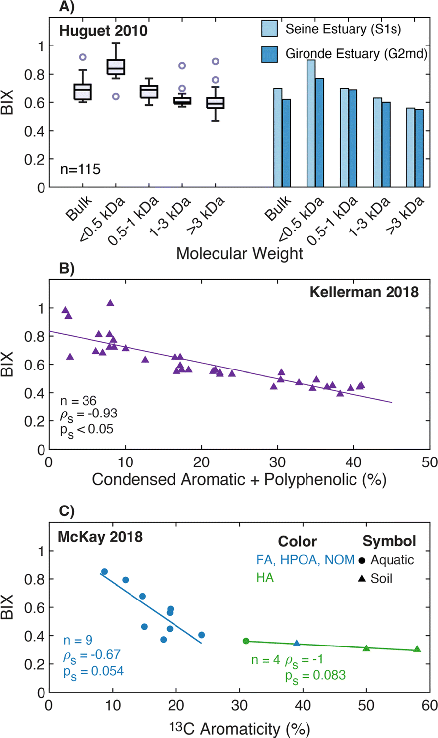 | ||
| Fig. 10 Relationship between biological index (BIX) and either molecular weight or different measures of aromatic carbon. (A) BIX versus UF fraction including a boxplot with all data and bar chart with two samples.297 (B) BIX versus the relative abundance of condensed aromatic and polyphenolic formulae (%) per sample calculated by AImod132 from FT-ICR MS data.35 (C) BIX versus % aromaticity per sample calculated from 13C NMR.39–43 | ||
Following one source water across an engineering treatment gradient, Köhler et al. (2016) presented an inverse, linear relationship between BIX and the relative abundance of the humic substance fraction,117 as determined by SEC with DOC concentration detection. A multilinear regression was presented to predict the concentration of low molecular weight neutral compounds using HIXem,2002 and β/α as predictors.303
4.4.2.2 Aromaticity. Like HIX, data from Kellerman et al. (2018)35 presents the strongest evidence across a large gradient of environmental systems of an inverse relationship between BIX and relative abundance of condensed aromatic and polyphenolic formulae (Fig. 10b). A similar inverse correlation between BIX and 13C aromaticity was observed for aquatic isolates (Fig. 10c).39 In contrast to Fig. 7F for AQY, neither YHPOA nor PPFA were outliers compared to the other isolates (Fig. 10c). YHPOA followed the same inverse correlation as other aquatic isolates. Unlike HIXem,1999, the soil-derived fulvic acid (PPFA) followed a similar trend as the humic acids. Notably, the slope was shallower for humic acids compared to aquatic, fulvic acid-dominated isolates. The disconnect between sample groups in Fig. 10c urges caution between generalizing interpretations across contexts.
Although these analyses provide strong evidence for BIX as a surrogate for aromatic carbon, the context is dominated by isolates (Fig. 10b and c), with NOM isolates obtained using reverse osmosis underrepresented compared to XAD isolates.35,39 Since BIX was originally defined as a surrogate for microbial exudates, differences in DOM recovery by XAD resins may hinder generalizations to whole-waters due to material not recovered during XAD isolation. For example, fulvic acids have been attributed to <20% of whole-water DOM (measured as DOC) in autochthonous Antarctic lakes compared to 30–60% of DOM more broadly across freshwaters.1,2,306 As a result, aromaticity generalizations to whole-waters may not be well-supported unless strong agreement is observed between paired BIX measurements of whole-waters and isolates.
4.5 Fluorescence index (FI)
 | (12) |
 | (13) |
The first objective in McKnight et al. (2001) was to leverage differences in the chemical composition of fulvic acids (e.g., aromaticity) to differentiate sources using a fluorescence surrogate. Previous work showed that aromaticity was higher for terrestrial (25–30%) compared to microbial (12–17%) fulvic acids,306,307 which would change fluorescence spectra.308 The second objective assessed if FI of the whole-water was a good surrogate for the isolated fulvic acid. Spanning samples collected from the from the contiguous U.S. to the dry valleys of Antarctica, isolates from microbial endmembers (without higher plant inputs) had higher FI values (1.7–2.0) compared to terrestrial endmembers (1.3–1.4) with higher plant inputs.232
McKnight et al. (2001) presented direct evidence of an inverse relationship between FI and 13C aromaticity for aquatic fulvic acids (Fig. 11a). Although there is a strong relationship, the study urged caution using FI as a generalized, quantitative surrogate for two reasons. First, extrapolating the regression models would yield an unrealistic, negative aromaticity at FI values >2.1, which were also observed in whole-water samples from Antarctic lakes232 (Fig. 11b) and more recently in wastewater effluents.38,295 Second, although the correlation was strong for fulvic acids, generalizing to whole-waters would require verifying that the regression holds with the non-humic fraction included.
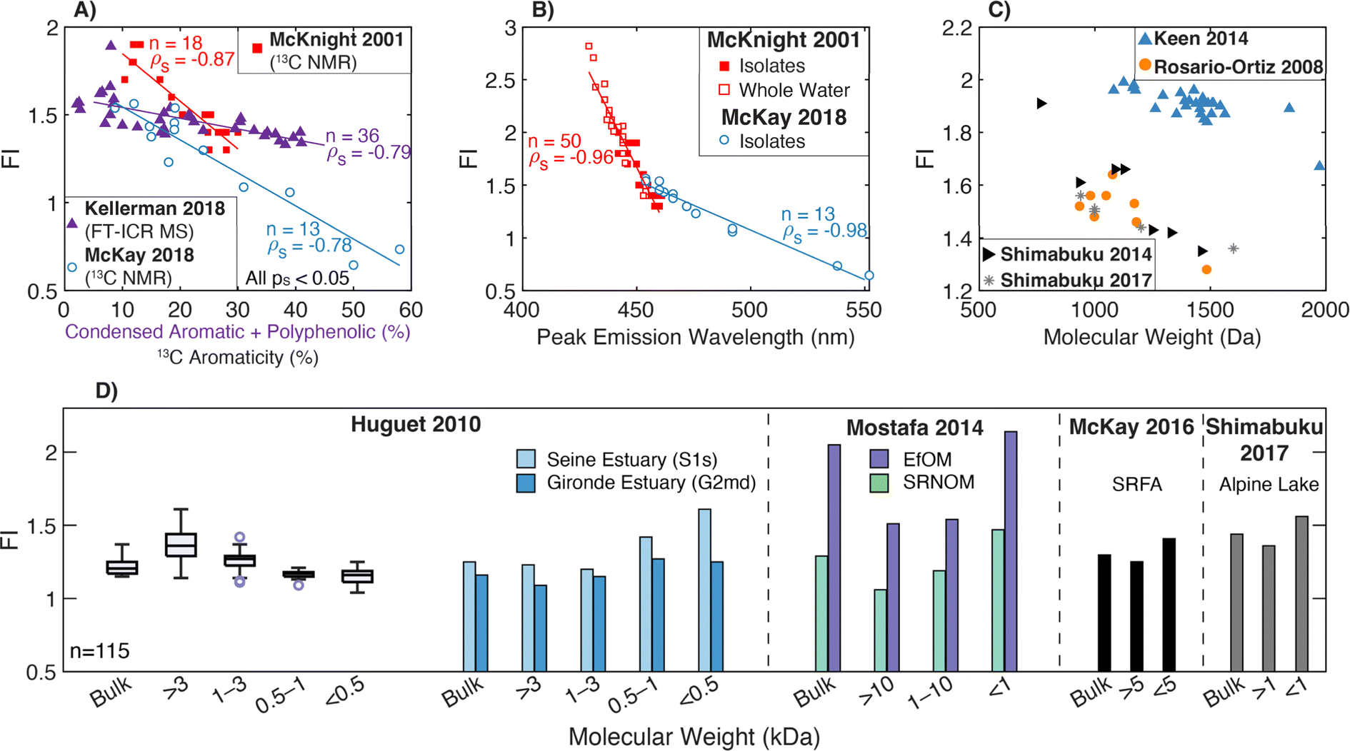 | ||
| Fig. 11 Relationship between fluorescence index (FI) and either molecular weight, peak emission wavelength, or different measures of aromatic carbon. (A) FI versus % aromaticity per sample calculated from 13C NMR39–43,232 or the relative abundance of condensed aromatic and polyphenolic formulae (%) per sample calculated by AImod132 from FT-ICR MS data.35 (B) FI versus the peak emission wavelength at excitation wavelength of 370 nm.39,232 (C) FI versus weight-averaged molecular weight (Mw) by SEC with a UV254 detector.293,295,309,323 (D) FI versus nominal molecular weight fraction following UF fractionation.38,44,293,297 | ||
Both studies84,232 advocated for reporting FI with the peak emission wavelength to confirm that FI increased as peak emission wavelength decreased. Although not originally plotted, Fig. 11b shows a strong inverse correlation between FI and peak emission wavelength with continuity across the fulvic acids and whole-waters in the 2001 paper.232 Lastly, a post-hoc analysis of the 2001 data supports a positive correlation between peak emission wavelength and 13C aromaticity for aquatic fulvic acids (r = 0.86, n = 18). Croue et al. (2000)125 concentrated (RO and nanofiltration) and fractionated (XAD) four surface waters, also reporting a positive correlation between 13C aromaticity and peak emission wavelength at excitation 320 nm (R2 = 0.61, n = 25).
4.5.2.1 Aromaticity. Using the relative abundance of condensed aromatic and polyphenolic formulae measured by FT-ICR MS, Kellerman et al. (2018)35 also shows that relative abundance decreased as FI increased (Fig. 11a). However, scatter in the data increased for relative abundances <20%. Optical data from McKay et al. (2018) shows a similar trend (Fig. 11a). Unlike AQY, HIX, or BIX, Fig. 11a and b for McKay et al. (2018) show an internally consistent correlation spanning the entire dataset from aquatic fulvic acids through soil humic acids. Although each of these studies show internally consistent correlations, generalizing to whole-waters requires caution due the limited context of XAD isolation, which does not recover the non-humic fraction known to contribute to whole-water fluorescence.238
4.5.2.2 Molecular weight. In the genesis studies,84,232 FI was not proposed as a surrogate for molecular weight. However, studies have recognized that DOM aromaticity and molecular weight often correlate.253,256,291 For example, Fig. 11d shows internal consistency within single samples fractionated by UF, where FI increased as molecular weight decreased for riverine and estuarine samples,297 an alpine lake,293,309 SRNOM,38 and wastewater effluent.38 Other papers showed similar consistency.253,310–312 Despite internal consistency for single samples, Fig. 11d illustrates that within a nominal size fraction, a wide range of FI values should be expected between source materials, and inverse interpretations of molecular weight between waters should not be made using FI. For example, the 1–10 kDa fraction of wastewater effluent had the same FI as the <1 kDa fraction from SRNOM. Fig. 11c contrasts two studies that used the same SEC instrument (UV detection) but different calibration standards.295,309 In Shimabuku et al. (2014), there was an internally consistent gradient across a fractionated sample that also aligned with other surface waters.309 However, wastewater samples from 8 facilities in Keen et al. (2014) had a comparatively smaller change in FI relative to the range of Mw values.295 Romera-Castillo et al. (2014) used preparative SEC to fractionate 4 samples from the Florida Everglades into 7 fractions. FI increased with decreasing size except for the smallest fraction where signals were near baseline.313
Interestingly, two studies by Shimabuku and colleagues293,309 showed that FI may contradict other lines of evidence regarding aromaticity and molecular weight. Using granular activated carbon (GAC) column tests, effluent at the beginning of the run (low bed volumes) had both lower SUVA254 and FI, which contradicts expectations of an inverse correlation between surrogates.293 In addition, SEC characterization of influent and effluent samples found that Mw was inversely related to FI (R2 = 0.91) but not SUVA254. Connecting optical surrogates to the role of molecular sieving in GAC separation, the study postulated that FI may be more dependent on molecular weight than aromaticity. Another study309 drew similar conclusions using coagulation and powdered activated carbon after observing greater competition between DOM and micropollutants in source waters with high FI. These studies corroborated results from Schreiber et al. (2005) that also defied conventional interpretations, where GAC preferentially removed small molecular weight chromophores but spectral slope increased.314 As a whole, the interplay of chemical sorption versus physical sieving by GAC may offer a unique opportunity to question causation versus correlation for optical surrogates and their dependence on aromaticity and molecular weight.
5 Conclusions and future opportunities
This critical review traced the genesis and assessed the continued inquiry of absorbance and fluorescence spectroscopy as surrogates for DOM aromaticity and molecular weight. Our analysis raises several findings that warrant further study.First, more caution is needed when interpreting specific optical surrogates as unique indicators of either aromaticity or molecular weight. There are patterns in the literature of specific interpretations gaining popularity, such as SUVA254 as a surrogate for aromaticity versus E2:E3 as a surrogate for molecular weight. However, many of the genesis papers (e.g., Chin et al. (1994)154 and Peuravuori and Pihlaja (1997)155) and other studies present evidence that the optical surrogates correlated with both characteristics. For example, several reports have shown that goethite, a common iron mineral, preferentially sorbed high molecular weight, chromophoric DOM. The non-sorbed fraction had lower molecular weight, lower SUVA, and higher E2:E3 values.315,316 Sharpless et al. (2014) found that photooxidation decreased both SUVA280 for aquatic fulvic acid isolates and the amount of spectral tailing (i.e., increased E2:E3).317 A lack of specificity between surrogates and DOM chemistry suggests that aromaticity and molecular weight are correlated variables in many environmental systems. The expectation that optical surrogates can distinguish aromaticity from molecular weight is unreasonable.
Second, many optical surrogates have been developed using isolates, and generalizing to whole-waters needs further investigation. For 13C NMR and FT-ICR MS analyses of aromatic carbon, isolation processes are necessary to concentrate DOM and remove inorganic constituents. No isolation method recovers 100% of organic carbon, and there are criticisms that exposure to high pH transforms organic matter (e.g., ester hydrolysis).209 For example, Croue et al. (2000) showed that raw waters with low SUVA254 had lower DOC recovery using XAD resins.125 Using both XAD-8 and XAD-4 resins, recovery of whole-water DOC was 60–70% for low SUVA254 waters (∼2.5 L mgC−1 m−1), which was lower than the 80–90% recovery for high SUVA254 waters (4.5–5.0 L mgC−1 m−1).125 For FT-ICR MS analysis, solid phase extraction with PPL cartridges is a common isolation method, but DOC recoveries, reported by Dittmar et al. (2008)149 as only ∼60%, are not always reported across the research field. There is an opportunity to investigate optical surrogate relationships with both aromatic carbon and molecular weight for PPL extracted DOM. Across solid phase extraction methods (i.e., XAD, PPL), the absence of the unrecovered fraction in advanced chemical characterization (i.e., NMR, FT-ICR MS) questions whether the chemical characteristics are truly explanatory. Surrogate relationships established using isolates may be over generalized if applied to contexts that would have low recovery by similar isolation methods (e.g., wastewater).318 Future research can focus on isolation methods with higher DOC recoveries (e.g., RO) and evaluate how well surrogate relationships hold across waters from diverse sources and processes, incorporating both endmembers and a gradient in between.
Third, most optical surrogates used to describe molecular weight are derived from fractionating individual samples and not comparing different sources. For example, the study by Peuravuori and Pihlaja (1997)155 is highly cited, but generalizations are drawn by fractionating only three starting materials. In this review, many of the bar charts depicting UF fractionated samples show systematic trends between optical surrogates and fractions from one starting material. However, these trends do not transcend across different source materials to enable inverse interpretations of chemistry from optical surrogates. For example, the biggest (>10 kDa) fraction of PLFA had a similar spectral slope as the intermediate (5–10 kDa) and smallest (<3 kDa) fractions of SRFA (Fig. 6e). There were also fewer studies in the literature that use chromatography-based size fractionation, like SEC or field-flow fractionation. Across the field, there is an opportunity to challenge these generalizations by interrogating if whole-water optical surrogates can be predictive measures of whole-water molecular weight distributions across a gradient of diverse source materials.
Fourth, optical surrogates broadly divide into two groups, as illustrated by the McKay et al. (2018)39 data. One group shows a continuous trend from aquatic, fulvic acid-dominated isolates through soil humic acids (e.g., SUVA, E2:E3, S300–600, FI) in Fig. 4a, 5a, 6a, and 11a. However, the second group shows discontinuity between fulvic- and humic-acid isolates (e.g., S350–400, AQY, SFI for Peak C, HIXem,1999, HIXem,2002, BIX) in Fig. 6b, 7f, g, 8b, 9d, f, and 10c. This bifurcation has also arisen from experiments evaluating the solvatochromism of DOM fluorescence,39 absorbance attenuation with sodium borohydride,319 and fluorescence quenching with cationic nitroxides.22 These discontinuities highlight the risk of generalizing trends between endmembers. For example, SFI near Peak C is lower for humic acids compared to fulvic acids (Fig. 8b), encouraging an interpretation that SFI decreases as aromaticity increases. However, this approach would miss the trend within the aquatic subset (fulvic acid, HPOA, and NOM) that would support a positive correlation between SFI and aromaticity. These groups identify opportunities for further investigation to understand how differences in underlying chemistry lead to these groupings.
Fifth, continued inquiry is needed to better understand surrogate variability in DOM samples with low aromatic carbon content. In the Kellerman et al. (2018)35 dataset, plots between optical surrogates and formula relative abundance often show tighter relationships for the terrestrial endmembers, as compared to isolates with a low relative abundance of condensed aromatic and polyphenolic formulae (Fig. 5b; 6c; 8c; 10b). For size-fractionated samples, available data are more limited. In several instances, trends that held for terrestrial endmembers did not hold for size-fractionated PLFA or EfOM (Fig. 4c, f; 5c; 6e; 7c; 8f and 11d). The DOM community has recognized the need to invest resources in expanding isolate libraries to include EfOM and other anthropogenically impacted sources.320 A concerted effort is needed to better understand when interpretations from more conventional water sources can be generalized across contexts, such is the case for the expanding interest in water reuse.
Lastly, data curation for this review identified a need for increased specificity of methods and the value of supporting open science. For several optical surrogates, there are multiple calculation methods that can be sources of ambiguity. There are also cases (e.g., FI, BIX) where the calculation method has evolved since the genesis paper(s). The scope of future critical reviews could also be enhanced with more raw data available in machine-readable formats. These raw data would be most useful when accompanied by appropriate metadata, such as isolation method (and recoveries) if applicable, geographic location, sampling protocol, instruments used, surrogate calculation methods, and QA/QC procedures used during spectral measurements. As a community, we should push for more explicit calculation methods in supporting information and raw data reporting.
Overall, this critical review traced the genesis of two of the most common interpretations (i.e., aromaticity and molecular weight) inferred from optical surrogates. We recognize that it could be quite unsatisfying to end a review without a concrete, convenient set of unambiguous recommendations specifying how to interpret optical surrogates. Aside from not recommending E4:E6, the absence of such broad recommendations reflects on the knowledge gaps that persist in understanding the linkages between DOM chemistry and optical surrogates. More broadly, there is ongoing debate about the underlying biogeochemical processes (i.e., humification) that several optical surrogates were proposed to describe.209,211 Instead, this review reveals that interpretations need to recognize limitations and be presented with appropriate nuance. One of the most important limitations is the need to validate interpretations before extending optical surrogates to entirely new contexts, like petrochemical contaminations or microplastics. Although FT-ICR MS has gained in popularity in the field, current practice (i.e., negative ESI and PPL extraction) has an analytical window that does not necessarily overlap with chromophoric DOM. Forward progress in FT-ICR MS inquiries could include using multiple ionization modes (positive and negative), ionization techniques (e.g., laser desorption ionization144), and solid phase extraction materials. We advocate for continued progress in DOM isolation techniques (existing and emerging) that better represent whole-water DOM in sufficient mass to facilitate solid-state 13C NMR studies. Future research may also benefit from improved liquid-state NMR techniques for structural characterization.321,322 We hope that this resource is valuable for consolidating past research trajectories and offers insight for future opportunities to strengthen our understanding and application of DOM optical measurements.
Data availability
No primary research results, software or code have been included and no new data were generated or analysed as part of this review. Data from existing publications that support this article have been consolidated and included as part of the ESI.†Author contributions
JAK: conceptualization (equal), methodology (equal), data curation (equal), formal analysis (equal), visualization (lead), writing-original draft (lead), writing-review & editing (lead). GM: conceptualization (equal), methodology (equal), data curation (equal), formal analysis (equal), visualization (supporting), writing-original draft (supporting), writing-review & editing (supporting).Conflicts of interest
There are no conflicts to declare.Acknowledgements
The quantitative comparisons included in this critical review were possible due to other authors publishing data in tabular form. The authors are grateful that the data was available to enhance the depth of this review. Lastly, we graciously thank the five anonymous reviewers who volunteered their time to provide in-depth and constructive feedback. In particular, feedback from several reviewers improved the clarity to describe the differences in interpreting NMR and FT-ICR MS data and to better articulate the limitations of FT-ICR MS.References
- E. M. Perdue and J. D. Ritchie, Dissolved Organic Matter in Freshwaters, Treatise on Geochemistry, ed. H. D. Holland and K. K. Turekian, 2009, pp 1–46 Search PubMed.
- E. M. Thurman, Organic Geochemistry of Natural Waters, 1985, DOI:10.1007/978-94-009-5095-5.
- C. Juday and E. A. Birge, The Transparency, the Color, and the Specific Conductance of the Lake Waters of Northeastern Wisconsin, Trans. Wis. Acad. Sci., Arts Lett., 1933, 28, 205–259 CAS.
- S. M. Berg, Q. T. Whiting, J. A. Herrli, R. Winkels, K. H. Wammer and C. K. Remucal, The Role of Dissolved Organic Matter Composition in Determining Photochemical Reactivity at the Molecular Level, Environ. Sci. Technol., 2019, 53(20), 11725–11734, DOI:10.1021/acs.est.9b03007.
- K. McNeill, Triplet State Dissolved Organic Matter in Aquatic Photochemistry: Reaction Mechanisms, Substrate Scope, and Photophysical Properties, Environ. Sci.: Processes Impacts, 2016, 18(11), 1381–1399, 10.1039/c6em00408c.
- J. Kirk, Yellow Substance (Gelbstoff) and Its Contribution to the Attenuation of Photosynthetically Active Radiation in Some Inland and Coastal South-Eastern Australian Waters, Mar. Freshwater Res., 1976, 27(1), 61–71, DOI:10.1071/mf9760061.
- X. Yang, F. L. Rosario-Ortiz, Y. Lei, Y. Pan, X. Lei and P. Westerhoff, Multiple Roles of Dissolved Organic Matter in Advanced Oxidation Processes, Environ. Sci. Technol., 2022, 56(16), 11111–11131, DOI:10.1021/acs.est.2c01017.
- Y. Lester, C. M. Sharpless, H. Mamane and K. G. Linden, Production of Photo-Oxidants by Dissolved Organic Matter During UV Water Treatment, Environ. Sci. Technol., 2013, 47(20), 11726–11733, DOI:10.1021/es402879x.
- G. R. Aiken, H. Hsu-Kim and J. N. Ryan, Influence of Dissolved Organic Matter on the Environmental Fate of Metals, Nanoparticles, and Colloids, Environ. Sci. Technol., 2011, 45(8), 3196–3201, DOI:10.1021/es103992s.
- M. S. Begum, J.-H. Park, L. Yang, K. H. Shin and J. Hur, Optical and Molecular Indices of Dissolved Organic Matter for Estimating Biodegradability and Resulting Carbon Dioxide Production in Inland Waters: A Review, Water Res., 2023, 228, 119362, DOI:10.1016/j.watres.2022.119362.
- S. Baken, F. Degryse, L. Verheyen, R. Merckx and E. Smolders, Metal Complexation Properties of Freshwater Dissolved Organic Matter Are Explained by Its Aromaticity and by Anthropogenic Ligands, Environ. Sci. Technol., 2011, 45(7), 2584–2590, DOI:10.1021/es103532a.
- T. Kikuchi, M. Fujii, K. Terao, R. Jiwei, Y. P. Lee and C. Yoshimura, Correlations between Aromaticity of Dissolved Organic Matter and Trace Metal Concentrations in Natural and Effluent Waters: A Case Study in the Sagami River Basin, Japan, Sci. Total Environ., 2017, 576, 36–45, DOI:10.1016/j.scitotenv.2016.10.068.
- E. R. V. Dickenson, J. E. Drewes, D. L. Sedlak, E. C. Wert and S. A. Snyder, Applying Surrogates and Indicators to Assess Removal Efficiency of Trace Organic Chemicals during Chemical Oxidation of Wastewaters, Environ. Sci. Technol., 2009, 43(16), 6242–6247, DOI:10.1021/es803696y.
- J. E. V. Benschoten and J. K. Edzwald, Measuring Aluminum During Water Treatment: Methodology and Application, J. - Am. Water Works Assoc., 1990, 82(5), 71–78, DOI:10.1002/j.1551-8833.1990.tb06966.x.
- J. Edzwald, W. C. Becker and K. L. Wattier, Surrogate Parameters for Monitoring Organic Matter and THM Precursors, J. Am. Water Works Assoc., 1985, 77(4), 122–132 CrossRef CAS.
- J. Berzelius, Undersökning Af Adolfsbergs Brunnsvatten Och Undersökning Af Porla Källvatten, In Afhandlingar I Fysik, Kemi, Och Mineralogi, ed. W. Hisinger and J. Berzelius, Henrik A. Nordström: Stockholm, 1806 Search PubMed.
- W. D. Bancroft, The Color of Water, J. Franklin Inst., 1919, 187(4), 459–485, DOI:10.1016/s0016-0032(19)91151-3.
- T. Saville, On the Nature of Color in Water, J. N. Engl. Water Works Assoc., 1917, 31(3), 78–123 CAS.
- F. Dienert, Sur Deux d’erreur Dans Les Expériences à La Fluorescéine, Compt. Rend. Hebd. Seances Acad. Sci., 1908, 1125–1126 CAS.
- F. Dienert, De La Recherche Des Substances Fluorescentes Dans Le Contrôle de La Stérilisation Des Eaux, J. Phys. Theor. Appl., 1910, 2(1), 487–488, DOI:10.1051/jphystap:018930020013401.
- A. Allen, K. Cheng and G. McKay, Evaluating the PH-Dependence of DOM Absorbance, Fluorescence, and Photochemical Production of Singlet Oxygen, Environ. Sci.: Processes Impacts, 2023, 25(12), 1974–1985, 10.1039/d3em00316g.
- H. Li and G. McKay, Fluorescence Quenching of Humic Substances and Natural Organic Matter by Nitroxide Free Radicals, Environ. Sci. Technol., 2023, 57(1), 719–729, DOI:10.1021/acs.est.2c02220.
- K. R. Murphy, S. A. Timko, M. Gonsior, L. C. Powers, U. J. Wünsch and C. A. Stedmon, Photochemistry Illuminates Ubiquitous Organic Matter Fluorescence Spectra, Environ. Sci. Technol., 2018, 52, 11243–11250, DOI:10.1021/acs.est.8b02648.
- U. J. Wünsch, K. R. Murphy and C. A. Stedmon, The One-Sample PARAFAC Approach Reveals Molecular Size Distributions of Fluorescent Components in Dissolved Organic Matter, Environ. Sci. Technol., 2017, 51(20), 11900–11908, DOI:10.1021/acs.est.7b03260.
- U. J. Wünsch and K. A. Murphy, Simple Method to Isolate Fluorescence Spectra from Small Dissolved Organic Matter Datasets, Water Res., 2021, 190, 116730, DOI:10.1016/j.watres.2020.116730.
- G. McKay, W. Huang, C. Romera-Castillo, J. E. Crouch, F. L. Rosario-Ortiz and R. Jaffé, Predicting Reactive Intermediate Quantum Yields from Dissolved Organic Matter Photolysis Using Optical Properties and Antioxidant Capacity, Environ. Sci. Technol., 2017, 51(10), 5404–5413, DOI:10.1021/acs.est.6b06372.
- J. A. Korak, F. L. Rosario-Ortiz and R. S. Summers, Evaluation of Optical Surrogates for the Characterization of DOM Removal by Coagulation, Environ. Sci.: Water Res. Technol., 2015, 1(4), 493–506, 10.1039/c5ew00024f.
- D. Palma, M. Sleiman, O. Voldoire, A. Beauger, E. Parlanti and C. Richard, Study of the Dissolved Organic Matter (DOM) of the Auzon Cut-off Meander (Allier River, France) by Spectral and Photoreactivity Approaches, Environ. Sci. Pollut. Res., 2020, 27(21), 26385–26394, DOI:10.1007/s11356-020-09005-7.
- L. Su, M. Chen, S. Wang, R. Ji, C. Liu, X. Lu, G. Zhen and L. Zhang, Fluorescence Characteristics of Dissolved Organic Matter during Anaerobic Digestion of Oil Crop Straw Inoculated with Rumen Liquid, RSC Adv., 2021, 11(24), 14347–14356, 10.1039/d1ra01176f.
- S. V. Niveditha and R. Gandhimathi, Flyash Augmented Fe3O4 as a Heterogeneous Catalyst for Degradation of Stabilized Landfill Leachate in Fenton Process, Chemosphere, 2020, 242, 125189, DOI:10.1016/j.chemosphere.2019.125189.
- Z. Li, Y. Xie, Y. Zeng, Z. Zhang, Y. Song, Z. Hong, L. Ma, M. He, H. Ma and F. Cui, Plastic Leachates Lead to Long-Term Toxicity in Fungi and Promote Biodegradation of Heterocyclic Dye, Sci. Total Environ., 2022, 806(Pt 1), 150538, DOI:10.1016/j.scitotenv.2021.150538.
- M. M. Schutte, S. M. Kteeba and L. Guo, Photochemical Reactivity of Water-Soluble Dissolved Organic Matter from Microplastics and Microfibers, Sci. Total Environ., 2024, 911, 168616, DOI:10.1016/j.scitotenv.2023.168616.
- A. Manfrin, S. A. Nizkorodov, K. T. Malecha, G. J. Getzinger, K. McNeill and N. Borduas-Dedekind, Reactive Oxygen Species Production from Secondary Organic Aerosols: The Importance of Singlet Oxygen, Environ. Sci. Technol., 2019, 53(15), 8553–8562, DOI:10.1021/acs.est.9b01609.
- A. Laskin, J. Laskin and S. A. Nizkorodov, Chemistry of Atmospheric Brown Carbon, Chem. Rev., 2015, 115(10), 4335–4382, DOI:10.1021/cr5006167.
- A. M. Kellerman, F. Guillemette, D. C. Podgorski, G. R. Aiken, K. D. Butler and R. G. M. Spencer, Unifying Concepts Linking Dissolved Organic Matter Composition to Persistence in Aquatic Ecosystems, Environ. Sci. Technol., 2018, 52(5), 2538–2548, DOI:10.1021/acs.est.7b05513.
- A. C. Maizel and C. K. Remucal, Molecular Composition and Photochemical Reactivity of Size-Fractionated Dissolved Organic Matter, Environ. Sci. Technol., 2017, 51(4), 2113–2123, DOI:10.1021/acs.est.6b05140.
- A. C. Maizel, J. Li and C. K. Remucal, Relationships Between Dissolved Organic Matter Composition and Photochemistry in Lakes of Diverse Trophic Status, Environ. Sci. Technol., 2017, 51(17), 9624–9632, DOI:10.1021/acs.est.7b01270.
- S. Mostafa, J. A. Korak, K. Shimabuku, C. M. Glover and F. L. Rosario-OrtizRelation between Optical Properties and Formation of Reactive Intermediates from Different Size Fractions of Organic Matter, Advances in the Physiochemical Characterization of Organic Matter, ed. F. L. Rosario-Ortiz, American Chemical Society Symposium Series 1160, 2014, pp 159–179 Search PubMed.
- G. McKay, J. A. Korak, P. R. Erickson, D. E. Latch, K. McNeill and F. L. Rosario-Ortiz, The Case Against Charge Transfer Interactions in Dissolved Organic Matter Photophysics, Environ. Sci. Technol., 2018, 52(2), 406–414, DOI:10.1021/acs.est.7b03589.
- K. A. Thorn, D. W. Folan and P. MacCarthy, Characterization of the International Humic Substances Society Standard and Reference Fulvic and Humic Acids by Solution State Carbon-13 (13C) and Hydrogen-1 (1H) Nuclear Magnetic Resonance Spectrometry, U.S. Geological Survey Water-Resources Investigations Report 89-4196, 1989 Search PubMed.
- International Humic Substances Society, 13C NMR Estimates of Carbon Distribution. https://humic-substances.org/13c-nmr-estimates-of-carbon-distribution-in-ihss-samples/, accessed 2024-12-27.
- X. Cao, G. R. Aiken, R. G. M. Spencer, K. Butler, J. Mao and K. Schmidt-Rohr, Novel Insights from NMR Spectroscopy into Seasonal Changes in the Composition of Dissolved Organic Matter Exported to the Bering Sea by the Yukon River, Geochim. Cosmochim. Acta, 2016, 181(C), 72–88, DOI:10.1016/j.gca.2016.02.029.
- X. Cao, G. R. Aiken, K. D. Butler, T. G. Huntington, W. M. Balch, J. Mao and K. Schmidt-Rohr, Evidence for Major Input of Riverine Organic Matter into the Ocean, Org. Geochem., 2018, 116, 62–76, DOI:10.1016/j.orggeochem.2017.11.001.
- G. McKay, K. D. Couch, S. P. Mezyk and F. L. Rosario-Ortiz, Investigation of the Coupled Effects of Molecular Weight and Charge-Transfer Interactions on the Optical and Photochemical Properties of Dissolved Organic Matter, Environ. Sci. Technol., 2016, 50(15), 8093–8102, DOI:10.1021/acs.est.6b02109.
- J. A. Korak and G. McKay, Meta-Analysis of Optical Surrogates for the Characterization of Dissolved Organic Matter, Environ. Sci. Technol., 2024, 58, 7380–7392 CrossRef CAS PubMed.
- S. E. Braslavsky, Glossary of Terms Used in Photochemistry, 3rd Edition (IUPAC Recommendations 2006), Pure Appl. Chem., 2007, 79(3), 293–465, DOI:10.1351/pac200779030293.
- D. A. Skoog, F. J. Holler and S. R. Crouch, Principles of Instrument Analysis, 6th edn, Cengage Learning, 2006 Search PubMed.
- N. J. Turro, V. Ramamurthy and J. C. Scaiano, Modern Molecular Photochemistry of Organic Molecules, University Science Books, Sausalito, CA, 2010 Search PubMed.
- C. M. Sharpless and N. V. Blough, The Importance of Charge-Transfer Interactions in Determining Chromophoric Dissolved Organic Matter (CDOM) Optical and Photochemical Properties, Environ. Sci.: Processes Impacts, 2014, 16(4), 654–671, 10.1039/c3em00573a.
- J. L. Weishaar, G. R. Aiken, B. A. Bergamaschi, M. S. Fram, R. Fujii and K. Mopper, Evaluation of Specific Ultraviolet Absorbance as an Indicator of the Chemical Composition and Reactivity of Dissolved Organic Carbon, Environ. Sci. Technol., 2003, 37(20), 4702–4708, DOI:10.1021/es030360x.
- D. L. Pavia, G. M. Lampman, G. S. Kriz and J. R. Vyvyan, Chapter 7. Ultraviolet Spectroscopy, In Introduction to Spectroscopy, Brooks/Cole, 2009 Search PubMed.
- R. D. Vecchio and N. V. Blough, On the Origin of the Optical Properties of Humic Substances, Environ. Sci. Technol., 2004, 38(14), 3885–3891 CrossRef PubMed.
- G. McKay, Emerging Investigator Series: Critical Review of Photophysical Models for the Optical and Photochemical Properties of Dissolved Organic Matter, Environ. Sci.: Processes Impacts, 2020, 22(5), 1139–1165, 10.1039/d0em00056f.
- J. R. Lakowicz, Principles of Fluorescence Spectroscopy, Springer, 3rd edn, 2006 Search PubMed.
- T. G. Mayerhöfer, S. Pahlow and J. Popp, The Bouguer-Beer-Lambert Law: Shining Light on the Obscure, ChemPhysChem, 2020, 21(18), 2029–2046, DOI:10.1002/cphc.202000464.
- C. Hu, F. E. Muller-Karger and R. G. Zepp, Absorbance, Absorption Coefficient, and Apparent Quantum Yield: A Comment on Common Ambiguity in the Use of These Optical Concepts, Limnol. Oceanogr., 2002, 47(4), 1261–1267, DOI:10.4319/lo.2002.47.4.1261.
- J. R. Helms, A. Stubbins, J. D. Ritchie, E. C. Minor, D. J. Kieber and K. Mopper, Absorption Spectral Slopes and Slope Ratios as Indicators of Molecular Weight, Source, and Photobleaching of Chromophoric Dissolved Organic Matter, Limnol. Oceanogr., 2008, 53(3), 955–969, DOI:10.4319/lo.2008.53.3.0955.
- H. R. James, Beer's Law and the Properties of Organic Matter in Lake Waters, Trans. Wis. Acad. Sci., Arts Lett., 1941, 33, 73–82 CAS.
- D. N. Kothawala, K. R. Murphy, C. A. Stedmon, G. A. Weyhenmeyer and L. J. Tranvik, Inner Filter Correction of Dissolved Organic Matter Fluorescence, Limnol. Oceanogr.: Methods, 2013, 11(12), 616–630, DOI:10.4319/lom.2013.11.616.
- USEPA, Determination of Total Organic Carbon and Specific UV Absorbance at 254 Nm in Source Water and Drinking Water, EPA/600/R-05/055, 2005, pp. 1–56 Search PubMed.
- APHA; WEF, Standard Methods for the Examination of Water and Wastewater, American Public Health Association, 21st edn, 2005, vol. 21 Search PubMed.
- T. Karanfil, I. Erdogan and M. A. Schlautman, Selecting Filter Membranes for Measuring DOC and UV254, J Am. Water Works Assoc., 2003, 85, 86–100 CrossRef.
- M. Kasha, Characterization of Electronic Transitions in Complex Molecules, Discuss. Faraday Soc., 1950, 9, 14–19, 10.1039/df9500900014.
- G. G. Stokes, XXX. On the Change of Refrangibility of Light, Philos. Trans. R. Soc. London, 1852, 142(142), 463–562, DOI:10.1098/rstl.1852.0022.
- J. B. Birks, Fluorescence Quantum Yield Measurements, J. Res. Natl. Bur. Stand., Sect. A, 1976, 80(3), 389–399 CrossRef PubMed.
- U. J. Wünsch, K. R. Murphy and C. A. Stedmon, Fluorescence Quantum Yields of Natural Organic Matter and Organic Compounds: Implications for the Fluorescence-Based Interpretation of Organic Matter Composition, Front. Mar. Sci., 2015, 2, 35, DOI:10.3389/fmars.2015.00098.
- R. G. Zepp and P. F. Schlotzhauer, Comparison of Photochemical Behavior of Various Humic Substances in Water: III. Spectroscopic Properties of Humic Substances, Chemosphere, 1981, 10(5), 479–486, DOI:10.1016/0045-6535(81)90148-x.
- M. Schmitt, P. R. Erickson and K. McNeill, Triplet-State Dissolved Organic Matter Quantum Yields and Lifetimes from Direct Observation of Aromatic Amine Oxidation, Environ. Sci. Technol., 2017, 51(22), 13151–13160, DOI:10.1021/acs.est.7b03402.
- M. U. Kumke, C. Tiseanu, G. Abbt-Braun and F. H. Frimmel, Fluorescence Decay of Natural Organic Matter (NOM)—Influence of Fractionation, Oxidation, and Metal Ion Complexation, J. Fluoresc., 1998, 8(4), 309–318, DOI:10.1023/a:1020564229825.
- E. S. Boyle, N. Guerriero, A. Thiallet, R. D. Vecchio and N. V. Blough, Optical Properties of Humic Substances and CDOM: Relation to Structure, Environ. Sci. Technol., 2009, 43(7), 2262–2268, DOI:10.1021/es803264g.
- C. D. Clark, J. Jimenez-Morais, G. Jones, E. Zanardi-Lamardo, C. A. Moore and R. G. Zika, A Time-Resolved Fluorescence Study of Dissolved Organic Matter in a Riverine to Marine Transition Zone, Mar. Chem., 2002, 78(2–3), 121–135, DOI:10.1016/s0304-4203(02)00014-2.
- Y. Chen, J. Liu, X. Zhang and N. V. Blough, Time-Resolved Fluorescence Spectra of Untreated and Sodium Borohydride-Reduced Chromophoric Dissolved Organic Matter, Environ. Sci. Technol., 2020, 54(19), 12109–12118, DOI:10.1021/acs.est.0c03135.
- D. Rendell, Fluorescence and Phosphorescence, ed. D. Mowthorpe, John Wiley & Sons, 1987 Search PubMed.
- B. Valeur and M. N. Berberan-Santos, Molecular Fluorescence : Principles and Applications, John Wiley & Sons, Incorporated, 2013 Search PubMed.
- J. A. Korak, A. D. Dotson, R. S. Summers and F. L. Rosario-Ortiz, Critical Analysis of Commonly Used Fluorescence Metrics to Characterize Dissolved Organic Matter, Water Res., 2014, 49, 327–338 CrossRef CAS PubMed.
- P. L. Smart, B. L. Finlayson, W. D. Rylands and C. M. Ball, The Relation of Fluorescence to Dissolved Organic Carbon in Surface Waters, Water Res., 1976, 10(9), 805–811, DOI:10.1016/0043-1354(76)90100-7.
- H. De Haan and T. De Boer, Applicability of Light Absorbance and Fluorescence as Measures of Concentration and Molecular Size of Dissolved Organic Carbon in Humic Lake Tjeukemeer, Water Res., 1987, 21(6), 731–734, DOI:10.1016/0043-1354(87)90086-8.
- R. G. M. Spencer and P. G. Coble, Sampling Design for Organic Matter Fluorescence Analysis. In Aquatic Organic Matter Fluorescence, ed. P. G. Coble, J. Lead, A. Baker, D. M. Reynolds and R. G. M. Spencer, Cambridge University Press, 2014 Search PubMed.
- K. R. Murphy, K. D. Butler, R. G. M. Spencer, C. A. Stedmon, J. R. Boehme and G. R. Aiken, Measurement of Dissolved Organic Matter Fluorescence in Aquatic Environments: An Interlaboratory Comparison, Environ. Sci. Technol., 2010, 44(24), 9405–9412, DOI:10.1021/es102362t.
- K. Murphy and U. Wünsch, drEEM Toolbox, https://dreem.openfluor.org/, accessed 2023-12-29.
- K. R. Murphy, C. A. Stedmon, D. Graeber and R. Bro, Fluorescence Spectroscopy and Multi-Way Techniques. PARAFAC, Anal. Methods, 2013, 5, 6557–6566, 10.1039/c3ay41160e.
- M. Pucher, U. Wünsch, G. Weigelhofer, K. Murphy, T. Hein and D. Graeber, StaRdom: Versatile Software for Analyzing Spectroscopic Data of Dissolved Organic Matter in R, Water, 2019, 11(11), 2366, DOI:10.3390/w11112366.
- D. M. Hercules, Some Factors Affecting Fluorescence Maxima, Science, 1957, 125(3260), 1242–1243, DOI:10.1126/science.125.3260.1242.
- R. M. Cory, M. P. Miller, D. M. McKnight, J. J. Guerard and P. L. Miller, Effect of Instrument-Specific Response on the Analysis of Fulvic Acid Fluorescence Spectra, Limnol. Oceanogr.: Methods, 2010, 8, 67–78 CAS.
- R. Zepp, W. Sheldon and M. Moran, Dissolved Organic Fluorophores in Southeastern US Coastal Waters: Correction Method for Eliminating Rayleigh and Raman Scattering Peaks in Excitation-Emission Matrices, Mar. Chem., 2004, 89(1–4), 15–36, DOI:10.1016/j.marchem.2004.02.006.
- M. Bahram, R. Bro, C. Stedmon and A. Afkhami, Handling of Rayleigh and Raman Scatter for PARAFAC Modeling of Fluorescence Data Using Interpolation, J. Chemom., 2006, 20(3-4), 99–105, DOI:10.1002/cem.978.
- A. J. Lawaetz and C. A. Stedmon, Fluorescence Intensity Calibration Using the Raman Scatter Peak of Water, Appl. Spectrosc., 2009, 63(8), 936–940 CrossRef CAS PubMed.
- K. R. Murphy, A Note on Determining the Extent of the Water Raman Peak in Fluorescence Spectroscopy, Appl. Spectrosc., 2011, 65(2), 233–236, DOI:10.1366/10-06136.
- Q. Gu and J. E. Kenny, Improvement of Inner Filter Effect Correction Based on Determination of Effective Geometric Parameters Using a Conventional Fluorimeter, Anal. Chem., 2009, 81(1), 420–426, DOI:10.1021/ac801676j.
- J. F. Holland, R. E. Teets, P. M. Kelly and A. Timnick, Correction of Right-Angle Fluorescence Measurements for the Absorption of Excitation Radiation, Anal. Chem., 1977, 49(6), 706–710 CrossRef CAS.
- M. Kubista, R. S. back, S. Eriksson and B. Albinsson, Experimental Correction for the Inner-Filter Effect in Fluorescence Spectra, Analyst, 1994, 119(3), 417–419, 10.1039/an9941900417.
- B. C. MacDonald, S. J. Lvin and H. Patterson, Correction of Fluorescence Inner Filter Effects and the Partitioning of Pyrene to Dissolved Organic Carbon, Anal. Chim. Acta, 1997, 338(1), 155–162 CrossRef CAS.
- C. A. Parker and W. J. Barnes, Some Experiments with Spectrofluorimeters and Filter Fluorimeters, Analyst, 1957, 82(978), 606, 10.1039/an9578200606.
- S. A. Tucker, V. L. Amszi and W. E. Acree, Primary and Secondary Inner Filtering. Effect of K2Cr2O7 on Fluorescence Emission Intensities of Quinine Sulfate, J. Chem. Educ., 1992, 69(1), A8 CrossRef CAS.
- M. C. Yappert and J. D. Ingle, Correction of Polychromatic Luminescence Signals for Inner-Filter Effects, Appl. Spectrosc., 1989, 43(5), 759–767 CrossRef CAS.
- X. Luciani, S. Mounier, R. Redon and A. A. Bois, Simple Correction Method of Inner Filter Effects Affecting FEEM and Its Application to the PARAFAC Decomposition, Chemom. Intell. Lab. Syst., 2009, 96(2), 227–238, DOI:10.1016/j.chemolab.2009.02.008.
- D. R. Christmann, S. R. Crouch and A. Timnick, Precision and Accuracy of Absorption-Corrected Molecular Fluorescence Measurements by the Cell Shift Method, Anal. Chem., 1981, 53(13), 2040–2044 CrossRef CAS.
- J. A. Korak, Use of Fluorescence Spectroscopy to Characterize Natural Organic Matter, University of Colorado, Boulder, 2014 Search PubMed.
- A. Gilmore, Personal Correspondance, 2015 Search PubMed.
- J. Buffle, P. Deladoey and W. Haerdi, The Use of Ultrafiltration for the Separation and Fractionation of Organic Ligands in Fresh Waters, Anal. Chim. Acta, 1978, 101(2), 339–357, DOI:10.1016/s0003-2670(01)93369-0.
- R. S. Swift, B. K. Thornton and A. M. Posner, Spectral Characteristics of a Humic Acid Fractionated with Respect to Molecular Weight Using an Agar Gel, Soil Sci., 1970, 110(2), 93–99, DOI:10.1097/00010694-197008000-00003.
- J. N. Ladd, The Extinction Coefficients of Soil Humic Acids Fractionated by ‘Sephadex’ Gel Filtration, Soil Sci., 1969, 107(4), 303–306, DOI:10.1097/00010694-196904000-00012.
- E. T. Gjessing and G. F. Lee, Fractionation of Organic Matter in Natural Waters on Sephadex Columns, Environ. Sci. Technol., 1967, 1(8), 631–638, DOI:10.1021/es60008a005.
- E. T. Gjessing, Use of “Sephadex” Gel for the Estimation of Molecular Weight of Humic Substances in Natural Water, Nature, 1965, 208(5015), 1091–1092, DOI:10.1038/2081091a0.
- K. J. Hall and G. F. Lee, Molecular Size and Spectral Characterization of Organic Matter in a Meromictic Lake, Water Res., 1974, 8(4), 239–251, DOI:10.1016/0043-1354(74)90161-4.
- M. D. Nobili and Y. Chen, Size Exclusion Chromatography of Humic Substances: Limits Perspectives and Prospectives, Soil Sci., 1999, 164(11), 825–833 CrossRef.
- R. Beckett, Z. Jue and J. C. Giddings, Determination of Molecular Weight Distributions of Fulvic and Humic Acids Using Flow Field-Flow Fractionation, Environ. Sci. Technol., 1987, 21(3), 289–295, DOI:10.1021/es00157a010.
- A. J. Simpson, Determining the Molecular Weight, Aggregation, Structures and Interactions of Natural Organic Matter Using Diffusion Ordered Spectroscopy, Magn. Reson. Chem., 2002, 40(13), S72–S82, DOI:10.1002/mrc.1106.
- E. M. Thurman, R. L. Wershaw, R. L. Malcolm and D. J. Pinckney, Molecular Size of Aquatic Humic Substances, Org. Geochem., 1982, 4(1), 27–35, DOI:10.1016/0146-6380(82)90005-5.
- G. R. Aiken and R. L. Malcolm, Molecular Weight of Aquatic Fulvic Acids by Vapor Pressure Osmometry, Geochim. Cosmochim. Acta, 1987, 51(8), 2177–2184, DOI:10.1016/0016-7037(87)90267-5.
- S. A. Visser, Viscosimetric Studies on Molecular Weight Fractions of Fulvic and Humic Acids of Aquatic, Terrestrial and Microbial Origin, Plant Soil, 1985, 87(2), 209–221, DOI:10.1007/bf02181860.
- J. Shapiro, Effect of Yellow Organic Acids on Iron and Other Metals in Water, J. – Am. Water Works Assoc., 1964, 56(8), 1062–1082, DOI:10.1002/j.1551-8833.1964.tb01303.x.
- B. C. McAdams, G. R. Aiken, D. M. McKnight, W. A. Arnold and Y.-P. Chin, High Pressure Size Exclusion Chromatography (HPSEC) Determination of Dissolved Organic Matter Molecular Weight Revisited: Accounting for Changes in Stationary Phases, Analytical Standards, and Isolation Methods, Environ. Sci. Technol., 2018, 52(2), 722–730, DOI:10.1021/acs.est.7b04401.
- R. S. Cameron, R. S. Swift, B. K. Thornton and A. M. Posner, Calibration of Gel Permeation Chromatography Materials for Use with Humic Acid, J. Soil Sci., 1972, 23(3), 342–349, DOI:10.1111/j.1365-2389.1972.tb01666.x.
- A. Wilander, A Study on the Fractionation of Organic Matter in Natural Water by Ultrafiltration Techniques, Schweiz. Z. Hydrol., 1972, 34(2), 190–200, DOI:10.1007/bf02502516.
- K. Mopper, Z. Feng, S. B. Bentjen and R. F. Chen, Effects of Cross-Flow Filtration on the Absorption and Fluorescence Properties of Seawater, Mar. Chem., 1996, 55(1–2), 53–74, DOI:10.1016/s0304-4203(96)00048-5.
- S. A. Huber, A. Balz, M. Abert and W. Pronk, Characterisation of Aquatic Humic and Non-Humic Matter with Size-Exclusion Chromatography – Organic Carbon Detection – Organic Nitrogen Detection (LC-OCD-OND), Water Res., 2011, 45(2), 879–885, DOI:10.1016/j.watres.2010.09.023.
- N. Her, G. L. Amy, D. M. McKnight, J. Sohn and Y. Yoon, Characterization of DOM as a Function of MW by Fluorescence EEM and HPLC-SEC Using UVA, DOC, and Fluorescence Detection, Water Res., 2003, 37(17), 4295–4303, DOI:10.1016/s0043-1354(03)00317-8.
- K. Kumada and Y. Matsui, Studies on Tile Composition of Aromatic Nuclei of Humus, Soil Sci. Plant Nutr., 1970, 16(6), 250–255, DOI:10.1080/00380768.1970.10433373.
- W. A. Bone, L. G. B. Parsons, R. H. Sapiro and C. M. Groocock, Researches on the Chemistry of Coal VIII—The Development of Benzenoid Constitution in the Lignin-Peat-Coal-Series, Proc. R. Soc. London, Ser. A, 1935, 148(865), 492–522, DOI:10.1098/rspa.1935.0031.
- M. Schnitzer and S. U. Khan, Humic Substances in the Environment, Marcel Dekker, Inc., New York, 1972 Search PubMed.
- A. P. Black and R. F. Christman, Chemical Characteristics of Fulvic Acids, J. - Am. Water Works Assoc., 1963, 55(7), 897–912, DOI:10.1002/j.1551-8833.1963.tb01101.x.
- F. J. Stevenson, Humus Chemistry : Genesis, Composition, Reactions, Wiley, New York, 1982 Search PubMed.
- G. W. Harrington, A. Bruchet, D. Rybacki and P. C. Singer, Water Disinfection and Natural Organic Matter, ACS Symp. Ser., 1996, 138–158, DOI:10.1021/bk-1996-0649.ch010.
- J.-P. Croue, G. V. Korshin and M. Benjamin, Characterization of Natural Organic Matter in Drinking Water, AWWA Research Foundation Project #159, 2000, vol. 12, pp. 23–30 Search PubMed.
- P. G. Hatcher, M. Schnitzer, L. W. Dennis and G. E. Maciel, Aromaticity of Humic Substances in Soils, Soil Sci. Soc. Am. J., 1981, 45(6), 1089–1094, DOI:10.2136/sssaj1981.03615995004500060016x.
- P. G. Hatcher, G. E. Maciel and L. W. Dennis, Aliphatic Structure of Humic Acids; a Clue to Their Origin, Org. Geochem., 1981, 3(1–2), 43–48, DOI:10.1016/0146-6380(81)90012-7.
- F. J. Vila, H. Lentz and H. D. Lüdemann, FT-C13 Nuclear Magnetic Resonance Spectra of Natural Humic Substances, Biochem. Biophys. Res. Commun., 1976, 72(3), 1063–1070, DOI:10.1016/s0006-291x(76)80240-9.
- K. Mopper, A. Stubbins, J. D. Ritchie, H. M. Bialk and P. G. Hatcher, Advanced Instrumental Approaches for Characterization of Marine Dissolved Organic Matter: Extraction Techniques, Mass Spectrometry, and Nuclear Magnetic Resonance Spectroscopy, Chem. Rev., 2007, 107(2), 419–442, DOI:10.1021/cr050359b.
- R. L. Wershaw and M. A. Mikita, NMR of Humic Substances and Coal : Techniques, Problems, and Solutions, Lewis Publishers, 1987 Search PubMed.
- W. T. Cooper, J. C. Chanton, J. D'Andrilli, S. B. Hodgkins, D. C. Podgorski, A. C. Stenson, M. M. Tfaily and R. M. Wilson, A History of Molecular Level Analysis of Natural Organic Matter by FTICR Mass Spectrometry and The Paradigm Shift in Organic Geochemistry, Mass Spectrom. Rev., 2022, 41(2), 215–239, DOI:10.1002/mas.21663.
- B. P. Koch and T. Dittmar, From Mass to Structure: An Aromaticity Index for High-resolution Mass Data of Natural Organic Matter, Rapid Commun. Mass Spectrom., 2006, 20(5), 926–932, DOI:10.1002/rcm.2386.
- B. P. Koch, T. Dittmar, M. Witt and G. Kattner, Fundamentals of Molecular Formula Assignment to Ultrahigh Resolution Mass Data of Natural Organic Matter, Anal. Chem., 2007, 79(4), 1758–1763, DOI:10.1021/ac061949s.
- A. C. Stenson, A. G. Marshall and W. T. Cooper, Exact Masses and Chemical Formulas of Individual Suwannee River Fulvic Acids from Ultrahigh Resolution Electrospray Ionization Fourier Transform Ion Cyclotron Resonance Mass Spectra, Anal. Chem., 2003, 75(6), 1275–1284, DOI:10.1021/ac026106p.
- A. C. Stenson, W. M. Landing, A. G. Marshall and W. T. Cooper, Ionization and Fragmentation of Humic Substances in Electrospray Ionization Fourier Transform-Ion Cyclotron Resonance Mass Spectrometry, Anal. Chem., 2002, 74(17), 4397–4409, DOI:10.1021/ac020019f.
- E. B. Kujawinski, P. G. Hatcher and M. A. Freitas, High-Resolution Fourier Transform Ion Cyclotron Resonance Mass Spectrometry of Humic and Fulvic Acids: Improvements and Comparisons, Anal. Chem., 2002, 74(2), 413–419, DOI:10.1021/ac0108313.
- E. B. Kujawinski, M. A. Freitas, X. Zang, P. G. Hatcher, K. B. Green-Church and R. B. Jones, The Application of Electrospray Ionization Mass Spectrometry (ESI MS) to the Structural Characterization of Natural Organic Matter, Org. Geochem., 2002, 33(3), 171–180, DOI:10.1016/s0146-6380(01)00149-8.
- P. G. Hatcher, D. L. VanderHart and W. L. Earl, Use of Solid-State 13C NMR in Structural Studies of Humic Acids and Humin from Holocene Sediments, Org. Geochem., 1980, 2(2), 87–92, DOI:10.1016/0146-6380(80)90024-8.
- U. G. Nwosu and R. L. Cook, 13C Nuclear Magnetic Resonance and Electron Paramagnetic Spectroscopic Comparison of Hydrophobic Acid, Transphilic Acid, and Reverse Osmosis May 2012 Isolates of Organic Matter from the Suwannee River, Environ. Eng. Sci., 2015, 32(1), 14–22, DOI:10.1089/ees.2014.0261.
- W. Bahureksa, T. Borch, R. B. Young, C. R. Weisbrod, G. T. Blakney and A. M. McKenna, Improved Dynamic Range, Resolving Power, and Sensitivity Achievable with FT-ICR Mass Spectrometry at 21 T Reveals the Hidden Complexity of Natural Organic Matter, Anal. Chem., 2022, 94(32), 11382–11389, DOI:10.1021/acs.analchem.2c02377.
- D. L. Pavia, G. M. Lampman, G. S. Kriz and J. R. Vyvyan, Nuclear Magnetic Resonance Spectroscopy Part Two: Carbon-13 Etc, In Introduction to Spectroscopy, Brooks/Cole, 2009, p. 178 Search PubMed.
- R. L. Sleighter and P. G. Hatcher, The Application of Electrospray Ionization Coupled to Ultrahigh Resolution Mass Spectrometry for the Molecular Characterization of Natural Organic Matter, J. Mass Spectrom., 2007, 42(5), 559–574, DOI:10.1002/jms.1221.
- J. A. Hawkes, P. J. R. Sjöberg, J. Bergquist and L. J. Tranvik, Complexity of Dissolved Organic Matter in the Molecular Size Dimension: Insights from Coupled Size Exclusion Chromatography Electrospray Ionisation Mass Spectrometry, Faraday Discuss., 2019, 218(52), 52–71, 10.1039/c8fd00222c.
- J. R. Laszakovits, A. Somogyi and A. A. MacKay, Chemical Alterations of Dissolved Organic Matter by Permanganate Oxidation, Environ. Sci. Technol., 2020, 54(6), 3256–3266, DOI:10.1021/acs.est.9b06675.
- J. A. Hawkes, J. D'Andrilli, J. N. Agar, M. P. Barrow, S. M. Berg, N. Catalán, H. Chen, R. K. Chu, R. B. Cole, T. Dittmar, R. Gavard, G. Gleixner, P. G. Hatcher, C. He, N. J. Hess, R. H. S. Hutchins, A. Ijaz, H. E. Jones, W. Kew, M. Khaksari, D. C. P. Lozano, J. Lv, L. R. Mazzoleni, B. E. Noriega-Ortega, H. Osterholz, N. Radoman, C. K. Remucal, N. D. Schmitt, S. K. Schum, Q. Shi, C. Simon, G. Singer, R. L. Sleighter, A. Stubbins, M. J. Thomas, N. Tolic, S. Zhang, P. Zito and D. C. Podgorski, An International Laboratory Comparison of Dissolved Organic Matter Composition by High Resolution Mass Spectrometry: Are We Getting the Same Answer?, Limnol. Oceanogr.: Methods, 2020, 18(6), 235–258, DOI:10.1002/lom3.10364.
- J. Lv, S. Zhang, S. Wang, L. Luo, D. Cao and P. Christie, Molecular-Scale Investigation with ESI-FT-ICR-MS on Fractionation of Dissolved Organic Matter Induced by Adsorption on Iron Oxyhydroxides, Environ. Sci. Technol., 2016, 50(5), 2328–2336, DOI:10.1021/acs.est.5b04996.
- A. Stubbins, J.-F. Lapierre, M. Berggren, Y. T. Prairie, T. Dittmar and P. A. del. Giorgio, What's in an EEM? Molecular Signatures Associated with Dissolved Organic Fluorescence in Boreal Canada, Environ. Sci. Technol., 2014, 48(18), 10598–10606, DOI:10.1021/es502086e.
- J. Raeke, O. J. Lechtenfeld, M. Wagner, P. Herzsprung and T. Reemtsma, Selectivity of Solid Phase Extraction of Freshwater Dissolved Organic Matter and Its Effect on Ultrahigh Resolution Mass Spectra, Environ. Sci.: Processes Impacts, 2016, 18(7), 918–927, 10.1039/c6em00200e.
- T. Dittmar, B. Koch, N. Hertkorn and G. Kattner, A Simple and Efficient Method for the Solid-Phase Extraction of Dissolved Organic Matter (SPE-DOM) from Seawater, Limnol. Oceanogr.: Methods, 2008, 6(6), 230–235, DOI:10.4319/lom.2008.6.230.
- Y. Li, M. Harir, J. Uhl, B. Kanawati, M. Lucio, K. S. Smirnov, B. P. Koch, P. Schmitt-Kopplin and N. Hertkorn, How Representative Are Dissolved Organic Matter (DOM) Extracts? A Comprehensive Study of Sorbent Selectivity for DOM Isolation, Water Res., 2017, 116, 316–323, DOI:10.1016/j.watres.2017.03.038.
- Y. Li, M. Harir, M. Lucio, B. Kanawati, K. Smirnov, R. Flerus, B. P. Koch, P. Schmitt-Kopplin and N. Hertkorn, Proposed Guidelines for Solid Phase Extraction of Suwannee River Dissolved Organic Matter, Anal. Chem., 2016, 88(13), 6680–6688, DOI:10.1021/acs.analchem.5b04501.
- T. L. Brown and J. A. Rice, Effect of Experimental Parameters on the ESI FT-ICR Mass Spectrum of Fulvic Acid, Anal. Chem., 2000, 72(2), 384–390, DOI:10.1021/ac9902087.
- S. J. Traina, J. Novak and N. E. Smeck, An Ultraviolet Absorbance Method of Estimating the Percent Aromatic Carbon Content of Humic Acids, J. Environ. Qual., 1990, 19(1), 151–153 CrossRef CAS.
- Y.-P. Chin, G. R. Aiken and E. O'Loughlin, Molecular Weight, Polydispersity, and Spectroscopic Properties of Aquatic Humic Substances, Environ. Sci. Technol., 1994, 28(11), 1853–1858 CrossRef CAS PubMed.
- J. Peuravuori and K. Pihlaja, Molecular Size Distribution and Spectroscopic Properties of Aquatic Humic Substances, Anal. Chim. Acta, 1997, 337(2), 133–149, DOI:10.1016/s0003-2670(96)00412-6.
- H. de Haan, Molecule-size Distribution of Soluble Humic Compounds from Different Natural Waters, Freshwater Biol., 1972, 2(3), 235–241, DOI:10.1111/j.1365-2427.1972.tb00052.x.
- Y. Chen, N. Senesi and M. Schnitzer, Information Provided on Humic Substances by E4/E6 Ratios, Soil Sci. Soc. Am. J., 1977, 41(2), 352–358 CrossRef CAS.
- C. A. Stedmon, S. Markager and H. Kaas, Optical Properties and Signatures of Chromophoric Dissolved Organic Matter (CDOM) in Danish Coastal Waters, Estuarine, Coastal Shelf Sci., 2000, 51(2), 267–278, DOI:10.1006/ecss.2000.0645.
- P. Kowalczuk, J. Stoń-Egiert, W. J. Cooper, R. F. Whitehead and M. J. Durako, Characterization of Chromophoric Dissolved Organic Matter (CDOM) in the Baltic Sea by Excitation Emission Matrix Fluorescence Spectroscopy, Mar. Chem., 2005, 96(3–4), 273–292, DOI:10.1016/j.marchem.2005.03.002.
- M. S. Twardowski, E. Boss, J. M. Sullivan and P. L. Donaghay, Modeling the Spectral Shape of Absorption by Chromophoric Dissolved Organic Matter, Mar. Chem., 2004, 89(1–4), 69–88, DOI:10.1016/j.marchem.2004.02.008.
- J. R. Helms, A. Stubbins, E. M. Perdue, N. W. Green, H. Chen and K. Mopper, Photochemical Bleaching of Oceanic Dissolved Organic Matter and Its Effect on Absorption Spectral Slope and Fluorescence, Mar. Chem., 2013, 155, 81–91, DOI:10.1016/j.marchem.2013.05.015.
- C. G. Fichot and R. Benner, The Spectral Slope Coefficient of Chromophoric Dissolved Organic Matter (S275-295) as a Tracer of Terrigenous Dissolved Organic Carbon in River-Influenced Ocean Margins, Limnol. Oceanogr., 2012, 57(5), 1453–1466, DOI:10.4319/lo.2012.57.5.1453.
- J. Shapiro, Chemical and Biological Studies on the Yellow Organic Acids of Lake Water, Limnol. Oceanogr., 1957, 161–179 CrossRef.
- R. F. Christman and M. Ghassemi, Chemical Nature of Organic Color in Water, J. – Am. Water Works Assoc., 1966, 58(6), 723–741, DOI:10.1002/j.1551-8833.1966.tb01631.x.
- R. Packham, Studies of Organic Color in Natural Water, Proc. Soc. Water Treat. Exam., 1964, 13, 316–334 CAS.
- R. A. Larson and A. L. Rockwell, Fluorescence Spectra of Water-Soluble Humic Materials and Some Potential Precursors, Arch. Hydrobiol., 1980, 89, 416–425 CAS.
- N. Ogura and T. Hanya, Nature of Ultra-Violet Absorption of Sea Water, Nature, 1966, 212(5063), 758, DOI:10.1038/212758a0.
- R. A. Kerr and J. G. Quinn, Chemical Studies on the Dissolved Organic Matter in Seawater. Isolation and Fractionation, Deep-Sea Res. Oceanogr. Abstr., 1975, 22(2), 107–116, DOI:10.1016/0011-7471(75)90100-x.
- M. Ghassemi and R. F. Christman, Properties of the Yellow Organic Acids of Natural Waters, Limnol. Oceanogr., 1968, 13(4), 583–597, DOI:10.4319/lo.1968.13.4.0583.
- R. G. Zepp, G. L. Baughman and P. F. Schlotzhauer, Comparison of Photochemical Behavior of Various Humic Substances in Water: II. Photosensitized Oxygenations, Chemosphere, 1981, 10(1), 119–126, DOI:10.1016/0045-6535(81)90175-2.
- Y. Z. Yacobi, J. J. Alberts, M. Takács and M. McElvaine, Absorption Spectroscopy of Colored Dissolved Organic Carbon in Georgia (USA) Rivers: The Impact of Molecular Size Distribution, J. Limnol., 2003, 62(1), 41–46, DOI:10.4081/jlimnol.2003.41.
- R. C. Hoather, Applications of Spectrophotometry in the Examination of Waters, Proc. Soc. Water Treat. Exam., 1952, 2, 9–19 Search PubMed.
- R. A. Dobbs, R. H. Wise and R. B. Dean, The Use of Ultra-Violet Absorbance for Monitoring the Total Organic Carbon Content of Water and Wastewater, Water Res., 1972, 6(10), 1173–1180, DOI:10.1016/0043-1354(72)90017-6.
- M. Mrkva, Automatic u.v.-Control System for Relative Evaluation of Organic Water Pollution, Water Res., 1975, 9(5–6), 587–589, DOI:10.1016/0043-1354(75)90086-x.
- P. Foster and A. W. Morris, The Use of Ultra-Violet Absorption Measurements for the Estimation of Organic Pollution in Inshore Sea Waters, Water Res., 1971, 5(1), 19–27, DOI:10.1016/0043-1354(71)90059-5.
- H. C. Bramer, M. J. Walsh and S. C. Caruso, Instrument for Monitoring Trace Organic Compounds in Water, Water Sewage Works, 1966, 113, 275–278 CAS.
- B. G. Oliver and E. M. Thurman, Influence of Aquatic Humic Substances Properties on Trihalomethane Potential, Water Chlorination: Environmental Impact and Health Effects, ed. R. L. Jolley, 1983, vol. 4, pp 231–241 Search PubMed.
- Y.-P. Chin, G. R. Aiken and K. M. Danielsen, Binding of Pyrene to Aquatic and Commercial Humic Substances: The Role of Molecular Weight and Aromaticity, Environ. Sci. Technol., 1997, 31(6), 1630–1635, DOI:10.1021/es960404k.
- T. D. Gauthier, W. R. Seitz and C. L. Grant, Effects of Structural and Compositional Variations of Dissolved Humic Materials on Pyrene Koc Values, Environ. Sci. Technol., 1987, 21(3), 243–248 CrossRef CAS PubMed.
- M. Ewald, P. Berger and S. A. Visser, UV-Visible Absorption and Fluorescence Properties of Fulvic Acids of Microbial Origin as Functions of Their Molecular Weights, Geoderma, 1988, 43(1), 11–20, DOI:10.1016/0016-7061(88)90051-1.
- M. Schnitzer, Chapter 1 Humic Substances: Chemistry and Reactions, Dev. Soil Sci., 1978, 8, 1–64, DOI:10.1016/s0166-2481(08)70016-3.
- D. M. McKnight, R. Harnish, R. L. Wershaw, J. S. Baron and S. Schiff, Chemical Characteristics of Particulate, Colloidal, and Dissolved Organic Material in Loch Vale Watershed, Rocky Mountain National Park, Biogeochemistry, 1997, 36(1), 99–124 CrossRef CAS.
- S. Wagner, R. Jaffé, K. Cawley, T. Dittmar and A. Stubbins, Associations Between the Molecular and Optical Properties of Dissolved Organic Matter in the Florida Everglades, a Model Coastal Wetland System, Front. Chem., 2015, 3, 66, DOI:10.3389/fchem.2015.00066.
- A. J. Stewart and R. G. Wetzel, Asymmetrical Relationships between Absorbance, Fluroescence and Dissolved Organic Carbon, Limnol. Oceanogr., 1981, 26(3), 590–597 CrossRef.
- B. G. Oliver and S. A. Visser, Chloroform Production from the Chlorination of Aquatic Humic Material: The Effect of Molecular Weight, Environment and Season, Water Res., 1980, 14(8), 1137–1141, DOI:10.1016/0043-1354(80)90165-7.
- J. J. Alberts, M. Takács, M. McElvaine and K. Judge, Apparent Size Distribution and Spectral Properties of Natural Organic Matter Isolated from Six Rivers in Southeastern Georgia, USA, in Humic Substances: Structures, Models and Functions, ed. E. A. Ghabbour and G. Davies, The Royal Society of Chemistry, 2001, pp. 179–190 Search PubMed.
- J. J. Alberts, M. Takacs and P. K. Egeberg, Total Luminescence Spectral Characteristics of Natural Organic Matter (NOM) Size Fractions as Defined by Ultrafiltration and High Performance Size Exclusion Chromatography (HPSEC), Org. Geochem., 2002, 33(7), 817–828 CrossRef CAS.
- J. Peuravuori and K. Pihlaja, Preliminary Study of Lake Dissolved Organic Matter in Light of Nanoscale Supramolecular Assembly, Environ. Sci. Technol., 2004, 38(22), 5958–5967, DOI:10.1021/es040041l.
- H. De Haan, G. Werlemark and T. De Boer, Effect of PH on Molecular Weight and Size of Fulvic Acids in Drainage Water from Peaty Grassland in NW Netherlands, Plant Soil, 1983, 75(1), 63–73, DOI:10.1007/bf02178614.
- H. De Haan, Use of Ultraviolet Spectroscopy, Gel Filtration, Pyrolysis/Mass Spectrometry and Numbers of Benzoate-Metabolizing Bacteria in the Study of Humification and Degradation of Aquatic Organic Matter, In Aquatic and Terrestrial Humic Materials, ed. R. F. Christman and E. T. Gjessing, Ann Arbor Science, 1983, pp 165–182 Search PubMed.
- J. A. Leenheer, Comprehensive Approach to Preparative Isolation and Fractionation of Dissolved Organic-Carbon From Natural-Waters and Wastewaters, Environ. Sci. Technol., 1981, 15(5), 578–587 CrossRef CAS PubMed.
- M. Groeneveld, N. Catalán, K. Einarsdottir, A. G. Bravo and D. N. Kothawala, The Influence of PH on Dissolved Organic Matter Fluorescence in Inland Waters, Anal. Methods, 2022, 14(13), 1351–1360, 10.1039/d1ay01702k.
- A. Baker, S. Elliott and J. R. Lead, Effects of Filtration and PH Perturbation on Freshwater Organic Matter Fluorescence, Chemosphere, 2007, 67(10), 2035–2043, DOI:10.1016/j.chemosphere.2006.11.024.
- R. G. M. Spencer, L. Bolton and A. Baker, Freeze/Thaw and PH Effects on Freshwater Dissolved Organic Matter Fluorescence and Absorbance Properties from a Number of UK Locations, Water Res., 2007, 41(13), 2941–2950, DOI:10.1016/j.watres.2007.04.012.
- A. U. Baes and P. R. Bloom, Fulvic Acid Ultraviolet-Visible Spectra: Influence of Solvent and pH, Soil Sci. Soc. Am. J., 1990, 54, 1248–1254 CrossRef CAS.
- T. M. Schendorf, R. D. Vecchio, M. Bianca and N. V. Blough, Combined Effects of PH and Borohydride Reduction on Optical Properties of Humic Substances (HS): A Comparison of Optical Models, Environ. Sci. Technol., 2019, 53(11), 6310–6319, DOI:10.1021/acs.est.9b01516.
- D. J. Dryer, G. V. Korshin and M. Fabbricino, In Situ Examination of the Protonation Behavior of Fulvic Acids Using Differential Absorbance Spectroscopy, Environ. Sci. Technol., 2008, 42(17), 6644–6649, DOI:10.1021/es800741u.
- F. Scheffer, Neuere Erkenntnisse in Der Humusforschung, Transactions of the 5th International Conference on Soil Science, Léopoldville, 1954, vol. 1, p. 208 Search PubMed.
- E. Welte, Neuere Ergebnisse Der Humusforschung, Angew. Chem., 1955, 67(5), 153–155, DOI:10.1002/ange.19550670504.
- K. H. Tan and J. E. Giddens, Molecular Weights and Spectral Characteristics of Humic and Fulvic Acids, Geoderma, 1972, 8(4), 221–229, DOI:10.1016/0016-7061(72)90013-4.
- U. Springer, Farbtiefe Und Farbcharakter von Humusextrakten in Ihrer Abhängigkeit von Der Alkalikonzentration, Zugleich Ein Beitrag Zur Kenntnis Der Humustypen, Z. Pflanzenernahr. Bodenkd., 1934, 34(1), 1–14, DOI:10.1002/jpln.19340340102.
- W. Flaig, F. Scheffer and B. Klamroth, Zur Kenntnis Der Huminsäuren VIII. Mitteilung.). Zur Charakterisierung Der Huminsäuren Des Bodens, Z. Pflanzenernahr. Bodenkd., 1955, 71(1), 33–57, DOI:10.1002/jpln.19550710105.
- K. H. Tan, On the Pedogenetic Role of Organic Matter in Volcanic Ash Soils under Tropical Conditions, Soil Sci. Plant Nutr., 1966, 12(2), 34–38, DOI:10.1080/00380768.1966.10431187.
- M. Schnitzer and S. I. M. Skinner, Free Radicals in Soil Humic Compounds, Soil Sci., 1969, 108(6), 383–390, DOI:10.1097/00010694-196912000-00001.
- M. M. Kononova, Contemporary Ideas on the Composition of Soil Organic Matter and the Nature of Humus Substances, In Soil Organic Matter, Pergamon Press, Oxford, 1966 Search PubMed.
- M. M. Kononova, Methods of Investigating Soil Organic Matter, 1966, pp. 377–426, DOI:10.1016/b978-0-08-011470-5.50011-3.
- K. Ghosh and M. Schnitzer, UV and Visible Absorption Spectroscopic Investigations in Relation to Macromolecular Characteristics of Humic Substances, J. Soil Sci., 1979, 30(4), 735–745, DOI:10.1111/j.1365-2389.1979.tb01023.x.
- R. S. Summers, P. K. Cornel and P. V. Roberts, Molecular Size Distribution and Spectroscopic Characterization of Humic Substances, Sci. Total Environ., 1987, 62, 27–37 CrossRef CAS.
- M. Kleber and J. Lehmann, Humic Substances Extracted by Alkali Are Invalid Proxies for the Dynamics and Functions of Organic Matter in Terrestrial and Aquatic Ecosystems, J. Environ. Qual., 2019, 48(2), 207–216, DOI:10.2134/jeq2019.01.0036.
- J. Lehmann and M. Kleber, The Contentious Nature of Soil Organic Matter, Nature, 2015, 113, 143, DOI:10.1038/nature16069.
- D. C. Olk, P. R. Bloom, E. M. Perdue, D. M. McKnight, Y. Chen, A. Farenhorst, N. Senesi, Y. -P. Chin, P. Schmitt-Kopplin, N. Hertkorn and M. Harir, Environmental and Agricultural Relevance of Humic Fractions Extracted by Alkali from Soils and Natural Waters, J. Environ. Qual., 2019, 48(2), 217–232, DOI:10.2134/jeq2019.02.0041.
- N. G. Jerlov, Beam Attenuation, In Optical Oceanography, Elsevier, 1968 Search PubMed.
- A. Bricaud, A. Morel and L. Prieur, Absorption by Dissolved Organic Matter of the Sea (Yellow Substance) in the UV and Visible Domains1, Limnol. Oceanogr., 1981, 26(1), 43–53, DOI:10.4319/lo.1981.26.1.0043.
- K. Kumada, Absorption Spectra of Humic Acids, Soil Sci. Plant Nutr., 1955, 1(1), 29–30, DOI:10.1080/00380768.1955.10434360.
- O. Kopelevich and V. Burkenov, Relation between the Spectral Values of the Light Absorption Coefficients of Sea Water, Phytoplankton Pigments, and the Yellow Substance, Oceanology, 1977, 17, 278–282 Search PubMed.
- K. Kalle, The Problem of Gelbstoff in the Sea, Oceanography and Marine Biology – An Annual Review, 1966, vol. 4, pp. 91–104 Search PubMed.
- M. Brown, Transmission Spectroscopy Examinations of Natural Waters C. Ultraviolet Spectral Characteristics of the Transition from Terrestrial Humus to Marine Yellow Substance, Estuarine Coastal Mar. Sci., 1977, 5(3), 309–317, DOI:10.1016/0302-3524(77)90058-5.
- K. Hayase and H. Tsubota, Sedimentary Humic Acid and Fulvic Acid as Fluorescent Organic Materials, Geochim. Cosmochim. Acta, 1985, 49(1), 159–163, DOI:10.1016/0016-7037(85)90200-5.
- N. V. Blough, O. C. Zafiriou and J. Bonilla, Optical Absorption Spectra of Waters from the Orinoco River Outflow: Terrestrial Input of Colored Organic Matter to the Caribbean, J. Geophys. Res.: Oceans, 1993, 98(C2), 2271–2278, DOI:10.1029/92jc02763.
- S. A. Green and N. V. Blough, Optical Absorption and Fluorescence Properties of Chromophoric Dissolved Organic-Matter in Natural-Waters, Limnol. Oceanogr., 1994, 39(8), 1903–1916 CrossRef CAS.
- R. M. Dalrymple, A. K. Carfagno and C. M. Sharpless, Correlations between Dissolved Organic Matter Optical Properties and Quantum Yields of Singlet Oxygen and Hydrogen Peroxide, Environ. Sci. Technol., 2010, 44(15), 5824–5829, DOI:10.1021/es101005u.
- J. A. Korak and G. McKay, Meta-Analysis of Optical Surrogates for the Characterization of Dissolved Organic Matter, Environ. Sci. Technol., 2024, 58(17), 7380–7392, DOI:10.1021/acs.est.3c10627.
- U. J. Wünsch, C. A. Stedmon, L. J. Tranvik and F. Guillemette, Unraveling the Size-dependent Optical Properties of Dissolved Organic Matter, Limnol. Oceanogr., 2018, 63(2), 588–601, DOI:10.1002/lno.10651.
- C. Guéguen and C. W. Cuss, Characterization of Aquatic Dissolved Organic Matter by Asymmetrical Flow Field-Flow Fractionation Coupled to UV–Visible Diode Array and Excitation Emission Matrix Fluorescence, J. Chromatogr. A, 2011, 1218(27), 4188–4198, DOI:10.1016/j.chroma.2010.12.038.
- J. B. Birks, Photophysics of Aromatic Molecules, Wiley Interscience, 1970 Search PubMed.
- C. Würth, M. Grabolle, J. Pauli, M. Spieles and U. Resch-Genger, Relative and Absolute Determination of Fluorescence Quantum Yields of Transparent Samples, Nat. Protoc., 2013, 8(8), 1535–1550, DOI:10.1038/nprot.2013.087.
- A. Zsolnay, E. Baigar, M. Jimenez, B. Steinweg and F. Saccomandi, Differentiating with Fluorescence Spectroscopy the Sources of Dissolved Organic Matter in Soils Subjected to Drying, Chemosphere, 1999, 38(1), 45–50 CrossRef CAS PubMed.
- T. Ohno, Fluorescence Inner-Filtering Correction for Determining the Humification Index of Dissolved Organic Matter, Environ. Sci. Technol., 2002, 36(4), 742–746, DOI:10.1021/es0155276.
- E. Parlanti, K. Wörz and L. Geoffroy, Dissolved Organic Matter Fluorescence Spectroscopy as a Tool to Estimate Biological Activity in a Coastal Zone Submitted to Anthropogenic Inputs, Org. Geochem., 2000, 1765–1781 CrossRef CAS.
- A. Huguet, L. Vacher, S. Relexans, S. Saubusse, J. M. Froidefond and E. Parlanti, Properties of Fluorescent Dissolved Organic Matter in the Gironde Estuary, Org. Geochem., 2009, 40(6), 706–719, DOI:10.1016/j.orggeochem.2009.03.002.
- H. F. Wilson and M. A. Xenopoulos, Effects of Agricultural Land Use on the Composition of Fluvial Dissolved Organic Matter, Nat. Geosci., 2009, 2(1), 37–41, DOI:10.1038/ngeo391.
- D. M. McKnight, E. W. Boyer, P. Westerhoff, P. Doran, T. Kulbe and D. Andersen, Spectrofluorometric Characterization of Dissolved Organic Matter for Indication of Precursor Organic Material and Aromaticity, Limnol. Oceanogr., 2001, 46(1), 38–48 CrossRef CAS.
- P. G. Coble, Characterization of Marine and Terrestrial DOM in Seawater Using Excitation-Emission Matrix Spectroscopy, Mar. Chem., 1996, 51(4), 325–346 CrossRef CAS.
- J. J. Alberts and M. Takács, Total Luminescence Spectra of IHSS Standard and Reference Fulvic Acids, Humic Acids and Natural Organic Matter: Comparison of Aquatic and Terrestrial Source Terms, Org. Geochem., 2004, 35(3), 243–256, DOI:10.1016/j.orggeochem.2003.11.007.
- R. Jaffe, J. Boyer, X. Lu, N. Maie, C. Yang and S. Mock, Source Characterization of Dissolved Organic Matter in a Subtropical Mangrove-Dominated Estuary by Fluorescence Analysis, Mar. Chem., 2004, 84(3–4), 195–210, DOI:10.1016/j.marchem.2003.08.001.
- N. Hudson, A. Baker and D. Reynolds, Fluorescence Analysis of Dissolved Organic Matter in Natural, Waste and Polluted Waters—a Review, River Res. Appl., 2007, 23(6), 631–649, DOI:10.1002/rra.1005.
- R. A. Velapoldi and K. D. Mielenz, A Fluorescence Standard Reference Material: Quinine Sulfate Dihydrate, National Bureau of Standards Special Publication 260–64, 1980, p. 139 Search PubMed.
- K. Cawley, J. A. Korak and F. L. Rosario-Ortiz, Quantum Yields for the Formation of Reactive Intermediates from Dissolved Organic Matter Samples from the Suwannee River, Environ. Eng. Sci., 2015, 32(1), 31–37, DOI:10.1089/ees.2014.0280.
- B. Hanson, U. Wünsch, S. Buckley, S. Fischer, F. Leresche, K. Murphy, J. D'Andrilli and F. L. Rosario-Ortiz, DOM Molecular Weight Fractionation and Fluorescence Quantum Yield Assessment Using a Coupled In-Line SEC Optical Property System, ACS ES&T Water, 2022, 2(12), 2491–2501, DOI:10.1021/acsestwater.2c00318.
- K. Kalle, Fluoreszenz Und Gelbstoff Im Bottnischen Und Finnischen Meerbusen, Dtsch. Hydrogr. Z., 1949, 2(4), 117–124, DOI:10.1007/bf02225972.
- E. K. Duursma, The Dissolved Organic Constituents of Sea-Water, Chem. Oceanogr., 1965, 1, 433–475 Search PubMed.
- M. Lévesque, Fluorescence and Gel Filtration of Humic Compounds, Soil Sci., 1972, 113(5), 346–353, DOI:10.1097/00010694-197205000-00008.
- A. A. Andrew, R. D. Vecchio, Y. Zhang, A. Subramaniam and N. V. Blough, Are Extracted Materials Truly Representative of Original Samples? Impact of C18 Extraction on CDOM Optical and Chemical Properties, Front. Chem., 2016, 4, 4, DOI:10.3389/fchem.2016.00004.
- S. L. Ulliman, J. A. Korak, K. G. Linden and F. L. Rosario-Ortiz, Methodology for Selection of Optical Parameters as Wastewater Effluent Organic Matter Surrogates, Water Res., 2020, 170, 115321, DOI:10.1016/j.watres.2019.115321.
- G. McKay, A. K. Hohner and F. L. Rosario-Ortiz, Use of Optical Properties for Evaluating the Presence of Pyrogenic Organic Matter in Thermally Altered Soil Leachates, Environ. Sci.: Processes Impacts, 2020, 22(4), 981–992, 10.1039/c9em00413k.
- S. J. Fischer, T. S. Fegel, P. J. Wilkerson, L. Rivera, C. C. Rhoades and F. L. Rosario-Ortiz, Fluorescence and Absorbance Indices for Dissolved Organic Matter from Wildfire Ash and Burned Watersheds, ACS ES&T Water, 2023, 3(8), 2199–2209, DOI:10.1021/acsestwater.3c00017.
- F. Leresche, G. McKay, T. Kurtz, U. Gunten, S. Canonica and F. L. Rosario-Ortiz, Effects of Ozone on the Photochemical and Photophysical Properties of Dissolved Organic Matter, Environ. Sci. Technol., 2019, 53(10), 5622–5632, DOI:10.1021/acs.est.8b06410.
- J. A. Korak, F. L. Rosario-Ortiz and R. S. Summers, Fluorescence Characterization of Humic Substance Coagulation: Application of New Tools to an Old Process, Advances in the Physiochemical Characterization of Organic Matter, ed. F. L. Rosario-Ortiz, American Chemical Society Symposium Series, 2014, vol. 1160, pp 281–300 Search PubMed.
- R. W. Cowgill, Fluorescence and the Structure of Proteins. I. Effects of Substituents on the Fluorescence of Indole and Phenol Compounds, Arch. Biochem. Biophys., 1963, 100(1), 36–44 CrossRef CAS PubMed.
- R. E. Kellogg and R. G. Bennett, Radiationless Intermolecular Energy Transfer. III. Determination of Phosphorescence Efficiencies, J. Chem. Phys., 1964, 41(10), 3042–3045, DOI:10.1063/1.1725672.
- A. J. Stewart and R. G. Wetzel, Fluorescence: Absorbance Ratios-a Molecular-Weight Tracer of Dissolved Organic Matter, Limnol. Oceanogr., 1980, 25(3), 559–564 CrossRef CAS.
- C. Belin, C. Quellec, M. Lamotte, M. Ewald and Ph. Simon, Characterization by Fluorescence of the Dissolved Organic Matter in Natural Water. Application to Fractions Obtained by Tangential Ultrafiltration and XAD Resin Isolation, Environ. Technol., 1993, 14(12), 1131–1144, DOI:10.1080/09593339309385391.
- C. Belzile and L. Guo, Optical Properties of Low Molecular Weight and Colloidal Organic Matter: Application of the Ultrafiltration Permeation Model to DOM Absorption and Fluorescence, Mar. Chem., 2006, 98(2–4), 183–196, DOI:10.1016/j.marchem.2005.08.009.
- B. P. Allpike, A. Heitz, C. A. Joll, R. I. Kagi, G. Abbt-Braun, F. H. Frimmel, T. Brinkmann, N. Her and G. Amy, Size Exclusion Chromatography To Characterize DOC Removal in Drinking Water Treatment, Environ. Sci. Technol., 2005, 39(7), 2334–2342, DOI:10.1021/es0496468.
- J.-H. Park, Spectroscopic Characterization of Dissolved Organic Matter and Its Interactions with Metals in Surface Waters Using Size Exclusion Chromatography, Chemosphere, 2009, 77(4), 485–494, DOI:10.1016/j.chemosphere.2009.07.054.
- G. R. Aiken, D. M. McKnight, K. A. Thorn and E. Thurman, Isolation of Hydrophilic Organic-Acids From Water Using Nonionic Macroporous Resins, Org. Geochem., 1992, 18(4), 567–573 CrossRef CAS.
- A. Baker, E. Tipping, S. A. Thacker and D. Gondar, Relating Dissolved Organic Matter Fluorescence and Functional Properties, Chemosphere, 2008, 73(11), 1765–1772, DOI:10.1016/j.chemosphere.2008.09.018.
- U. J. Wünsch, J. K. Geuer, O. J. Lechtenfeld, B. P. Koch, K. R. Murphy and C. A. Stedmon, Quantifying the Impact of Solid-Phase Extraction on Chromophoric Dissolved Organic Matter Composition, Mar. Chem., 2018, 207, 33–41, DOI:10.1016/j.marchem.2018.08.010.
- K. Kalbitz, S. Geyer and W. A. Geyer, Comparative Characterization of Dissolved Organic Matter by Means of Original Aqueous Samples and Isolated Humic Substances, Chemosphere, 2000, 40(12), 1305–1312, DOI:10.1016/s0045-6535(99)00238-6.
- K. Kalbitz, W. Geyer and S. Geyer, Spectroscopic Properties of Dissolved Humic Substances — a Reflection of Land Use History in a Fen Area, Biogeochemistry, 1999, 47(2), 219–238, DOI:10.1007/bf00994924.
- K. M. H. Beggs and R. S. Summers, Character and Chlorine Reactivity of Dissolved Organic Matter from a Mountain Pine Beetle Impacted Watershed, Environ. Sci. Technol., 2011, 45(13), 5717–5724, DOI:10.1021/es1042436.
- N. Her, G. L. Amy, D. Foss, J. Cho, Y. Yoon and P. Kosenka, Optimization of Method for Detecting and Characterizing NOM by HPLC-Size Exclusion Chromatography with UV and on-Line DOC Detection, Environ. Sci. Technol., 2002, 36(5), 1069–1076, DOI:10.1021/es0155051.
- P. Kowalczuk, W. J. Cooper, M. J. Durako, A. E. Kahn, M. Gonsior and H. Young, Characterization of Dissolved Organic Matter Fluorescence in the South Atlantic Bight with Use of PARAFAC Model: Relationships between Fluorescence and Its Components, Absorption Coefficients and Organic Carbon Concentrations, Mar. Chem., 2010, 118(1–2), 22–36, DOI:10.1016/j.marchem.2009.10.002.
- A. Baker, Spectrophotometric Discrimination of River Dissolved Organic Matter, Hydrol. Processes, 2002, 16(16), 3203–3213, DOI:10.1002/hyp.1097.
- N. Kelton, L. A. Molot and P. J. Dillon, Spectrofluorometric Properties of Dissolved Organic Matter from Central and Southern Ontario Streams and the Influence of Iron and Irradiation, Water Res., 2007, 41(3), 638–646, DOI:10.1016/j.watres.2006.11.001.
- R. S. Gabor, A. Baker, D. M. McKnight and M. P. Miller, Fluorescence Indices and Their Interpretation, In Aquatic Organic Matter Fluorescence, Cambridge University Press, 2014 Search PubMed.
- J. B. Fellman, E. Hood and R. G. M. Spencer, Fluorescence Spectroscopy Opens New Windows into Dissolved Organic Matter Dynamics in Freshwater Ecosystems: A Review, Limnol. Oceanogr., 2010, 55(6), 2452–2462, DOI:10.4319/lo.2010.55.6.2452.
- N. Senesi, T. M. Miano, M. R. Provenzano and G. Brunetti, Characterization, Differentiation, and Classification of Humic Substances by Fluorescence, Spectroscopy, 1991, 152(4), 259–271 CAS.
- N. Her, G. L. Amy, H. R. Park and M. Song, Characterizing Algogenic Organic Matter (AOM) and Evaluating Associated NF Membrane Fouling, Water Res., 2004, 38(6), 1427–1438, DOI:10.1016/j.watres.2003.12.008.
- C. Datta, K. Ghosh and S. K. Mukherjee, Fluorescence Excitation Spectra of Different Fractions of Humus, J. Indian Chem. Soc., 1971, 48(3), 279–287 CAS.
- W. Chen, P. Westerhoff, J. A. Leenheer and K. Booksh, Fluorescence Excitation - Emission Matrix Regional Integration to Quantify Spectra for Dissolved Organic Matter, Environ. Sci. Technol., 2003, 37(24), 5701–5710 CrossRef CAS PubMed.
- N. Maie, J. N. Boyer, C. Yang and R. Jaffe, Spatial, Geomorphological, and Seasonal Variability of CDOM in Estuaries of the Florida Coastal Everglades, Hydrobiologia, 2006, 569(1), 135–150, DOI:10.1007/s10750-006-0128-x.
- K. P. Wickland, J. C. Neff and G. R. Aiken, Dissolved Organic Carbon in Alaskan Boreal Forest: Sources, Chemical Characteristics, and Biodegradability, Ecosystems, 2007, 10(8), 1323–1340, DOI:10.1007/s10021-007-9101-4.
- X. Yang, C. Shang, W. Lee, P. Westerhoff and C. Fan, Correlations between Organic Matter Properties and DBP Formation during Chloramination, Water Res., 2008, 42(8–9), 2329–2339, DOI:10.1016/j.watres.2007.12.021.
- N. Senesi, T. M. Miano, M. R. Provenzano and G. Brunetti, Spectroscopic and Compositional Comparative Characterization of I.H.S.S. Reference and Standard Fulvic and Humic Acids of Various Origin, Sci. Total Environ., 1989, 81, 143–156 CrossRef.
- S. A. Cumberland and A. Baker, The Freshwater Dissolved Organic Matter Fluorescence-Total Organic Carbon Relationship, Hydrol. Processes, 2007, 21(16), 2093–2099, DOI:10.1002/hyp.6371.
- B. K. Seal, K. B. Roy and S. K. Mukherjee, Fluorescence Emission Spectra and Structure of Humic and Fulvic Acids, J. Indian Chem. Soc., 1964, 41(3), 212–214 CAS.
- T. M. Miano, J. P. Martin and G. Sposito, Fluorescence Spectroscopy of Humic Substances, Soil Sci. Soc. Am. J., 1988, 52(4), 1016–1019 CrossRef CAS.
- T. M. Miano and N. Senesi, Synchronous Excitation Fluorescence Spectroscopy Applied to Soil Humic Substances Chemistry, Sci. Total Environ., 1992, 117, 41–51 CrossRef.
- J. D. Ritchie and E. M. Perdue, Proton-Binding Study of Standard and Reference Fulvic Acids, Humic Acids, and Natural Organic Matter, Geochim. Cosmochim. Acta, 2003, 67(1), 85–96 CrossRef CAS.
- J. J. McCreary and V. L. Snoeyink, Characterization and Activated Carbon Adsorption of Several Humic Substances, Water Res., 1980, 14(2), 151–160, DOI:10.1016/0043-1354(80)90231-6.
- J. Buffle, P. Deladoey, J. Zumstein and W. Haerdi, Analysis and Characterization of Natural Organic Matters in Freshwaters I. Study of Analytical Techniques, Schweiz. Z. Hydrol., 1982, 44(2), 325–362, DOI:10.1007/bf02502297.
- S. A. Visser, Fluorescence Phenomena of Humic Matter of Aquatic Origin and Microbial Cultures, In Aquatic and Terrestrial Humic Materials, ed. R. F. Christman and E. T. Gjessing, 1983, pp 183–202 Search PubMed.
- K. Xiao, Y. Shen, J. Sun, S. Liang, H. Fan, J. Tan, X. Wang, X. Huang and T. D. Waite, Correlating Fluorescence Spectral Properties with DOM Molecular Weight and Size Distribution in Wastewater Treatment Systems, Environ. Sci.: Water Res. Technol., 2018, 4(12), 1933–1943, 10.1039/c8ew00504d.
- T. M. Miano and J. J. Alberts, Fluorescence Behavior of Molecular Size Fractions of Suwannee River Water. The Effect of Photo-Oxidation, In Understanding Humic Substances: Advanced Methods, Properties, and Applications, ed. E. A. Ghabbour and G. Davies, Royal Society of Chemistry, 1999, DOI:10.1016/b978-1-85573-815-7.50024-6.
- J. J. Alberts, M. Takács and J. Schalles, Ultraviolet-Visible and Fluorescence Spectral Evidence of Natural Organic Matter (NOM) Changes along an Estuarine Salinity Gradient, Estuaries, 2004, 27(2), 296–310, DOI:10.1007/bf02803386.
- K. Kalbitz, J. Schmerwitz, D. Schwesig and E. Matzner, Biodegradation of Soil-Derived Dissolved Organic Matter as Related to Its Properties, Geoderma, 2003, 113(3–4), 273–291, DOI:10.1016/s0016-7061(02)00365-8.
- A. Zsolnay, Comment on “Fluorescence Inner-Filtering Correction for Determining the Humification Index of Dissolved Organic Matter.”, Environ. Sci. Technol., 2002, 36(19), 4195, DOI:10.1021/es0200692.
- M. U. Kumke, H.-G. Löhmannsröben and Th. Roch, Fluorescence Spectroscopy of Polynuclear Aromatic Compounds in Environmental Monitoring, J. Fluoresc., 1995, 5(2), 139–152, DOI:10.1007/bf00727531.
- H. Haken and H. C. Wolf, Mülektulphysik Und Quantenchemie, Springer, Heidelberg, 1992 Search PubMed.
- G. R. Aiken, E. M. Thurman, R. L. Malcolm and H. F. Walton, Comparison of XAD Macroporous Resins for the Concentration of Fulvic Acid from Aqueous Solution, Anal. Chem., 1979, 51(11), 1799–1803, DOI:10.1021/ac50047a044.
- H. V.-M. Nguyen, J. Hur and H.-S. Shin, Changes in Spectroscopic and Molecular Weight Characteristics of Dissolved Organic Matter in a River During a Storm Event, Water, Air, Soil Pollut., 2010, 212(1–4), 395–406, DOI:10.1007/s11270-010-0353-9.
- K. K. Shimabuku, A. M. Kennedy, R. E. Mulhern and R. S. Summers, Evaluating Activated Carbon Adsorption of Dissolved Organic Matter and Micropollutants Using Fluorescence Spectroscopy, Environ. Sci. Technol., 2017, 51(5), 2676–2684, DOI:10.1021/acs.est.6b04911.
- J. F. Hunt and T. Ohno, Characterization of Fresh and Decomposed Dissolved Organic Matter Using Excitation−Emission Matrix Fluorescence Spectroscopy and Multiway Analysis, J. Agric. Food Chem., 2007, 55(6), 2121–2128, DOI:10.1021/jf063336m.
- O. S. Keen, G. McKay, S. P. Mezyk, K. G. Linden and F. L. Rosario-Ortiz, Identifying the Factors That Influence the Reactivity of Effluent Organic Matter with Hydroxyl Radicals, Water Res., 2014, 50, 408–419, DOI:10.1016/j.watres.2013.10.049.
- J. Hur, Microbial Changes in Selected Operational Descriptors of Dissolved Organic Matters From Various Sources in a Watershed, Water, Air, Soil Pollut., 2011, 215, 465–476, DOI:10.1007/s11270-010-0491-0.
- A. Huguet, L. Vacher, S. Saubusse, H. Etcheber, G. Abril, S. Relexans, F. Ibalot and E. Parlanti, New Insights into the Size Distribution of Fluorescent Dissolved Organic Matter in Estuarine Waters, Org. Geochem., 2010, 41(6), 595–610, DOI:10.1016/j.orggeochem.2010.02.006.
- L. Zhou, Y. Zhou, X. Tang, Y. Zhang, K.-S. Jang, A. J. Székely and E. Jeppesen, Resource Aromaticity Affects Bacterial Community Successions in Response to Different Sources of Dissolved Organic Matter, Water Res., 2021, 190, 116776, DOI:10.1016/j.watres.2020.116776.
- J. Hur, D.-H. Lee and H.-S. Shin, Comparison of the Structural, Spectroscopic and Phenanthrene Binding Characteristics of Humic Acids from Soils and Lake Sediments, Org. Geochem., 2009, 40(10), 1091–1099, DOI:10.1016/j.orggeochem.2009.07.003.
- A. M. Kellerman, D. N. Kothawala, T. Dittmar and L. J. Tranvik, Persistence of Dissolved Organic Matter in Lakes Related to Its Molecular Characteristics, Nat. Geosci., 2015, 8(6), 454–457, DOI:10.1038/ngeo2440.
- J. Hur, K.-Y. Jung and M. A. Schlautman, Altering the Characteristics of a Leaf Litter-Derived Humic Substance by Adsorptive Fractionation versus Simulated Solar Irradiation, Water Res., 2011, 45(18), 6217–6226, DOI:10.1016/j.watres.2011.09.023.
- J. Hur and G. Kim, Comparison of the Heterogeneity within Bulk Sediment Humic Substances from a Stream and Reservoir via Selected Operational Descriptors, Chemosphere, 2009, 75(4), 483–490, DOI:10.1016/j.chemosphere.2008.12.056.
- S. J. Köhler, E. Lavonen, A. Keucken, P. Schmitt-Kopplin, T. Spanjer and K. Persson, Upgrading Coagulation with Hollow-Fibre Nanofiltration for Improved Organic Matter Removal during Surface Water Treatment, Water Res., 2016, 89, 232–240, DOI:10.1016/j.watres.2015.11.048.
- Y. K. Lee, M.-H. Lee and J. Hur, A New Molecular Weight (MW) Descriptor of Dissolved Organic Matter to Represent the MW-Dependent Distribution of Aromatic Condensation: Insights from Biodegradation and Pyrene Binding Experiments, Sci. Total Environ., 2019, 660, 169–176, DOI:10.1016/j.scitotenv.2019.01.035.
- E. M. Carstea, L. Ghervase, G. Pavelescu and D. Savastru, Assessment of the Anthropogenic Impact on Water Systems by Fluorescence Spectroscopy, Environ. Eng. Manage. J., 2009, 8(6), 1321–1326, DOI:10.30638/eemj.2009.193.
- D. M. McKnight, E. D. Andrews, S. A. Spaulding and G. R. Aiken, Aquatic Fulvic Acids in Algal-rich Antarctic Ponds, Limnol. Oceanogr., 1994, 39(8), 1972–1979, DOI:10.4319/lo.1994.39.8.1972.
- R. L. Malcolm, The Uniqueness of Humic Substances in Each of Soil, Stream and Marine Environments, Anal. Chim. Acta, 1990, 232, 19–30, DOI:10.1016/s0003-2670(00)81222-2.
- M. Ewald, P. Berger and H. Etcheber, Spectrofluorimetry of Humic Substances from Estuarine Waters: Progress of the Technique, In Aquatic and Terrestrial Humic Substances, R. F. Christman and E. T. Gjessing, Ann Arbor Science, 1983, pp 461–466 Search PubMed.
- K. K. Shimabuku, H. Cho, E. B. Townsend, F. L. Rosario-Ortiz and R. S. Summers, Modeling Nonequilibrium Adsorption of MIB and Sulfamethoxazole by Powdered Activated Carbon and the Role of Dissolved Organic Matter Competition, Environ. Sci. Technol., 2014, 48(23), 13735–13742, DOI:10.1021/es503512v.
- S. Batchelli, F. L. L. Muller, M. Baalousha and J. R. Lead, Size Fractionation and Optical Properties of Colloids in an Organic-Rich Estuary (Thurso, UK), Mar. Chem., 2009, 113(3–4), 227–237, DOI:10.1016/j.marchem.2009.02.006.
- Z. Ni, D. Huang, Y. Wu, Y. Li, C. Zhou and S. Wang, Intrinsic Linkage Mechanisms of DOM Properties to Organic Phosphorus in Lake Sediments: Evidence from Coupled Molecular Weight Ultrafiltration and Spectral Analysis, Chem. Eng. J., 2023, 459, 141496, DOI:10.1016/j.cej.2023.141496.
- H. Xu and L. Guo, Molecular Size-Dependent Abundance and Composition of Dissolved Organic Matter in River, Lake and Sea Waters, Water Res., 2017, 117, 115–126, DOI:10.1016/j.watres.2017.04.006.
- C. Romera-Castillo, H. Sarmento, X. A. Álvarez-Salgado, J. M. Gasol and C. Marrase, Net Production and Consumption of Fluorescent Colored Dissolved Organic Matter by Natural Bacterial Assemblages Growing on Marine Phytoplankton Exudates, Appl. Environ. Microbiol., 2011, 77(21), 7490–7498, DOI:10.1128/aem.00200-11.
- B. Schreiber, T. Brinkmann, V. Schmalz and E. Worch, Adsorption of Dissolved Organic Matter onto Activated—the Influence of Temperature, Absorption Wavelength, and Molecular Size, Water Res., 2005, 3449–3456 CrossRef CAS PubMed.
- B. C. McAdams, J. Hudson, W. A. Arnold and Y.-P. Chin, Effects of Aquatic Dissolved Organic Matter Redox State on Adsorption to Goethite, Aquat. Sci., 2023, 85(1), 19, DOI:10.1007/s00027-022-00912-0.
- S. Kang and B. Xing, Humic Acid Fractionation upon Sequential Adsorption onto Goethite, Langmuir, 2008, 24(6), 2525–2531, DOI:10.1021/la702914q.
- C. M. Sharpless, M. Aeschbacher, S. E. Page, J. Wenk, M. Sander and K. McNeill, Photooxidation-Induced Changes in Optical, Electrochemical, and Photochemical Properties of Humic Substances, Environ. Sci. Technol., 2014, 48(5), 2688–2696, DOI:10.1021/es403925g.
- S. W. Krasner, P. Westerhoff, B. Chen, B. E. Rittmann, S.-N. Nam and G. L. Amy, Impact of Wastewater Treatment Processes on Organic Carbon, Organic Nitrogen, and DBP Precursors in Effluent Organic Matter, Environ. Sci. Technol., 2009, 43(8), 2911–2918, DOI:10.1021/es802443t.
- H. Li and G. McKay, Relationships between the Physicochemical Properties of Dissolved Organic Matter and Its Reaction with Sodium Borohydride, Environ. Sci. Technol., 2021, 55(15), 10843–10851, DOI:10.1021/acs.est.1c01973.
- Y.-P. Chin, D. M. McKnight, J. D'Andrilli, N. Brooks, K. Cawley, J. Guerard, E. M. Perdue, C. A. Stedmon, P. G. Tratnyek, P. Westerhoff, A. S. Wozniak, P. R. Bloom, C. Foreman, R. Gabor, J. Hamdi, B. Hanson, R. M. Hozalski, A. Kellerman, G. McKay, V. Silverman, R. G. M. Spencer, C. Ward, D. Xin, F. Rosario-Ortiz, C. K. Remucal and D. Reckhow, Identification of Next-Generation International Humic Substances Society Reference Materials for Advancing the Understanding of the Role of Natural Organic Matter in the Anthropocene, Aquat. Sci., 2023, 85(1), 32, DOI:10.1007/s00027-022-00923-x.
- S. P. B. Vemulapalli, C. Griesinger and T. Dittmar, A Fast and Efficient Tool for the Structural Characterization of Marine Dissolved Organic Matter: Nonuniform Sampling 2D COSY NMR, Limnol. Oceanogr.: Methods, 2023, 21(7), 401–413, DOI:10.1002/lom3.10553.
- S. P. B. Vemulapalli, C. Griesinger and T. Dittmar, Expanding the Limits of Structural Characterization of Marine Dissolved Organic Matter Using Nonuniform Sampling Frequency-Reversed Edited HSQC NMR, Anal. Chem., 2023, 95(39), 14770–14776, DOI:10.1021/acs.analchem.3c02923.
- F. L. Rosario-Ortiz, S. P. Mezyk, D. F. R. Doud and S. A. Snyder, Quantitative correlation of absolute hydroxyl radical rate constants with non-isolated effluent organic matter bulk properties in water, Environ. Sci. Technol., 2008, 42(16), 5924–5930, DOI:10.1021/es800349b.
Footnote |
| † Electronic supplementary information (ESI) available: Contains search terms for the citation analysis in Fig. 1, supplementary graphs, derivations related to inner filter effects and the humification index, and the methodology for estimating specific fluorescence intensity from PARAFAC components. A spreadsheet is also provided that compiles all of the data presented in the figures. See DOI: https://doi.org/10.1039/d4em00183d |
| This journal is © The Royal Society of Chemistry 2024 |