Fragility and cooperative motion in a glass-forming polymer–nanoparticle composite
Beatriz A.
Pazmiño Betancourt
a,
Jack F.
Douglas†
*b and
Francis W.
Starr
*a
aDepartment of Physics, Wesleyan University, Middletown, Connecticut 06459, USA. E-mail: fstarr@wesleyan.edu
bPolymers Division, National Institute of Standards and Technology, Gaithersburg, Maryland 20899, USA. E-mail: jack.douglas@nist.gov
First published on 16th October 2012
Abstract
Polymer–nanoparticle composites play a vital role in ongoing materials development. The behavior of the glass transition of these materials is important for their processing and applications, and also represents a problem of fundamental physical interest. Changes of the polymer glass transition temperature Tg due to nanoparticles have been fairly well catalogued, but the breadth of the transition and how rapidly transport properties vary with temperature T – termed the fragility m of glass-formation – is comparatively poorly understood. In the present work, we calculate both Tg and m of a model polymer nanocomposite by molecular dynamics simulations. We systematically consider how Tg and m vary both for the material as a whole, as well as locally, for a range of nanoparticle (NP) concentrations and for representative attractive and repulsive polymer–NP interactions. We find large positive and negative changes in Tg and m that can be interpreted in terms of the Adam–Gibbs model of glass-formation, where the scale of the cooperative motion is identified with the scale of string-like cooperative motion. These results provide a molecular perspective of fragility changes due to the addition of NPs and for the physical origin of fragility more generally. We also contrast the behavior along isobaric and isochoric approaches to Tg, since these differing paths can be important to compare with experiments (isobaric) and simulations (very often isochoric). Our findings have practical implications for understanding the properties of nanocomposites and have fundamental significance for understanding the properties glass-forming materials more broadly.
I. Introduction
The addition of nanoparticles (NPs) to polymer melts can substantially improve mechanical, electrical, and optical properties of polymer materials, both under melt processing conditions and in the solid state.1–4 The vast range of applications to both commodity polymer materials, as well advanced materials such as those found in the aerospace, medical, and electronics industries, motivates a systematic understanding of polymer–NP composites. Changes in the polymer melt properties with NP additives have been intensely studied, and it is known that NP surface interactions, concentration, polymer composition, play an important role in determining nanocomposite properties. However, the molecular mechanisms underlying these property changes with nanoparticle additives remains debated.One of the most important characteristic temperatures for amorphous polymer processing, the glass transition temperature Tg, has been widely studied due to its established relationship with transport phenomena and structural relaxation processes in these materials. Both experiments and theoretical studies have shown that Tg and the viscosity increase for sufficiently attractive NP surfaces and decrease for non-attractive NP surfaces,5–20 provided the strength of these interactions are not too strong, so that effects associated with non-equilibrium interfacial layers and particle aggregation do not predominate.
While Tg certainly plays an important role in describing the dynamical changes on adding NPs to a polymer melt, it does not necessarily capture changes to the breadth of the glass transition or to changes in the temperature T dependence of dynamical properties – more commonly referred to as the fragility of glass formation. Additionally, Tg changes of the material as a whole are not informative about the spatial variations of dynamics induced by the NP; while an increased Tg can typically be associated with slower relaxation near the NP surface (and vice versa for Tg suppression), Tg is not informative about the local dynamical changes in the nanocomposite. Consequently, Tg alone provides a limited metric for how the NPs modify the dynamics of polymer melts. Moreover, there is some discussion in the literature as to whether changes in fragility upon adding NPs are significant. For example, some experiments report a negligible change of fragility,21 while other experiments13,22–24 report appreciable fragility changes, leaving the question of fragility changes ripe for further examination.
Molecular simulations offer a useful tool to address both the magnitude and origins of fragility changes with the addition of nanoparticles, and there have been previous computational investigations of the influence of nanoparticles on the fragility of polymer glass formation.25–27 Papakonstantopoulos et al.25,26 used molecular dynamics simulations to indirectly infer changes of fragility from changes of the Boson peak intensity in glass regime. However, the relation between fragility and Boson peak intensity is an empirical correlation and the fundamental molecular significance of this correlation remains somewhat uncertain. Subsequently, ref. 27 demonstrated – via direct computation of fragility from the nanocomposite relaxation in the melt regime above Tg – that nanoparticles can indeed change the fragility of polymer materials; specifically, attractive NP–polymer interactions increase Tg and increase fragility, and vice versa of non-attractive polymer–NP interactions. The relative Tg and fragility changes were similar to those found for small molecule anti-plasticizing additives to polymer melts;28ref. 27 further found that the fragility can be understood from the scale of cooperative motion, as implied by the Adam–Gibbs description.29 The comparison of modeling results with experimental studies is complicated by the fact that simulations commonly follow a path of fixed density (isochoric), while experiments naturally are performed at fixed pressure (isobaric). The impact of these different thermodynamics paths on fragility have not been adequately investigated, and we turn to these problems in the present paper.
Given the conflicting experimental findings and complications in comparing with previous simulations, further systematic computational studies of fragility with the addition of NP to glass-forming polymer melts are merited. Moreover, we wish to better understand molecular origins of the bulk dynamical changes. Such knowledge is key for predicting property changes in polymer nanocomposites. Here we focus on the inter-relations between changes of Tg, fragility, the scale of cooperative motion, and the dependence on the thermodynamic path to Tg – as well as how these changes are manifested in the local neighborhood of NP – using equilibrium molecular dynamics simulations of an ideal NP dispersion in a polymer melt. We follow glass formation along both isobaric and isochoric paths for both attractive and repulsive polymer–NP surface interactions. To characterize and understand these property changes, we quantify changes in the overall density, relaxation time τ, and cooperative motion, as characterized by the string-like motion of particles.30 We show that the changes in Tg and fragility occur proportionally, as is found experimentally for many polymers.31 These changes can also be seen in the overall scale of cohesive interactions, characterized by the high-T activation energy. The changes to overall relaxation of the polymer melt induced by the NPs are consistent with Adam–Gibbs (AG)29 description of glass formation, taking the size of cooperatively rearranging regions (CRR) to be proportional to the average polymerization index L of the string-like collective motion that we observe in our simulations. Consequently, fragility changes can be traced to the T-dependence of the string mass. A brief report of some of these results recently appeared in ref. 27, and here we offer a more detailed study that significantly extends the earlier findings. Finally, by comparing dynamical changes with those of density, we see that free-volume based approaches are not adequate to describe dynamical changes seen in our simulations. Alternatively, local free volume, as measured by the Debye–Waller factor 〈u2〉 may prove useful.
Before continuing, we recognize that there are many other physical effects beyond how well-dispersed NP influence polymer glass-formation to consider. These include the influence on polymer crystallization, chain entanglement for high molecular polymers, bridging interactions between NP, and even the assembly of the NPs into networks interpenetrating the polymer matrix. Given the complex array of possible interactions, we choose to isolate the effects that arise purely from dispersed NPs in an unentangled glassy polymer melt, so that subsequent studies can better separate the competing origins of property changes.
II. Model and simulation details
The dynamics of polymer nanocomposites encompasses effects from many origins, including NP–polymer interactions and confinement effects at larger NP concentrations. Simulation offers a means of disentangling these effects by controlling of NP concentration and dispersion. Here, we focus only on effects of surface interactions and possible NP confinement effects by studying an ideal dispersion of NPs. We consider a single NP surrounded by a dense polymer melt and utilize periodic boundary conditions to mimic a perfect cubic lattice of NP with variable NP separation. This model does not account for property changes arising from NP cluster formation or phase separation that may occur at large particle concentrations.We use a widely studied bead-spring model,32 where polymers are represented by chains of Lennard-Jones (LJ) particles with interactions strength ε and diameter σ. Neighboring monomers are bonded using a FENE anharmonic spring potential,32
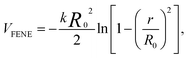 | (1) |
 | (2) |
We study chains of length 20, below the entanglement length, but long enough that chains have nearly Gaussian statistics. We use reduced units m = σ = ε = 1, where m is the monomer mass, length is in units of σ, time is in units of  and temperature is in units ε/kB where kB is Boltzmann's constant. For a polymer (like polystyrene) with Tg ≈ 100 °C, the reduced units can be mapped to physical units relevant to real polymer materials, where the size of a chain segments σ is typically about 1 nm to 2 nm, time is measured in ps, and ε ≈ 1 kJ mol−1.
For the NP, we use the model studied in ref. 5 and 6, in which the NP is built from a collection of 356 LJ particles bonded to form a large icosahedron. The outer shell of the icosahedron has 6 LJ particles along the edges, each separated by 21/6σ (the location of the LJ potential minimum), as illustrated in Fig. 1. This arrangement yields an icosahedron with edge length a = 5.61σ; for reference, a corresponding circumscribing sphere has radius 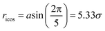 . Based on the unit mapping described above, this gives a scale of approximately 15 nm diameter for the NP. The NP size can be compared to the chain size by considering that the NP edge length is slightly larger than the average polymer end-to-end distance Re, which, at P = 1.0, ranges from 4.10 at low T = 0.45, to 4.25 at high T = 4.0. Such a polyhedral NP has a regular faceted shape that is somewhat similar to many metallic NPs or buckyballs, although we do not attempt to quantitatively match the energy scales of interactions with such NPs. To create a relatively stiff NP, each particle has mass mNP = 2.0 and is bonded to its ideal location in the icosahedral lattice via a FENE spring potential with a bond strength κNP = 45.0, and bond length R0 = 1.0. The strength of the LJ potential among the NP force sites is εpp = 2; between the NP force sites and monomers of the chains, we use the Lorentz–Berthelot mixing rules, so that
 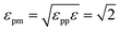 . See ref. 5 for additional technical description of the NPs used in our study.
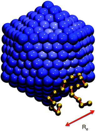 | ||
| Fig. 1 Snapshot of the model NP and a nearby polymer chain, which graphically shows that the NP size is commensurate with the chain size. The scale bar shows the mean end-to-end distance Re = 4.1σ at low T. | ||
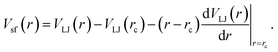
We investigate both attractive and excluded-volume only (or non-attractive) polymer NP interactions in order to distinguish the changes due to the steric constraints from those due to NP attraction. Monomers of chains and NP force sites interact via Vsf for attractive interaction; whereas for non-attractive interactions, the attractive r6 term of the VLJ is excluded as described in ref. 5.
We simulate a system of 100 chains of M = 20 monomers each for the pure melt, which we use as a basis to compare to the composite system. For the polymer–NP composite, we study systems with 800, 400, 200, or 100 chains (M = 20), which corresponds to NP concentrations ϕ = 0.0218, 0.0426, 0.0817, and 0.151, respectively. We only study the smallest ϕ = 0.0218 for attractive interactions. Equilibrium molecular simulations are performed along a path of constant pressure P = 1, which yields a T density of the pure polymer close to unity – the density studied previously.5 To increase simulation speed, we use the rRESPA multiple time step algorithm integration method34 with time step δt = 0.006, where forces are split into bonded and non-bonded components. At each T and ϕ studied, two equilibration runs were performed before the production runs: first the system is equilibrated at constant pressure P = 1.0 to compute the average density; we then further equilibrate at that average fixed density; finally, production runs occur at the same density. We follow this procedure so that the density of any run is fixed (as this simplifies analysis), but we also ensure that that 〈P〉 = 1.0. In other words, we follow an isobaric path. Equilibration and production times are chosen to exceed the characteristic relaxation time (see Section III) by roughly a factor 10 to avoid non-equilibrium effects. We study a wide range of temperatures, from highly non-Arrhenius (T = 0.45) to Arrhenius T ≳ 1.0. The temperature is controlled by the Nose–Hoover method.33
III. Effect of NP on melt dynamics
To evaluate changes to Tg and fragility, we examine the characteristic relaxation time with variable ϕ and T along an isobaric path, and compare those changes with previous results along an isochoric path.5,27 As a baseline for comparison, we first consider the pure melt (ϕ = 0) as a reference point. The structural relaxation of the melt can be characterized by the coherent intermediate scattering function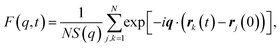 | (3) |
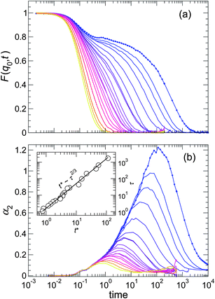 | ||
| Fig. 2 (a) Coherent scattering function F(q0,t) and (b) non-Gaussian parameter α2 for the pure melt. Temperature is indicated by the color gradient, which goes from blue at the lowest T – where relaxation is highly non-exponential – to yellow at a high T. The slowing relaxation of F(q0,t) is accompanied by a significant increase in the cooperativity of motion, as indicated by α2(t). The inset shows the “decoupling” of the characteristic times scales τ and t* of F(q0,t) and α2(t), respectively. | ||
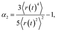
Since we also consider the cooperativity of motion, it is valuable to examine the non-Gaussian parameter α2,
 | (4) |
To characterize how NPs change the melt relaxation dynamics, we first consider how τ varies with ϕ and T as compared to the pure melt. Fig. 3 shows that τ increases with increasing ϕ for attractive NP interactions, consistent with earlier simulations performed isochorically.5,6 For non-attractive interactions, τ varies little from the pure system. In contrast, along an isochoric path, τ decreases significantly with increasing ϕ. We can reconcile this difference from the fact that the repulsive interaction have a “renormalizing” effect on the density far from the NP surface along an isobaric path. Specifically, far from the NP surface, ρ increases slightly relative to the pure system at the same T (discussed in the Appendix), which should cause τ to increase far from the NP surface; this increase counterbalances the expected decrease of τ near the NP surface – yielding almost no overall change. We analyze these competing effects in detail later in the spatial variation of relaxation time and cooperativity (Section V). This represents an important practical difference, since experiments are not normally conducted along fixed density paths.
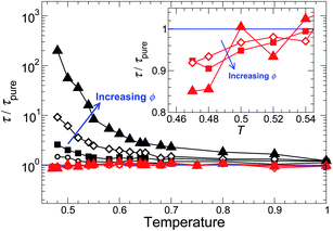 | ||
| Fig. 3 The relaxation time τ relative to the pure melt τpure for different NP concentrations. The black symbols are for attractive polymer–NP interactions, and the red symbols and solid lines are for a non-attractive polymer–surface interaction, where the effect on the melt dynamics is evidently weak. The symbol size is proportional to ϕ; specific symbols are ϕ = 0.0218 (○), 0.0426 (□), 0.0817 (◇), and 0.151 (△). The inset magnifies τ/τpure at the lowest T simulated for the non-attractive case, showing that there is a weak decrease of τ due to NP interactions. | ||
We use our data for τ to estimate the glass transition temperature Tg and the fragility of the glass formation by fitting τ(T) with the Vogel–Fulcher–Tamman40 equation
 | (5) |
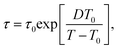
Consistent with the changes in τ, we find that Tg increases as ϕ increases for attractive polymer–NP interactions, as expected from earlier studies.5–7,16 For non-attractive polymer–NP interactions, the ϕ dependence of Tg is weak, which is expected since τ is nearly ϕ independent along our isobaric path; this contrasts the isochoric behavior, where Tg decreases with ϕ.
To quantify fragility, we primarily consider a common definition based on the logarithmic slope of relaxation near Tg,
 | (6) |
We estimate m using the same VFT fit to τ used to evaluate Tg. Fig. 4b shows that, like Tg, m increases as ϕ increases for attractive polymer–NP interactions (like isochoric results27); for non-attractive interactions, m shows no substantial change with ϕ, except at the largest ϕ where there is a small decrease in m – while isochoric results27 show a stronger decrease of m with ϕ. The fact that fragility changes are much weaker along isobaric paths means that, at small ϕ, changes in fragility are nearly undetectable. This is consistent with experiments,21 where there is no discernable fragility changes at small NP concentration (comparable to 1% by mass); these studies also had the complication that the NPs had polymer chains grafted onto their surface, an effect that may reduce the impact of NP on the melt. At larger NP concentrations, changes of fragility have been reported. Bansal et al.13 found that repulsive interactions caused Tg to decrease, accompanied by an appreciable broadening of the glass transition region, indicative of increased strength (decreased fragility) of glass formation. Cabral and co-workers22–24 reported behavior expected for attractive polymer–NP interactions, namely an increase in Tg, accompanied by an increased fragility for fullerenes is a polystyrene matrix. Notably, these effects disappeared when the particles exhibited appreciable aggregation, suggesting that the fragility change is a specifically nanostructural effect on the polymer melt dynamics.
 | ||
| Fig. 4 (a) Glass transition temperature Tg and (b) fragility m relative to the pure melt for both attractive and non-attractive NP interactions. The filled diamond symbols and dashed lines are for an isochoric approach to Tg,5,27 where the effect is more pronounced than along an isobaric path (circle symbols with solid line). The black symbols are for attractive NP interactions and the red symbols are for non-attractive NP interactions. The values presented are average values obtained by VFT fits using seven different T ranges of data that include or exclude points at the margins of the non-Arrhenius regime of τ. From these fits, we also obtain the uncertainties, which we show as error bars in the graph. | ||
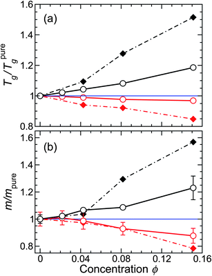
It is experimentally known that, for many polymers, m and Tg vary in an approximately proportional way;31 proportionality has also observed in our previous simulations of polymer composites along an isochoric path.27 Consequently, we check for such a possibility, and Fig. 5a confirms that the relative Tg and m for NP composites systems – both along isochoric and isobaric paths – vary proportionally. Moreover, by scaling these quantities relative to the pure melt, all data fall onto a single master line. However, recent simulations of thin polymer films using the same polymer model show that this proportionality can fail in very thin films.41 This demonstrates the limitations of using Tg as a predictor for fragility changes, and this finding also suggests that “mapping” between nanocomposites and thin films must be done with caution for ultra-thin films or large NP concentrations.
 | ||
| Fig. 5 (a) Parametric plot of relative fragility m/mpureTg/Tpureg. The isochoric data are normalized by the pure system at density ρ = 1; similarly, the isobaric data are normalized by the pure system at pressure P = 1. The dotted line is the best fit linear relation, showing an approximate proportionality for the range of NP concentrations and interactions investigated. (b) A similar plot showing the proportionality between Tg and the high-T activation energy Ea. | ||
A similar proportionality can be expected between Tg and the high temperature activation energy Ea for relaxation, since both should be proportional to the overall scale of cohesive interactions. We obtain Ea by fitting the high-T data to the Arrhenius form,
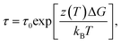
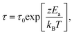
| τ = τ0exp[Ea/kBT]. | (7) |
We indeed find a proportionality between Tg and Ea is our isobaric simulations. We further check whether isochoric and isobaric data follow the same proportionality by scaling the quantities relative to the pure melt (Fig. 5b). A single relation captures the data reasonably well, but close inspection of it shows that the isobaric data may have a somewhat smaller scaled proportionality constant. The proportionality between Tg and Ea has important practical and conceptual consequences for quantifying fragility in relation to cooperative atomic motion, as we will discuss in the next section.
IV. Effect of NP on cooperative molecular rearrangement
A. Cooperativity and the Adam–Gibbs approach
A central challenge in describing glass formation is the origin of the rapidly increasing relaxation time approaching Tg. This is the defining characteristic of fragile glass-forming fluids. If one makes a natural assumption that relaxation is an activated processes, the Arrhenius form (eqn (7)) defines a generalized T-dependent activation energy| E(T) = T ln τ/τ0, | (8) |
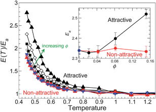 | ||
| Fig. 6 Temperature dependence of the activation energy E(T) (eqn (8)) normalized by the high-T limit Ea for all ϕ studied. Symbols are the same as Fig. 3, where black is for attractive NP–polymer interactions and red is for non-attractive NP–polymer interactions. The inset shows the values of the limiting high-T Arrhenius activation energy Ea as a function of ϕ, where the black symbols indicate attractive NP surface interactions, the red symbols indicate non-attractive NP surface interactions, and the blue symbols represent the pure polymer melt. | ||
A key element to explain the increase of E(T) is to recognize that such values cannot be readily reconciled on the basis of single particle motion. Indeed, on cooling, molecular motion becomes increasingly cooperative on time scales between the collision time and the relaxation time of the intermediate scattering function. A quantitative manifestation of such dynamical heterogeneity is that particle displacements are not Gaussian on these time scales,42–44 as already shown by the non-Gaussian parameter α2 (Fig. 2b). The concept of dynamical heterogeneity is the foundation of the Adam and Gibbs theory (AG) in which hypothetical cooperative rearranging regions (CRR) govern the energy barrier height for liquid relaxation. Specifically, AG hypothesized that the activation free energy is extensive in the size of z of CRR, resulting in a simple expression relating the structural relaxation time τ to the extent of collective motion,
 | (9) |
Unfortunately, AG offered no prescription for how to define the abstract CRRs from a molecular or particle perspective. Fortunately, the intervening years have offered a more quantitative view on the nature of cooperativity. In particular, simulations30,45–50,82 and colloidal experiments51–53 have both consistently shown that highly mobile particles typically move in a cooperative, string-like fashion that peaks on a time scale similar to t*. At larger time scales, cooperative motion takes a more compact, less elongated form.54 Previously, it was shown that the characteristic peak string size L* can be used as a proportional measure of z along an isochoric path of glass-formation for the same polymer–NP model.27 Below, we check the generalization of the former observations for an isobaric path, and also consider a generalization of the activation free energy proposed by AG.
To quantify the effects of NPs on cooperative dynamics, we evaluate the string-like motion of the most mobile particles following the methods established in previous work.30,45 We provide an illustration of the resulting strings in shown in Fig. 7, which qualitatively shows how the strings themselves tend the cluster. We show a representative example of the time and T dependence of the average string size 〈L(t)〉 for ϕ = 0.02 in Fig. 8. At each temperature, 〈L(t)〉 exhibits a characteristic peak string size L*, which increases as T decreases. The characteristic time at which 〈L(t)〉 exhibits a maximum also grows on cooling, and is similar to t* from α2(t). Additionally, the inset of Fig. 8 shows that the distribution P(T) taken at the time of the of the peak 〈L(t)〉 is exponential, as expected from dynamical polymerization models.55 Notably, this cooperative motion is largely insensitive to chain connectivity, so this type of collective motion should not be confused with reptation, where the chains are thought to move preferentially along their backbone coordinates.56
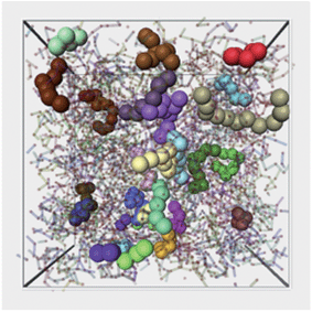 | ||
| Fig. 7 Illustration of a typical configuration of string-like cooperative regions for the time interval when 〈L(t)〉 is maximal. Each string is shown by large spheres in a different color. The polymer melt is also shown transparent. For purposes of the clarity, we only render strings of length larger than 4. | ||
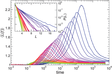 | ||
| Fig. 8 A representative sample of the mean string size 〈L(t)〉 for all T simulated at NP concentration ϕ = 0.02 with attractive polymer–NP interactions. The color gradient goes from yellow at highest T to blue at lowest T. The inset shows that the probability distribution P(L) taken at the time of the maximal 〈L(t)〉 for all the range of T simulated is exponential. | ||
From the behavior of 〈L(t)〉, we extract the characteristic peak L* for all systems studied, and also normalize L* relative to that of the pure reference system, as shown in Fig. 9. L* increases as the NP concentration ϕ increases for attractive interactions (like isochoric conditions), but we find a rather small change for non-attractive interactions (unlike isochoric conditions, where L* is significantly reduced). This difference is consistent with our previous observation that τ is only weakly affected at fixed pressure for non-attractive interactions. Thus, the effects of the NPs on cooperativity of segmental motion along an isobaric path are broadly consistent with those found isochorically.
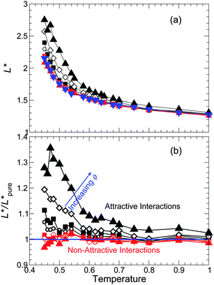 | ||
| Fig. 9 (a) The characteristic string size L* from the peak of 〈L(t)〉, and (b) relative to the pure melt, for all T, ϕ, and NP interactions simulated. L* for non-attractive NP interactions are nearly the same as the pure melt for all ϕ and T, as is the case for τ. Symbols are the same as Fig. 3. Generally, the behavior of L* in (a) is comparable to that of E(T) (see Fig. 6). Similarly, the behavior of L*/L*pure in (b) is comparable to that of ln τ/τpure (see Fig. 3). | ||
Consistent with the idea that L* may quantify the size z of CRR, the scale of the increase of L* on cooling is similar to the scale of the increase in the activation barrier E(T) (compare Fig. 9a with Fig. 6). Given the broad qualitative agreement, we quantitatively test eqn (9), where we identify L with the CRR size z. As stated above, it is normally assumed that ΔG is independent of T, i.e. ΔG is purely enthalpic. The applicability of AG to hard sphere simulations,57–59 where energy plays no role, calls this assumption into question. From thermodynamics and transition state theory60–62 we more generally expect a free energy of activation,
| ΔG = ΔH − TΔS, | (10) |
 | (11) |
Alternatively, one might consider that the barrier changes are primarily entropic in nature rather than enthalpic, so that ΔS is the dominant contribution.63–68 In such a case, eqn (9) reduces to a distinct relationship,
 | (12) |
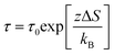
We test the traditional enthalpy dominated AG expression (eqn (11)) in Fig. 10a, using the previous results for Ea (Fig. 6 inset), so that no fit parameter is needed. We find that this form exhibits modest curvature for the present results; this curvature would not change if Ea were taken as a free parameter, since Ea determines slope, not curvature. In contrast the entropy dominated form (eqn (12)), shown in Fig. 10b, shows relatively less curvature, suggesting that the entropy term is the dominant contribution for low T at constant pressure in this system. Since ΔS is not known a priori, it is treated as a fit parameter. These observations mean that previous examinations of AG theory may need to be reassessed, since it is normal to simply assume that the ΔG is entirely enthalpic.
 | ||
| Fig. 10 Check of the Adam–Gibbs relation, assuming L represents the size of CRR. We consider two extreme cases where the activation free energy is dominated either by (a) the enthalpic contribution ΔH = Ea (eqn (11)) or (b) an entropic contribution δS (eqn (12)). For the enthalpy dominated case, Ea is obtained from the high T Arrhenius behavior (Fig. 6). In both cases, the data from low T (where τ varies most strongly) dominates. | ||
There are general theoretical reasons that we might expect ΔS to be the dominant term in eqn (9) and (10). Dyre and coworkers argued, in effect but not explicitly, that scaling consistency requires ΔG to be purely entropic for fluids interacting with purely repulsive power-law interactions, which they further argue is the predominant interaction in many van der Waals liquids.69,70 Consequently, they have criticized the general use of eqn (11) for molecular fluids with van der Waals interactions. By extension their reasoning also excludes the Arrhenius temperature at high temperatures, which itself lacks a rigorous theoretical foundation. It seems ironic that the original observations71 that stimulated Adam–Gibbs to develop their theory were empirically fit by the equivalent of eqn (12).
B. Cooperativity and fragility
Consistency of the string size with the AG expression has important implications for the molecular scale interpretation of fragility. Specifically, combining eqn (6), (9) and (10) yields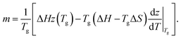 | (13) |
Considering the enthalpy dominated case where ΔG ≈ Ea, reduces eqn (13) to
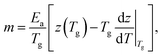 | (14) |
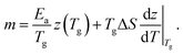 | (15) |
Again, the differential change of z is the dominant contribution, so that m ≈ TgΔSdz/dT|Tg.
Whether enthalpy or entropy dominated, the empirical proportionality of m, Tg, and Ea leads to a great simplification in the description of dynamics in the AG formulation. This proportionality applies to a significant class of materials (metallic glasses, polymer glasses with simple van der Waals interactions).31 In particular, a proportionality of m and Tg requires that the product DT0 in the VFT equation is constant, thereby reducing the number of free parameters. This means that τ (and presumably viscosity) only depend on the difference of temperature between T and T0 (effectively Tg).27 The proportionality between Tg and m in the VFT equation also leads to the Williams–Landel–Ferry equation72, and explains its ‘universal’ parameter values for polymer materials.
It must be appreciated that there are materials for which the proportionality between m and Tg does not hold, particularly materials for which the cohesive interaction strength is highly variable.73,74 In these enthalpically dominated systems, m more significantly affected by the strength of the interactions than to the collective dynamics. Under these circumstances we can define a measure of molecular cooperativity,
 | (16) |
Comparing with eqn (14), it is apparent that c should capture the extent of cooperativity, which we expect has significance to other features commonly associated with collective motion in glass-forming liquids (such as the decoupling of diffusion and relaxation and the stretching exponent describing the long time decay of F(q,t)). This measure of cooperative motion also emphasizes the necessity of determining both m and Tg in characterizing the glass transition.
V. Spatial variation of relaxation and fragility
In this section, we take advantage of the fact that our simulations allow us to explicitly examine the spatial variation of relaxation, so that we can understand to what degree changes in the rate of relaxation in the nanocomposites can be attributed to interfacial effects. Since the previously examined coherent scatting function is inherently non-local, we use the self-part of F(q0,t) (eqn (3)) with j = k, which can be partitioned into the contribution based on the position of a monomer at t = 0. Consequently, we can evaluate the relaxation time τ(r) as a function of distance r from the NP surface.
Fig. 11a shows that for attractive polymer–NP interaction, τ(r) grows approaching the NP–polymer surface, while τ(r) decreases approaching the NP surface for non-attractive polymer–NP interactions. In other words, the attractive surface slows the monomer mobility, while non-attractive interactions enhance relaxation. This spatial dependence of τ(r) is consistent with previous isochoric studies5,6 and thin film studies.7,16 For attractive NP surface interactions, τ(r) is nearly ϕ independent at a low ϕ; at the largest ϕ, τ(r) increases relative to its value at smaller ϕ. For non-attractive interactions, we see that τ(r) increases as ϕ increases. Significantly, τ(r) far from the NP surface does not converge to the value of the pure melt. Instead, the asymptotic value of τ is slightly larger than that of the pure melt. The increase of τ far from the NP can be attributed to the fact that the asymptotic density ![[small rho, Greek, macron]](https://www.rsc.org/images/entities/i_char_e0d1.gif) a far from the NP is larger than the pure polymer melt (see the Appendix). This is unlike the isochoric studies,5,6 where the density far from the NP is engineered to match the pure melt, eliminating this effect. In this sense, there are important non-local effects of the NP on polymer packing that impact the overall relaxation behavior of the composite. This is particularly noticeable for the case of non-attractive interactions, as the decrease in τ near the NP surface and the increase far from the surface compensate to yield nearly no change in the overall rate of relaxation. Hence, the fact that τ is nearly unchanged on average for non-attractive interactions does not indicate that τ is unchanged near the surfaces.
a far from the NP is larger than the pure polymer melt (see the Appendix). This is unlike the isochoric studies,5,6 where the density far from the NP is engineered to match the pure melt, eliminating this effect. In this sense, there are important non-local effects of the NP on polymer packing that impact the overall relaxation behavior of the composite. This is particularly noticeable for the case of non-attractive interactions, as the decrease in τ near the NP surface and the increase far from the surface compensate to yield nearly no change in the overall rate of relaxation. Hence, the fact that τ is nearly unchanged on average for non-attractive interactions does not indicate that τ is unchanged near the surfaces.
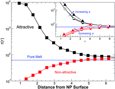 | ||
| Fig. 11 The relaxation time τ from the self-intermediate scattering function as a function of distance from NP surface for a representative ϕ = 0.04 at T = 0.50. The inset shows various ϕ for the same T. | ||
To complement the spatial variation of τ(r), Fig. 12 shows the T dependence of τ(T) for both attractive and non-attractive polymer–NP interactions at various distances from the NP surface. We see that the T-dependence of τ differs from near to far from the NP – but the fragility change is harder to discern, since fragility includes both T-dependence and the relative Tg values, which both change simulataneously. Accordingly, the spatial variation of τ is more conveniently parameterized by evaluating the spatial dependence of Tg and m as a function of r. To evaluate Tg(r) and m(r), we fit the behavior of τ(r,T) for various distances to the VFT form (eqn (5)), following the same approach used for the system average.
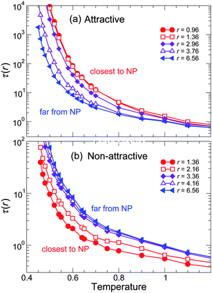 | ||
| Fig. 12 Temperature dependence of the relaxation time τ for (a) attractive and (b) non-attractive interactions at various distances r from NP surface for representative ϕ = 0.04. The color gradient goes from blue for the furthest distance from NP surface to red for the closest distance to the NP surface. From these data we can extract Tg(r) and m(r), shown in the subsequent figure. | ||
For attractive polymer–NP interactions, Fig. 13 shows that Tg(r) increases approaching the NP surface, consistent with the behavior of τ(r) of the pure melt. Moreover, note that Tg(r) is larger than that of the pure melt even at the largest distances, similar to τ(r). Based on the observed proportionality between Tg and m for the NP system as a whole, one would anticipate that m(r) should also increase approaching the NP surface. However, we find that m(r) instead decreases approaching the NP surface. We can rationalize the decrease of m(r) near the NP surface from packing considerations. Specifically, the attractive polymer–NP interactions favor enhanced monomer packing approaching the NP, and improved packing should lead to a decrease of fragility.75 However, for the monomers immediately at the NP surface, monomer packing is frustrated (even with attractive interactions) due to the NP shape. Consequently, m(r) at the closest distance from the NP surface approximately saturates.
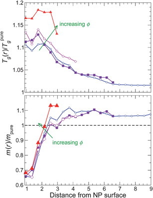 | ||
| Fig. 13 The glass transition temperature Tg and fragility m for attractive NP surface interaction as a function of distance from the NP surface. The color gradient goes from blue at the lowest NP concentration to red at the highest NP concentration. | ||
Such an opposing trend in fragility and Tg has also been observed in measurements on thin polymer films76. But this leaves the question: how can m as a whole increase while m near the surface decreases? This paradox is resolved by recognizing that m far from the NP increases relative to the pure melt. In fact, both m and Tg far from the NP surface are larger than the pure melt values, and this asymptotic behavior dominates the system mean (since large distances are dominant when spherically averaging). This increase at large r is consistent with the change in density far from the surface relative to the pure melt. This complication does not occur for the previous isochoric data.5
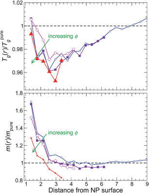
We next examine the behavior of Tg(r) and m(r) for non-attractive NP interactions (Fig. 14). The spatial dependence of Tg(r) mirrors that of τ(r), except very near to the NP surface. The difference between τ(r) and Tg(r) near the surface is connected with the spatial variation of the fragility. Specifically, the fragility m(r) increases significantly approaching the NP surface. Consequently, for T lower than we can simulate, τ near the surface must then exceed τ at larger distance, which will lead to a relative increase Tg near the surface. The increase of m(r) near the surface can be understood by fact that the NP repulsion frustrates the monomer packing near the NP, and such packing frustration has been shown to lead to an increase in fragility.75
 | ||
| Fig. 14 The glass transition temperature Tg and fragility m for non-attractive NP surface interaction as a function of distance from the NP surface. The color gradient goes from blue at the lowest NP concentration to red at the highest NP concentration. | ||
Comparing the behavior of Tg(r) and m(r) for non-attractive NP interactions, these quantities appear more closely coupled (like the pure melt) than for attractive interactions. However, based on our findings, the simple proportionality between Tg and m is not robust when we attempt to apply this concept locally.
The ϕ dependence of Tg(r) and m(r) are also informative. In particular, if we adopt ideas from the thin film literature,7,77,78 one might expect a “layer” picture of dynamics where the addition of NP only perturb surface behavior. In this case, the effect of concentration (playing the role of thickness in films) serves only to weight the contribution of surface versus bulk behavior, so that Tg(r) and m(r) are independent of ϕ. Indeed, for small ϕ, Tg(r) and m(r) are nearly ϕ independent for both interaction types. However, Tg(r) clearly differs at the largest ϕ. This suggests that there are important effects of the confinement between NP that go beyond surface interactions when the concentration is large enough. Similar behavior in films at very small thickness has also been seen using the same polymer model.41
VI. Discussion and conclusions
We have examined the inter-relations between changes of Tg, fragility, and cooperative motion caused by an ideal dispersion of NP in a simple model polymer melt, and contrasted the behavior of isochoric and isobaric approaches to Tg. We found that the behavior along either thermodynamic path is qualitatively similar. However, it is significant that along isobaric paths the quantitative scale of changes is reduced, so that the effects at small NP concentrations can sometimes be difficult to discern from the pure melt. In addition, at small NP concentration, the effects of Tg and fragility are proportional – at least on average. From a practical point of view, it means that under limited circumstances, only one quantity is needed to predict both Tg and fragility changes. However, we see that this simple proportionality fails when structural relaxation is probed at a segmental scale.Our findings for Tg and fragility are based on the relaxation probed at the monomer (or segmental) scale, and the effect of NP on relaxation can be scale dependent. In particular, ref. 24 found that fragility on the segment scale differs from that of the chain scale in a C60 nanocomposite. Therefore, we evaluate τ for an alternate q-vector on the scale of polymer chains q = 2π/Rg to check for such an effect. Fig. 15 shows the resulting behaviors of Tg and fragility as a function of NP concentration at the chain scale. The trends of Tg for the attractive and non-attractive NP systems at the chain scale are indeed similar to that of the monomer scale. However, the behavior of the fragility at the chain scale is noticeable different. Firstly, both attractive and non-attractive systems show a decrease in fragility with increasing concentration at the chain scale. Additionally, for attractive NP interactions the fragility is smaller than that of the non-attractive NP interactions, opposite to the trend at monomer scales. Apparently, it is important to separately examine fragility at chain scales, a topic for future studies.
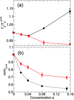 | ||
| Fig. 15 (a) Glass transition temperature Tg and (b) fragility m relative to the pure melt for both attractive and non-attractive NP interactions at the scale of polymer chains. This figure should be compared with Fig. 4, which examines the same behavior at the monomer scale. The black symbols are for attractive NP interactions and the red symbols are for non-attractive NP interactions. Uncertainties are determined using the same approach as those in Fig. 4. | ||
Given the success is relating changes in relaxation to the scale of cooperative motion for the system as a whole in the framework of the AG theory, it would seem natural to probe for such a relation at a segmental scale. Specifically, can we relate the changes in τ(r) as a function of distance from the NP surface with a changes in the local scale L of cooperative motion? The problem with such a question is that the cooperative motion is an inherently non-local phenomenon, so that attempts to define an appropriate local L(r) do not readily conform the expected limiting behavior. Similarly, the configurational entropy (which should be proportional to L−1 according to AG) is both practically and conceptually difficult to define in a local manner.
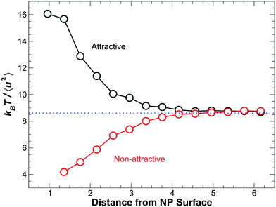
A possible alternative route to relate spatial variation of the relaxation time to structural quantities is through the Debye–Waller factor (DWF) 〈u2〉, which measures the amplitude of vibrational rattling related to the cage size. From a structural standpoint, it has been argued that kT/〈u2〉 can be interpreted as a measure of local stiffness or modulus,28 which can also be expected to impact τ. As a preliminary test, we have examined the spatial dependence 〈u2〉. Formally, the DWF can be defined as 〈u2〉 = 〈r2(t0)〉, where t0 is the time of the crossover from the ballistic motion to cage motion of the mean square displacement r2(t); following ref. 79, we take t0 = 1.1, corresponding to a time on the order of 1 ps in non-reduced time units. Fig. 16 shows that kT/〈u2〉 increases approaching the attractive NP surface, consistent with the behavior of τ(r). Similarly, for monomers near the non-attractive NP surface, kT/〈u2〉 decreases approaching the NP surface. Given this qualitative similarity, further examination of the relation between τ and 〈u2〉 will be considered systematically in future work.
 | ||
| Fig. 16 The inverse of the Debye–Waller factor 〈u2〉 as a function of distance from NP surface at temperature for ϕ = 0.04 at T = 0.50. Black symbols and dashed lines represent attractive interactions. Red symbols represent non-attractive interactions. This behavior is qualitatively matches that of the distance dependence of the structural relaxation time τ shown in Fig. 11, which is for the same system. Establishing a quantitative relationship is a goal of future work on our nanocomposites. Note that an inversion of this effect is possible for T < Tg.80 | ||
The pursuit of this problem will first require an assessment of the relation between τ and 〈u2〉 to determine if the universal relation proposed by ref. 81,83 (or some other relation) can adequately describe our data covering a large range of fragility. If such a relation could be found, then we would be a in a good position to map a local short time property that can reliably inform about variations in the local mobility in the nanocomposite. Additionally, the DWF has the advantage that it is experimentally accessible via neutron scattering, while experimental measurement of string size is typically limited to colloidal systems where direct video microscopy is possible.
Finally, we mention some other topics that merit future study. First, fragility may also be significantly affected by NP size. For example, ref. 28 saw that the direction of the effect on Tg and m of the melt can be opposite to that of adding NP for a solvent with attractive interaction that was smaller than the statistical segment unit of the polymer beads. Thus, the reversal of effects upon going from solvent to NP requires systematic investigation. Additionally, NP clustering must have dramatic effects, but this is far more challenging to effectively simulate. The effect of NPs on the high frequency shear modulus is important to investigate to understand how these particles alter the shear viscosity of the nanocomposite melts. It may also be valuable to study how the rigidity of the NP affects changes of Tg and the fragility of the nanocomposite, since many NP have ‘soft’ grafted polymer layers to help disperse them in polymer matrices. We anticipate that the NP stiffness is a relevant factor, since it should alter the local molecular packing of the polymers and thus alter the fragility of the nanocomposite.
VII. Appendix: effect of NP on melt density
At constant pressure, the addition of NP particles changes the local and overall density of the melt and it is natural to consider these density changes relate to mobility changes in the melt based on the attractive idea of free volume theory, which postulates higher mobility goes hand in hand with lower density. As we shall see, these changes depend on both the NP–polymer interaction and NP volume fraction ϕ. We show the dependence of the monomer density ρ(r) on the distance r from the NP surface in Fig. 17a for attractive polymer–NP interactions. The monomers form “layers” near the NP surface due to packing constraints. A similar layering occurs for non-attractive interactions, as illustrated in Fig. 17b, although there is not a specifically preferred distance for the first layer (see ref. 5 for a detailed discussion). An important observation to take away from these data is that density near the NP surface is increased near the surface for both attractive and non-attractive interactions. In a simple free volume picture of the dynamics, the enhancement of density near the NP surface would lead to slowed relaxation. Instead, we have seen that the relaxation can be enhanced or reduced near the NP surface, depending on interactions. Consequently, such a free volume approach is inadequate to describe the observed changes in dynamics.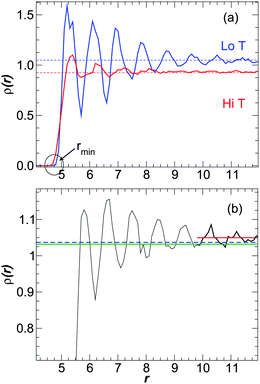 | ||
| Fig. 17 (a) Density ρ(r) as a function of the distance r from the NP surface for attractive polymer–NP interactions at ϕ = 0.02. The blue line shows ρ(r) at T = 0.45, and the red solid line shows ρ(r) at T = 0.9. The horizontal dashed lines shows the average density for each T (not the density of the pure melt), computed as explained in the text. (b) Density ρ(r) as a function of the distance r from the NP surface for non-attractive polymer–NP interactions ϕ = 0.02 at T = 0.45. The blue dashed line shows ρ for the pure melt, the green line shows , and the red line shows the asymptotic a, indicating that a > ρpure > . | ||
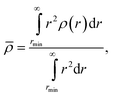
Since ρ(r) varies with r, we define a overall density for each system by the integral of the density profile
 | (17) |
can differ significantly from the asymptotic value of density a far from the NP (Fig. 17b). The asymptotic value ρa is the value that can be more readily compared to ρ of the pure melt. We compute ρa by taking the average of density in the outer most layers. Attractive and non-attractive the NP surface interactions systems are asymptotically denser than the pure melt at any ϕ. Fig. 18b suggests that the NP presence induces an increase in the asymptotic density for both attractive and non-attractive NP surfaces. Since ρa increases monotonically for attractive interactions and decreases for non-attractive NP interactions as ϕ increases, the increasing or decreasing behavior depends on the NP interaction.
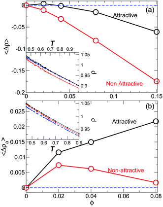 | ||
| Fig. 18 (a) The average density difference 〈Δρ〉 relative to the pure system as a function of concentration ϕ for attractive and non-attractive NP interactions. The inset shows the temperature dependence of the density ρ(T), revealing that the density shift is nearly T-independent. (b) The average difference in the asymptotic density 〈Δρa〉 relative to the pure system for attractive and non-attractive NP interactions. The inset shows the temperature dependence of the density ρ(T) where the shift is also nearly T-independent. For both graphs: the blue dashed line is for the pure system, the black solid line correspond to attractive NP surface interaction, and the red solid line correspond to non-attractive NP surface interaction at ϕ = 0.02. Due to the small number of layers for ϕ = 0.15, we only compute ρa for ϕ < 0.15. | ||
Acknowledgements
JFD acknowledges support from NIH grant 1 R01 EB006398-01A1. BAPB and FWS acknowledge support from NSF grant number CNS-0959856 and ACS-PRF grant 51983-ND7.References
- J. Jancar, J. F. Douglas, F. W. Starr, S. K. Kumar, P. Cassagnau, A. J. Lesser, S. S. Sternstein and M. J. Buehler, Polymer, 2010, 51, 3321–3343 CrossRef CAS.
- K. I. Winey and R. A. Vaia, MRS Bull., 2007, 32, 314–319 CAS.
- G. Schmidt and M. Malwitz, Curr. Opin. Colloid Interface Sci., 2003, 8, 103–108 CrossRef CAS.
- A. C. Balazs, T. Emrick and T. P. Russell, Science, 2006, 314, 1107–1110 CrossRef CAS.
- F. W. Starr, T. B. Schroder and S. C. Glotzer, Macromolecules, 2002, 35, 4481–4492 CrossRef CAS.
- F. W. Starr, T. B. Schrøder and S. C. Glotzer, Phys. Rev. E, 2001, 64, 021802 CrossRef CAS.
- J. A. Torres, P. F. Nealey and J. J. de Pablo, Phys. Rev. Lett., 2000, 85, 3221–3224 CrossRef CAS.
- G. Smith, D. Bedrov and O. Borodin, Phys. Rev. Lett., 2003, 90, 226103 CrossRef.
- V. Arrighi, I. McEwen, H. Qian and M. Prieto, Polymer, 2003, 44, 6259–6266 CrossRef CAS.
- H. Montes, F. Lequeux and J. Berriot, Macromolecules, 2003, 36, 8107–8118 CrossRef CAS.
- M. E. Mackay, T. T. Dao, A. Tuteja, D. L. Ho, B. V. Horn, H. Kim and C. J. Hawker, Nat. Mater., 2003, 2, 762–766 CrossRef CAS.
- T. Desai, P. Keblinski and S. Kumar, J. Chem. Phys., 2005, 122, 134910 CrossRef.
- A. Bansal, H. Yang, C. Li, K. Cho, B. C. Benicewicz, S. K. Kumar and L. S. Schadler, Nat. Mater., 2005, 4, 693–698 CrossRef CAS.
- M. Alcoutlabi and G. McKenna, J. Phys.: Condens. Matter, 2005, 17, R461–R524 CrossRef CAS.
- D. Fragiadakis, P. Pissis and L. Bokobza, Polymer, 2005, 46, 6001–6008 CrossRef CAS.
- J. Baschnagel and F. Varnik, J. Phys.: Condens. Matter, 2005, 17, R851–R953 CrossRef CAS.
- P. Rittigstein and J. M. Torkelson, J. Polym. Sci., Part B: Polym. Phys., 2006, 44, 2935–2943 CrossRef CAS.
- K. Nusser, G. J. Schneider, W. Pyckhout-Hintzen and D. Richter, Macromolecules, 2011, 44, 7820–7830 CrossRef CAS.
- B. J. Anderson and C. F. Zukoski, Langmuir, 2010, 26, 8709–8720 CrossRef CAS.
- S. Y. Kim and C. F. Zukoski, Soft Matter, 2012, 8, 1801–1810 RSC.
- O. Hyunjoon and P. F. Green, Nat. Mater., 2009, 8, 139–143 CrossRef CAS.
- H. C. Wong, A. Sanz, J. F. Douglas and J. T. Cabral, J. Mol. Liq., 2010, 153, 79–87 CrossRef CAS.
- A. Sanz, M. Ruppel, J. F. Douglas and J. T. Cabral, J. Phys.: Condens. Matter, 2008, 20, 104209 CrossRef.
- Y. Ding, S. Pawlus, A. P. Sokolov, J. F. Douglas, A. Karim and C. L. Soles, Macromolecules, 2009, 42, 3201–3206 Search PubMed.
- G. J. Papakonstantopoulos, K. Yoshimoto, M. Doxastakis, P. F. Nealey and J. J. de Pablo, Phys. Rev. E: Stat., Nonlinear, Soft Matter Phys., 2005, 72, 031801 CrossRef.
- G. J. Papakonstantopoulos, M. Doxastakis, P. F. Nealey, J.-L. Barrat and J. J. de Pablo, Phys. Rev. E: Stat., Nonlinear, Soft Matter Phys., 2007, 75, 031803 CrossRef.
- F. W. Starr and J. F. Douglas, Phys. Rev. Lett., 2011, 106, 115702 CrossRef.
- R. A. Riggleman, J. F. Douglas and J. J. de Pablo, J. Chem. Phys., 2007, 126, 234903 CrossRef.
- G. Adam and J. H. Gibbs, J. Chem. Phys., 1965, 43, 139–146 CrossRef CAS.
- C. Donati, J. F. Douglas, W. Kob, S. J. Plimpton, P. H. Poole and S. C. Glotzer, Phys. Rev. Lett., 1998, 80, 2338–2341 CrossRef CAS.
- Q. Qin and G. B. McKenna, J. Non-Cryst. Solids, 2006, 352, 2977–2985 Search PubMed.
- G. S. Grest and K. Kremer, Phys. Rev. A: At., Mol., Opt. Phys., 1986, 33, 3628–3631 CrossRef CAS.
- M. P. Allen and D. J. Tildesley, Computer Simulation of Liquids, Oxford University Press, Oxford, 1987 Search PubMed.
- M. Tuckerman, B. J. Berne and G. J. Martyna, J. Chem. Phys., 1992, 97, 1990–2001 CrossRef CAS.
- M. Aichele and J. Baschnagel, Eur. Phys. J. E: Soft Matter Biol. Phys., 2001, 5, 229–243 Search PubMed.
- M. D. Ediger, Annu. Rev. Phys. Chem., 2000, 51, 99–128 CrossRef CAS.
- R. Richert, J. Phys.: Condens. Matter, 2002, 14, R703–R738 CrossRef CAS.
- C. Donati, S. C. Glotzer, P. H. Poole, W. Kob and S. J. Plimpton, Phys. Rev. E: Stat. Phys., Plasmas, Fluids, Relat. Interdiscip. Top., 1999, 60, 3107–3119 CrossRef CAS.
- W. Kob and H. C. Andersen, Phys. Rev. E: Stat. Phys., Plasmas, Fluids, Relat. Interdiscip. Top., 1995, 51, 4626–4641 CrossRef CAS.
- C. A. Angell, Science, 1995, 267, 1924–1935 CrossRef CAS.
- P. Z. Hanakata, J. F. Douglas and F. W. Starr, J. Chem. Phys., under review Search PubMed.
- T. Odagaki and Y. Hiwatari, Phys. Rev. A: At., Mol., Opt. Phys., 1991, 43, 1103–1106 Search PubMed.
- W. Kob, C. Donati, S. J. Plimpton, P. H. Poole and S. C. Glotzer, Phys. Rev. Lett., 1997, 79, 2827–2830 CrossRef CAS.
- M. S. Shell, P. G. Debenedetti and F. H. Stillinger, J. Phys.: Condens. Matter, 2005, 17, S4035 CrossRef CAS.
- M. Aichele, Y. Gebremichael, F. W. Starr, J. Baschnagel and S. C. Glotzer, J. Chem. Phys., 2003, 119, 5290–5304 Search PubMed.
- Y. Gebremichael, M. Vogel and S. Glotzer, J. Chem. Phys., 2004, 120, 4415–4427 Search PubMed.
- R. A. Riggleman, K. Yoshimoto, J. F. Douglas and J. J. de Pablo, Phys. Rev. Lett., 2006, 97, 045502 CrossRef.
- M. Vogel, B. Doliwa, A. Heuer and S. Glotzer, J. Chem. Phys., 2004, 120, 4404–4414 Search PubMed.
- T. Schroder, S. Sastry, J. Dyre and S. Glotzer, J. Chem. Phys., 2000, 112, 9834–9840 CrossRef CAS.
- N. Giovambattista, F. W. Starr, F. Sciortino, S. V. Buldyrev and H. E. Stanley, Phys. Rev. E, 2002, 65, 041502 Search PubMed.
- Z. Zheng, F. Wang and Y. Han, Phys. Rev. Lett., 2011, 107, 065702 CrossRef.
- Z. Zhang, P. J. Yunker, P. Habdas and A. G. Yodh, Phys. Rev. Lett., 2011, 107, 208303 Search PubMed.
- E. R. Weeks, J. C. Crocker, A. C. Levitt, A. Schofield and D. A. Weitz, Science, 2000, 287, 627–631 CrossRef CAS.
- P. Chaudhuri, S. Sastry and W. Kob, Phys. Rev. Lett., 2008, 101, 190601 Search PubMed.
- J. F. Douglas, J. Dudowicz and K. F. Freed, J. Chem. Phys., 2006, 125, 144907 CrossRef.
- D. Masao and S. F. Edwards, The Theory of Polymer Dynamics, Oxford University Press, Oxford, 1988 Search PubMed.
- R. J. Speedy, J. Chem. Phys., 1999, 110, 4559–4565 CrossRef CAS.
- R. J. Speedy, J. Chem. Phys., 2001, 114, 9069–9074 Search PubMed.
- L. Angelani and G. Foffi, J. Phys.: Condens. Matter, 2007, 19, 256207 Search PubMed.
- J. F. Kincaid, H. Eyring and A. E. Stearn, Chem. Rev., 1941, 28, 301–365 Search PubMed.
- R. M. Barrer, Trans. Faraday Soc., 1943, 39, 48–59 RSC.
- L. Qun-Fang, H. Yu-Chun and L. Rui-Sen, Fluid Phase Equilib., 1997, 140, 221–231 Search PubMed.
- Y. Rosenfeld, Chem. Phys. Lett., 1977, 48, 467–468 Search PubMed.
- Y. Rosenfeld, Phys. Rev. A: At., Mol., Opt. Phys., 1977, 15, 2545–2549 CrossRef.
- Y. Rosenfeld, J. Phys.: Condens. Matter, 1999, 11, 5415 CrossRef CAS.
- J. Mittal, J. R. Errington and T. M. Truskett, Phys. Rev. Lett., 2006, 96, 177804 CrossRef.
- R. Grover, W. G. Hoover and B. Moran, J. Chem. Phys., 1985, 83, 1255–1259 Search PubMed.
- M. Dzugutov, Nature, 1996, 381, 137–139 CrossRef CAS.
- J. C. Dyre, T. Hechsher and K. Niss, J. Non-Cryst. Solids, 2009, 355, 624–627 Search PubMed.
- N. Gnan, T. B. Schroder, U. R. Pedersen, N. P. Bailey and J. C. Dyre, J. Chem. Phys., 2009, 131, 234504 CrossRef.
- A. B. Bestul and S. S. Chang, J. Chem. Phys., 1964, 40, 3731–3733 Search PubMed.
- M. L. Williams, R. F. Landel and J. D. Ferry, J. Am. Chem. Soc., 1955, 77, 3701–3707 CrossRef CAS.
- D. Fragiadakis, S. Dou, R. H. Colby and J. Runt, J. Chem. Phys., 2009, 130, 064907 Search PubMed.
- E. B. Stukalin, J. F. Douglas and K. F. Freed, J. Chem. Phys., 2009, 131, 114905–114913 CrossRef.
- J. Dudowicz, K. F. Freed and J. F. Douglas, Adv. Chem. Phys., 2008, 137, 125–222 CAS.
- S. Kim, M. K. Mundra, C. B. Roth and J. M. Torkelson, Macromolecules, 2010, 43, 5158–5161 Search PubMed.
- J. L. Keddie, R. A. L. Jones and R. A. Cory, Faraday Discuss., 1994, 98, 219–230 RSC.
- J. A. Forrest, K. Dalnoki-Veress and J. R. Dutcher, Phys. Rev. E: Stat. Phys., Plasmas, Fluids, Relat. Interdiscip. Top., 1997, 56, 5705–5716 CrossRef CAS.
- F. W. Starr, S. Sastry, J. F. Douglas and S. C. Glotzer, Phys. Rev. Lett., 2002, 89, 125501 CrossRef.
- T. E. Dirama, J. E. Curtis, G. A. Carri and A. P. Sokolov, J. Chem. Phys., 2006, 124, 034901 CrossRef.
- L. Larini, A. Ottochian, C. De Michele and D. Leporini, Nat. Phys., 2008, 4, 42–45 CrossRef CAS.
- F. Puosi and D. Leporini, J. Chem. Phys., 2012, 136, 164901 Search PubMed.
- A. Ottochian and D. Leporini, J. Non-Cryst. Solids, 2011, 357, 298–301 CrossRef CAS.
Footnote |
| † Official contribution of the U.S. National Institute of Standards and Technology – not subject to copyright in the United States |
| This journal is © The Royal Society of Chemistry 2013 |