Prediction of disinfection by-product formation in drinking water via fluorescence spectroscopy

Abstract

Fluorescence spectroscopy shows promise as a tool for monitoring regulated disinfection by-products (DBPs) online in water treatment applications. Prediction of DBP formation via fluorescence spectroscopy was investigated using drinking water treatment plant (WTP) samples and experimental data from bench-scale advanced oxidation processes applied to a natural water matrix. L₁-Regularized linear regression (lasso), boosted regression tree ensembles, principal components regression, supervised principal components, and fluorescent regional integration models were applied to data comprising instantaneous haloacetic acid (HAA) and trihalomethane (THM) concentrations and DBP formation potentials (HAAfp and THMfp) paired with fluorescence excitation–emission matrices. L₁-Regularized linear regression yielded the lowest mean absolute error (MAE), assessed by cross-validation, on HAA and HAAfp data collected at the WTP (7.7 μg L⁻¹, N = 22). Boosted regression tree ensemble predictions had the lowest MAE on WTP THM and THMfp data (13.5 μg L⁻¹, N = 37). L₁-Regularized linear regression and supervised principal components, respectively, exhibited the greatest prediction accuracy (MAE 14.9 and 9.5 μg L⁻¹, N = 60) for HAAfp and THMfp data generated via bench-scale advanced oxidation processes. Linear models based on either fluorescent regional integration or (unsupervised) principal components were consistently less accurate than the highest-performing methods for DBP prediction.

---

Water impact

Fluorescence spectroscopy has potential applications for monitoring regulated disinfection by-products (DBPs) given the right signal processing methods. This paper demonstrates the novel application of several statistical learning algorithms—L₁ regularized linear regression (lasso), boosted regression tree ensembles, and supervised principal components—for predicting DBP formation with fluorescence excitation–emission matrices as inputs.

1. Introduction

Disinfection byproducts (DBPs) comprise a family of organic compounds commonly found in treated drinking water. DBPs form when natural organic matter (NOM) reacts with a disinfectant, typically chlorine, in drinking water treatment plants or distribution systems. DBPs are suspected carcinogens,¹ and two prevalent groups—trihalomethanes (THMs) and haloacetic acids (HAAs)—are regulated in Canada and the United States. The US EPA² has set maximum contaminant levels for THMs and the five most common HAAs (HAA₅) at 80 and 60 μg L⁻¹, respectively. Health Canada^3,4 advises maximum acceptable concentrations of 100 and 80 μg L⁻¹ for THMs and HAA₅. DBPs originating from ozone disinfection are emerging contaminants of concern—recent research suggests that these compounds may be more genotoxic and carcinogenic than currently regulated compounds.⁵

Fluorescence spectroscopy has recently become prevalent as a tool for the analysis of NOM in water. Fluorometers are capable of generating high-dimensional fluorescence excitation–emission matrices (FEEMs) efficiently and without extensive sample preparation. These data provide a unique perspective on the NOM profile that is not available via other modes of detection. Due to the large volume of data, FEEM analysis can be computationally intensive and may lead to results that are abstract and not easily interpreted. Fluorescence spectroscopy shows potential as a water quality monitoring tool, but FEEM data require straightforward interpretation in order for the technology to be employed effectively.⁶

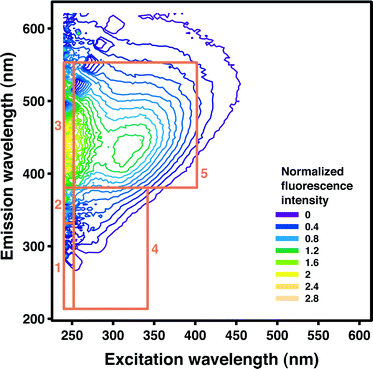
Applied to natural or treated waters, fluorescence spectroscopy is often used to measure the intensity of fluorophores associated with humic acids, fulvic acids, and proteins. Humic-like substances typically represent the majority of fluorophores in both lake and river waters.⁷ Fluorophores are frequently grouped according to their tendency to fluoresce in five distinct regions of the FEEM.⁸Table 1 lists the excitation and emission wavelength ranges used in this study to delineate these regions, and a visual representation is provided in Fig. 1. The fluorescence intensity within each region may be integrated to aid in interpretation of FEEMs and to quantify region-specific changes in fluorescence.⁸ This procedure is known as fluorescent regional integration (FRI). Although FRI is easily applied for FEEM data management, it may not capture subtle characteristics of fluorescence spectra.

Table 1 Excitation and emission wavelength ranges for fluorescent regions I–V. The proportions of total FRI signal due to each region in treated water from Pottle and Pockwock lakes are also listed

Region	Characteristics	Excitation wavelength (nm)	Emission wavelength (nm)	Pottle Lake FRI signal (%)	Pockwock Lake FRI signal (%)
a Lower limit was extended from 280 nm to 200 nm to match the detector range.
Region I	Aromatic protein I	200–250	200–330^a	1.3	1.0
Region II	Aromatic protein II	200–250	330–380	1.8	2.1
Region III	Associated with fulvic acids	200–250	380–550	14.8	15.2
Region IV	Soluble microbial products	250–340	200–380^a	8.2	9.2
Region V	Associated with humic acids	250–400	380–550	74.0	72.6

---

Fig. 1 A FEEM from the bench-scale advanced oxidation experimental data with fluorescent regions I–V superimposed.

Linear regression using FRI regions as inputs has been employed previously for the prediction of DBP formation in drinking water.⁹ Principal components¹⁰ and parallel factor analysis (PARAFAC)^10–13 have also been successful for DBP prediction using fluorescence spectra. The objective of this study was to compare two previously applied methods—FRI and principal components regression—for THM and HAA prediction via fluorescence to three approaches that have not been applied in this context: supervised principal components regression, the lasso and boosted regression tree ensembles. While principal components regression is effective for finding linear combinations of inputs (excitation–emission coordinates) that exhibit large variance within a data set, supervised principal components regression seeks linear combinations that have high variance and high correlation with the outcome—DBP formation. This is accomplished by eliminating excitation–emission pairs that are irrelevant for prediction prior to computing the principal components. Boosted regression tree ensembles and the lasso also eliminate irrelevant inputs, and in high-dimensional settings, typically yield models that depend on just a small fraction of the input variable set—a benefit for interpretation. These statistical learning methods, applied to DBP prediction, retain some of the interpretability of FRI while offering improved prediction accuracy over both FRI and principal components regression.

2. Methods

2.1. Data collection

2.1.1. Drinking water treatment plant data. Water samples were collected from the JD Kline Water Supply Plant in Halifax, Nova Scotia, Canada. A full description of this direct-filtration facility has been provided elsewhere.^14,15 Typical values for key parameters in raw and treated water are given in Table 2.¹⁶ Instantaneous HAA and THM concentrations were measured in treated water samples and ranged from 24.4–50.8 (N = 5) and 6.6–38.4 μg L⁻¹ (N = 11), respectively. HAA and THM formation potentials (HAAfp and THMfp) were measured, according to the method of Summers et al.,¹⁷ in post-filter water samples and in flocculated water samples passed through a 0.45 μm polysulfone filter. HAAfp and THMfp ranged from 23.9–60.1 (N = 17) and 19.9 to 103.3 μg L⁻¹ (N = 26), respectively. Fig. 2 provides a summary of the distribution of DBP concentrations according to formation conditions and source water.

Table 2 Typical values for raw and treated water from Pockwock and Pottle lakes

Parameter	Pockwock (raw)	Pockwock (treated)	Pottle (raw)	Pottle (treated)
Alkalinity (as CaCO3)	<1.0 mg L^−1	20.0 mg L^−1	8.2 mg L^−1	23 mg L^−1
Hardness (as CaCO3)	4.8 mg L^−1	12.0 mg L^−1	12 mg L^−1	12 mg L^−1
Total organic carbon	2.5 mg L^−1	1.5 mg L^−1	1.6 mg L^−1	1.5 mg L^−1
pH	5.7	7.3	6.95	7.14
Turbidity	0.26 NTU	0.06 NTU	0.25 NTU	<0.1 NTU
Iron	0.054 mg L^−1	<0.05 mg L^−1	<0.05 mg L^−1	<0.05 mg L^−1
UV254	0.099 cm^−1	0.041 cm^−1	n/a	0.050 cm^−1

---

Fig. 2 Box^a and whisker^b plots of THM and HAA observations on full-scale WTP (left column) and bench-scale (right column) samples. DBP formation in WTP samples is divided by formation conditions—uniform (FP) or instantaneous. ^aBoxes enclose the interquartile range (IQR) and heavy black lines represent medians. ^bWhiskers extend from the upper and lower quartile to the most extreme value within 1.5 times the IQR.

2.1.2. Bench-scale advanced oxidation data. Filtered water from the Pottle Lake Water Treatment Plant (Sydney, Nova Scotia) was used as the working matrix for the bench-scale advanced oxidation process experiments. This facility employs ultrafiltration for NOM removal, sodium hydroxide for pH control, and free chlorine for disinfection. The significant presence of hydrophilic NOM in the source water—poorly removed by the treatment process—has resulted in elevated HAA concentrations in distributed water. Typical values for key water quality parameters are provided in Table 2.¹⁸

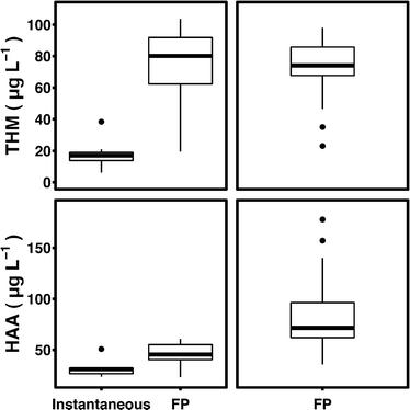
Water samples were treated with hydrogen peroxide or ozone at 1 or 10 mg L⁻¹ and exposed to UV fluences of 100 or 1000 mJ cm⁻²via a bench-scale collimated beam unit (PS1-1-120, Calgon Carbon) equipped with a 1000 W medium-pressure mercury-UV lamp. The dosing procedure for determining fluence is described in Bolton and Linden.¹⁹ Hydrogen peroxide was dosed from a 3 mg mL⁻¹ stock solution and quenched with bovine catalase (Worthington Biochemical). Ozone was applied via an ozone generator (Azcozon VMUS – 04(O2)) operated at 2 L min⁻¹ and 40 psi. Samples were collected in 40 mL glass vials and stored at 4 °C prior to analysis. DBP formation potentials for all samples were measured according to Summers et al.¹⁷ and ranged from 36.4 to 178.0 μg L⁻¹ and 23.0 to 97.7 μg L⁻¹ for HAAfp and THMfp, respectively (Fig. 2).

2.1.3. Fluorescence spectroscopy. A benchtop fluorometer (Horiba Aqualog) was used to generate all FEEMs used in predictive models—an example FEEM from the bench-scale experimental data set is provided in Fig. 1. The instrument had an excitation range of 230–610 nm and an emission range of 250–620 nm. The integration interval and spectral resolution were 0.1 seconds and 3 nm, respectively. Before acquiring data, a deionized water (Milli-Q Gradient A10) blank was used to validate the performance of the xenon lamp and to measure the signal-to-noise ratio. FEEMs were normalized and pre-processed to remove the inner filter effect and both 1st and 2nd order Raleigh scattering. Data were subsequently processed using an FRI algorithm, as described by Chen et al.⁸ The regions specified in Table 1 were used to delineate the boundaries for each of the integrations.

2.1.4. THM and HAA quantification. Quantification of THMs and HAAs was performed according to US EPA Methods 552.1 and 552.2. For THM and HAA analysis, liquid–liquid extraction by pentane and methyl tert-butyl ether (MTBE), respectively, was employed prior to detection by gas chromatography with an electron capture detector (GC-ECD). All DBP analysis was performed using a Varian CP-3800 gas chromatograph equipped with a Varian CP-8400 autosampler and an Agilent VF-5 ms column of dimensions 30 m × 0.25 mm × 0.25 μm. High purity helium was used as the carrier gas in all separations. Method detection limits for chloroacetic, bromoacetic, dichloroacetic, trichloroacetic, bromochloroacetic, dibromoacetic, tribromoacetic, bromodichloroacetic, and chlorodibromoacetic acids were 4.0, 2.5, 2.0, 1.5, 1.5, 1.0, 8.5, 2.0, and 3.2 μg L⁻¹, respectively. Method detection limits for chloroform, dichlorobromomethane, dibromochloromethane, and bromoform were 1.5 μg L⁻¹.

2.2. Statistical methods

2.2.1. Pre-processing and cross-validation. Since data collected at the full-scale treatment plant included both instantaneous DBP concentrations and formation potentials, a binary variable was used to differentiate between the two. This variable was included in the input matrix for lasso models and boosted regression tree ensembles and included in a linear model with the optimal number of principal components or the regional integrations otherwise.

A typical FEEM included excitation–emission wavelength pairs, or features, that contained little-to-no variance over a given data set. Accordingly, the 5500 features with the largest variance in fluorescence intensity were pre-selected for inclusion in all predictive models (except FRI), yielding N × 5500 input matrices with N corresponding to sample size (N = 60 for bench-scale THMfp and HAAfp, N = 22 for full-scale HAA(fp) and N = 37 for full-scale THM(fp)—full-scale water treatment plant (WTP) input matrices had 5501 features including the formation potential indicator).

Prediction error was estimated via nested k-fold cross-validation on the data, with k equal to 5 (full-scale WTP samples) or 10 (bench-scale experimental data). Nested cross-validation allows for training of each model and validation of its predictive accuracy—independent of model fitting—all on a single data set.²⁰ For each model, tuning parameters were optimized via the inner cross-validation loop (k-fold cross-validation on the k-1 training folds) and prediction error was estimated via the outer cross-validation loop. Model performance was assessed using the average of the mean absolute prediction error estimates over 10 iterations of the full nested cross-validation procedure.

2.2.2. Supervised principal components regression. Supervised principal components regression^21,22 is a modification of principal components regression that seeks components that capture variance within the data and are also correlated with the outcome. Supervised principal components regression models were trained as follows: the standardized univariate linear regression coefficients were computed for the response on each feature separately, and features with coefficients greater than a threshold θ in absolute value were retained. M principal components of the reduced input matrix were then used in a linear regression model, with θ and M chosen by cross-validation. Principal components regression models²³ on the full 5500 feature set were tuned by selecting the optimal number of components, M, using cross-validation.

2.2.3. The lasso. The lasso^24,25 is a linear regression method that incorporates a penalty into the least-squares criterion equal to the l₁ norm of the coefficient vector β. The l₁ penalty has the effect of shrinking the coefficient estimates towards zero and setting a number of them exactly to zero. This property encourages sparse solutions that depend on a subset of all possible features (predictors) and is particularly useful in prediction problems where the number of features exceeds the number of observations. Lasso models were tuned by optimizing the regularization parameter λ, a multiplier on the l₁ penalty term.

2.2.4. Boosted regression tree ensembles. Boosted regression tree ensembles^26–28 merge function approximation via regression trees with boosting, an adaptive method for combining simple models. Regression trees partition the feature space into rectangular regions and fit a constant to each—for a given region this is the mean response for the observations that region contains.²⁰ Boosting is an iterative procedure that fits regression trees sequentially, each to the residuals of the previous model. At each step, the model is updated to include the most recent tree. The algorithm proceeds in stagewise fashion—that is, trees added to the ensemble are left unchanged at subsequent iterations—and the contribution of each tree is shrunk by a learning rate that allows a greater number of trees to be included in the final model.²⁹ The resulting ensemble is a linear combination of all the fitted trees. Boosted regression tree ensembles were trained with a squared error loss function and number of boosting iterations as the sole tuning parameter. Other model parameters were selected based on heuristics given by Elith et al.²⁹ and Hastie et al.²⁰ Owing to computational considerations, features were pre-selected, as a step in the inner cross-validation loop, from the initial set by a preliminary application of the boosted tree algorithm. Those features that did not contribute to a reduction in squared error were eliminated. For the bench-scale data, at each boosting iteration a regression tree was fitted to a random sample of 50% of the data. Sub-sampling has been shown to improve prediction accuracy in boosted regression tree ensembles,²⁷ but none was carried out on full-scale WTP data sets due to the smaller number of observations.

3. Results and discussion

3.1. FRI analysis

FRI analysis of Pottle and Pockwock lake waters is summarized in Table 1. In samples from both sources, the fluorescent signal was dominated by fluorophores characteristic of humic acids (region V). Fulvic acid-associated compounds were responsible for the second greatest contribution to fluorescent NOM (region III). The minimal contribution to the FEEM profile of regions associated with biological activity is consistent with the low dissolved organic carbon content of the source waters.

3.2. Model predictions

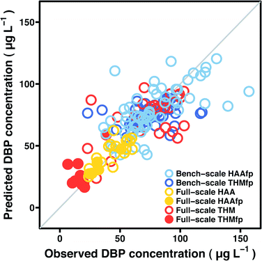
Model prediction performance is summarized in Tables 3–4 and Fig. 3. Table 3 lists mean absolute error for the five model types, applied to HAA and THM formation potentials on post-filter Pottle Lake water treated by bench-scale advanced oxidation processes. Table 4 displays the same metric for data collected at the full-scale treatment facility—error estimates in Table 4 represent prediction of both instantaneous DBP concentrations and DBP formation potentials. Fig. 3 shows cross-validation test fold predictions by the most accurate model for each data set against the corresponding observed DBP concentrations. Test fold predictions represent observations that were excluded from model fitting at a given iteration of the cross-validation procedure and may be understood as an assessment of how a given predictive model will generalize to an independent data set. Explicit model expressions are provided in Tables S1–S5 (ESI†). Since boosted tree ensembles lack a succinct expression, spectral features that contributed substantially to a reduction in squared error for each data set are listed in Tables S6–S8.†

Table 3 Mean absolute error for five model types on data generated via advanced oxidation processes at bench-scale

Bench-scale HAAfp (N = 60)	Mean absolute error (μg L^−1)
a Pre-conditioning improved mean absolute error to 10.2 μg L^−1.
Lasso	14.9
Supervised principal components	15.3
Boosted regression tree ensemble	15.7
Principal components regression	16.7
FRI linear regression	18.3

---

Bench-scale THMfp (N = 60)	Mean absolute error (μg L^−1)
Supervised principal components	9.5
Boosted regression tree ensemble	10.7
Principal components regression	11.5
FRI linear regression	11.7
Lasso	11.8^a

---

Table 4 Mean absolute error, ordered from least to greatest, for five model types on data representing full-scale WTP samples

Full-scale WTP HAA/HAAfp (N = 22)	Mean absolute error (μg L^−1)
Lasso	7.7
Boosted regression tree ensemble	7.8
Supervised principal components	7.9
FRI linear regression	9.7
Principal components regression	9.8

---

Full-scale WTP THM/THMfp (N = 37)	Mean absolute error (μg L^−1)
Boosted regression tree ensemble	13.5
Lasso	17.8
Supervised principal components	17.8
FRI linear regression	20.7
Principal components regression	21.7

---

Fig. 3 Observed DBP concentrations against cross-validation test fold predictions by the most accurate model for each data set—the y = x line is superimposed.

The prediction accuracy of FRI regression models for HAA(fp) and THM(fp) on Pottle and Pockwock lake water was not competitive with the most accurate methods. However, the accuracy of FRI regression did exceed that of principal components regression for full-scale WTP THM(fp) and HAA(fp) prediction (Table 4). Least squares linear models do have one major advantage over other model types in that they allow for statistical inference—region V, characteristic of humic acid fluorescence, was a statistically significant predictor (α = 0.05) of DBP formation in all four FRI models (WTP HAA(fp) and THM(fp), bench-scale HAAfp and THMfp).

Principal components regression was not competitive with the highest-performing methods on any of the four data sets either, while supervised principal components regression yielded predictions that were consistently more accurate. The relatively low predictive accuracy of (unsupervised) principal components regression, especially on the full-scale WTP data, may have been due in part to insufficient information in the small number of observations to efficiently estimate the high-dimensional covariance matrices of the spectral features. The large number of apparently irrelevant features may have also affected performance—the supervised principal components procedure tends to eliminate such features and derives the components from a lower-dimensional set. On average, the first 5 and 21 components, respectively, were selected via the inner cross-validation loop for bench-scale HAAfp and THMfp prediction by principal components regression. For full-scale WTP HAA and THM predictions—including formation potentials—the first 9 and 7 components, respectively, were selected on average. Cross-validation for supervised principal components regression typically selected fewer components, each a linear combination of a reduced set of spectral features. Still, this does not compare to the parsimony of the lasso, where the number of non-zero coefficients is equal to the sample size, at most.³⁰

The lasso overcomes high dimensionality by employing l₁-regularization, yielding sparse models that depend on a subset of the full feature set. However, this property did not always result in improved prediction accuracy over supervised principal components regression—the lasso showed evidence of overfitting when applied to the bench-scale THMfp data. Pre-conditioning for feature selection can retain the predictive accuracy of supervised principal components and the simplicity of the lasso in situations where the former exhibits superior prediction performance.³¹ This is done by applying the lasso to the supervised principal components regression predictions, which serve as a de-noised surrogate for the DBP outcome. Preconditioning improved the mean absolute error of lasso test-fold predictions on the bench-scale THMfp data from 11.8 to 10.2 μg L⁻¹, for example.

Hastie et al.^20,32 show that boosting can also be understood as an l₁-regularization procedure. Boosted regression tree ensembles yielded sparse models and accurate predictions, especially on the smaller full-scale data sets. Notably, boosted ensembles exhibited higher prediction accuracy on the full-scale WTP THM(fp) data than any of the alternatives. This may be explained by the non-linearity of the boosted tree function estimate and the ability of regression trees to model interactions among features.

Overall, boosted regression tree ensembles, the lasso, and supervised principal components regression were effective for DBP prediction with fluorescence spectra as inputs. Moreover, the small number of observations and non-uniformity of sample treatment presented a challenging prediction task—it is expected that larger, more uniform data sets would have yielded lower test errors.

3.3. Spectral feature selection

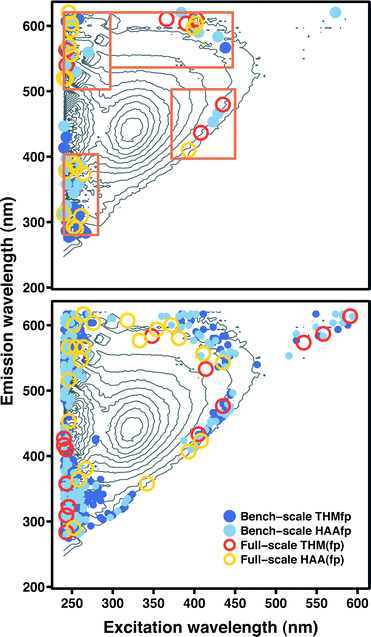
The feature selection inherent in boosted regression tree ensembles and the lasso could be advantageous in some situations because it yields more interpretable models. Essentially, these model types combine some of the simplicity of FRI with a higher degree of predictive accuracy. The top panel in Fig. 4 displays the spectral features (excitation–emission coordinates) with non-zero coefficients in lasso models fitted to the four data sets, superimposed on a representative FEEM. The bottom panel displays the spectral features that account for 95% of relative influence in boosted tree ensembles fitted to the four data sets. Here, relative influence corresponds to the normalized average reduction in squared error attributable to each spectral feature.²⁶ For the full-scale HAA(fp) and THM(fp) data sets, 95% of the relative influence was due to just 22 and 14 features, respectively (Table S6, ESI†). Influence was more widely distributed in ensembles fitted to the bench-scale HAAfp and THMfp data, with 95% due to 170 and 273 features, respectively (Tables S7 and S8, ESI†).

Fig. 4 (Top panel) Spectral features (excitation/emission coordinates) with non-zero coefficients in lasso models fitted to the four data sets (alternative FRI regions are superimposed). (Bottom panel) Spectral features accounting for 95% of relative influence in boosted regression tree ensembles fitted to the four data sets.

For both model types, the selected features exhibited a similar distribution across all four data sets. Features selected by the lasso were concentrated in FRI regions I–IV and almost entirely absent from region V (associated with humic fluorophores). This is in contrast to FRI linear regression models, where region V was a significant predictor of DBP formation without exception. Instead, a number of selected features traced the upper and lower perimeter of the principal peak associated with humic fluorophores, outside of region V. Another concentration of features occurred in the upper extreme of the emission range, at the lower end of the excitation range (above region III). Notably, the lasso fit to the full-scale THM(fp) data included only seven features. In contrast to the other lasso models, none of these seven were located in FRI regions I, II, or IV, and only one was located in region III.

Features selected by boosted tree ensembles were also concentrated in regions I–IV and mostly absent from region V. In ensembles fitted to bench-scale data, a considerable number were present in region IV (characteristic of soluble microbial products). Again, a number of selected features traced the perimeter of the principal humic peak. A substantial fraction of influential features were also associated with coordinates directly above region III, but features in the ensemble fitted to full-scale THM(fp) data were absent from this area.

Feature selection can be used to identify excitation-emission pairs or, more generally, regions of the FEEM important for DBP prediction. For example, the four regions outlined in the top panel of Fig. 4 were chosen to contain most of the spectral features selected by lasso models fitted to the four data sets. Using these four regions in FRI regression models in place of the five described in Table 1 yielded improved prediction accuracy. Mean absolute error for bench-scale HAAfp and THMfp improved from 18.3 to 16.2 μg L⁻¹ and from 11.7 to 10.5 μg L⁻¹, respectively. For the full-scale WTP data, HAA(fp) prediction error improved from 9.7 to 8.8 μg L⁻¹ and THM(fp) prediction error from 20.7 to 19.6 μg L⁻¹.

Fluorescence intensity at specific excitation–emission wavelength pairs has also been proposed as a potential online indicator of changes in dissolved organic carbon.³³ This idea could be extended to anticipate changes in DBP formation in real-time, monitoring a restricted set of wavelengths.³⁴ In contrast, the derived inputs of principal components regression are linear combinations of all of the excitation/emission wavelength pairs—principal components regression is not a feature selection method and as a result, it is somewhat less interpretable.²⁰

4. Conclusion

This study demonstrated the novel application of several statistical learning methods for prediction of HAA and THM formation following bench-scale advanced oxidation process experiments and full-scale conventional treatment. Fluorescence spectra are easily acquired, and, with effective signal processing, could be used for monitoring regulated compounds in drinking water. In general, boosted regression tree ensembles and the lasso yielded accurate predictions and sparse models that depended on a small subset of the full spectral feature set. In particular, boosted regression trees provided superior predictions of THM(fp) following full-scale conventional treatment. The feature selection property of these methods offers some of the interpretability of FRI regression, which exhibited relatively poor performance. Predictions by principal components regression were less accurate than the highest performing methods, but supervised principal components regression yielded competitive prediction accuracy.

Acknowledgements

The authors acknowledge the financial support provided through the NSERC/Halifax Water Industrial Research Chair in Water Quality & Treatment at Dalhousie University. Funding partners in the Industrial Research Chair program are NSERC, Halifax Water, LuminUltra, Cape Breton Regional Municipality Water Department, and CBCL Ltd. The authors also acknowledge the technical support of Heather Daurie and Elliott Wright, chemists at Dalhousie University's Clean Water Lab, and the employees of Halifax Water.

References

1. C. M. Villanueva, K. P. Cantor, S. Cordier, J. J. K. Jaakkola, W. D. King, C. F. Lynch, S. Porru and M. Kogevinas, Epidemiology, 2004, 15, 357–367.
2. US EPA, Water: Stage 2 DBP Rule—Basic Information, http://water.epa.gov/lawsregs/rulesregs/sdwa/stage2/basicinformation.cfm, (accessed November 2015).
3. Health Canada, Guidelines for Canadian Drinking Water Quality: Guideline Technical Document—Haloacetic Acids, http://www.hc-sc.gc.ca/ewh-semt/pubs/water-eau/haloaceti/index-eng.php, (accessed November 2015).
4. Health Canada, Guidelines for Canadian Drinking Water Quality: Guideline Technical Document—Trihalomethanes, http://www.hc-sc.gc.ca/ewh-semt/pubs/water-eau/trihalomethanes/index-eng.php, (accessed November 2015).
5. S. D. Richardson, M. J. Plewa, E. D. Wagner, R. Schoeny and D. M. DeMarini, Mutat. Res., 2007, 636, 178–242.
6. R. K. Henderson, A. Baker, K. R. Murphy, A. Hambly, R. M. Stuetz and S. J. Khan, Water Res., 2009, 43, 863–881.
7. P. G. Coble, Mar. Chem., 1996, 51, 325–346.
8. W. Chen, P. Westerhoff, J. Leenheer and K. Booksh, Environ. Sci. Technol., 2003, 37, 5701–5710.
9. D. W. Johnstone and C. M. Miller, Environ. Eng. Sci., 2009, 26, 1163–1170.
10. N. M. Peleato and R. C. Andrews, J. Environ. Sci., 2015, 27, 159–167.
11. K. M. H. Beggs, R. S. Summers and D. M. McKnight, J. Geophys. Res., 2009, 114, G04001,  DOI:10.1029/2009JG001009.
12. D. W. Johnstone, N. P. Sanchez and C. M. Miller, Environ. Eng. Sci., 2009, 26, 1551–1559.
13. B. Hua, K. Veum, J. Yang, J. Jones and B. Deng, Environ. Monit. Assess., 2010, 161, 71–81.
14. A. K. Stoddart and G. A. Gagnon, J. - Am. Water Works Assoc., 2015, 107, E638–E647.
15. Y. S. Vadasarukkai, G. A. Gagnon, D. R. Campbell and S. C. Clark, J. - Am. Water Works Assoc., 2011, 103, 66–80.
16. Halifax Water, Typical Analysis of Pockwock/Lake Major Water 2013–2014, https://www.halifax.ca/hrwc/documents/Pockwock-LakeMajor2013-2014-FINAL-KM.pdf, (accessed November 2015).
17. S. R. Summers, S. M. Hopper, H. M. Shukairy, G. Solarik and D. Owen, J. - Am. Water Works Assoc., 1996, 88, 80–93.
18. CBRM, Water Utility, 2014 Annual Report, 2015.
19. J. R. Bolton and K. G. Linden, J. Environ. Eng. Div., 2003, 129, 209–215.
20. T. Hastie, R. Tibshirani and J. Friedman, The Elements of Statistical Learning, Springer, New York, 2nd edn., 2009.
21. E. Bair and R. Tibshirani, PLoS Biol., 2004, 2, 511–522.
22. E. Bair, T. Hastie, D. Paul and R. Tibshirani, J. Am. Stat. Assoc., 2006, 101, 119–137.
23. B. Mevik, R. Wehrens and K. H. Liland, PLS: Partial Least Squares and Principal Component regression. R package version 2.4-3, http://CRAN.R-project.org/package=pls (accessed November 2015), 2013.
24. R. Tibshirani, J. R. Stat. Soc. Series B Stat. Methodol., 1996, 58, 267–288.
25. J. Friedman, T. Hastie and R. Tibshirani, J. Stat. Softw., 2010, 33, 1–22.
26. J. H. Friedman, Ann. Stat., 2001, 29, 1189–1232.
27. J. H. Friedman, Comput. Stat. Data Anal., 2002, 38, 367–378.
28. G. Ridgeway, GBM: Generalized Boosted Regression Models. R package version 2.1.1, http://CRAN.R-project.org/package=gbm, (accessed November 2015), 2015.
29. J. Elith, J. R. Leathwick and T. Hastie, J. Anim. Ecol., 2008, 77, 802–813.
30. S. Rosset and J. Zhu, Ann. Stat., 2007, 35, 1012–1030.
31. D. Paul, E. Bair, T. Hastie and R. Tibshirani, Ann. Stat., 2008, 36, 1595–1618.
32. T. Hastie, J. Taylor, R. Tibshirani and G. Walther, Electron. J. Stat., 2007, 1, 1–29.
33. Y. Shutova, A. Baker, J. Bridgeman and R. K. Henderson, Water Res., 2014, 54, 159–169.
34. R. Hao, H. Ren, J. Li, Z. Ma, H. Wan, X. Zheng and S. Cheng, Water Res., 2012, 46, 5765–5776.

---

Footnote

† Electronic supplementary information (ESI) available. See DOI: 10.1039/c5ew00285k

---