Prediction of concrete corrosion in sewers with hybrid Gaussian processes regression model

Abstract

Concrete corrosion is a major concern for sewer authorities due to the significantly shortened service life, which is governed by the corrosion rate and the corrosion initiation time. This paper proposes a hybrid Gaussian Processes Regression (GPR) model to approach the evolution of the corrosion rate and corrosion initiation time, thereby supporting the calculation of service life of sewers. A major challenge in practice is the limited availability of reliable corrosion data obtained in well-defined sewer environments. To enhance the predictability of the hybrid GPR model, an interpolation technique was implemented to extend the limited dataset. The trained model was able to estimate the corrosion initiation time and corrosion rates very close to those measured in Australian sewers.

---

1 Introduction

Sewer networks mainly composed of concrete pipelines are critical infrastructure worldwide. For instance, the total assets value of sewers is estimated to be $100 billion in Australia and one trillion dollars in America.¹ However, the corrosion of sewer infrastructure is one of the critical problems facing wastewater communities, leading to the loss of concrete mass and structural capacity, cracking of the sewer pipes and ultimately structural collapse. The rehabilitation and replacement of damaged sewers involves significantly high costs. The sewer assets are being lost at an estimated annual economic cost of around $14 billion in USA alone¹ due to corrosion. This cost is expected to increase as the aging infrastructure continues to fail.^2,3

The development of corrosion on concrete sewers mainly results from the H₂S in the sewer air.^4–6 To control the corrosion problems in concrete sewers, many technologies have been devoted to remove or reduce hydrogen sulfide. Chemicals, such as nitrate or iron salts, are dosed to reduce the formation or emission of H₂S.^7–9 Other alternatives are to construct the new sewers with corrosion-resistant pipe materials or repair corroded concrete surfaces using corrosion-resistant mortar or polymer materials. To facilitate planning sewer maintenance and rehabilitation, proper estimation of the sewer service life, is critical in prioritizing limited resources. The sewer service life (L, year) is typically determined by the corrosion initiation time (t_i, month) and the corrosion rate (r, i.e., concrete depth loss over time, mm per year).

Generally, both phenomenological and data-driven models can be used to predict the sewer service life. Phenomenological models are constructed based on the first principle models, whereas data-driven models are empirical models derived from historical data collected in the processes. Phenomenological models have received significant attentions recently. The well-known Pomeroy model was used to calculate the deterioration rate of concrete sewer pipes.¹⁰ These empirical models were widely used although it fails to take into account recent findings of the corrosion process and associated impacting factors. It is recently shown that both the corrosion initiation time and corrosion rate depend on various sewer environmental factors that include the H₂S concentration, relative humidity and temperature.^11,12 Additionally, it was recently discovered that the corrosion development can be facilitated by internal cracking which is caused by the formation of corrosion products that include iron oxides precipitating in concrete.^13–15 Also, the corrosion initiation involves a combination of physical, chemical and biological processes.¹⁶ To build a proper relationship between input variables and responses, data-driven models are another alternative. Data-driven models¹⁷ including but not limited to partial least squares (PLS),^18,19 Principle Component Regression (PCR),²⁰ nonlinear PLS,²¹ support vector regression,²² artificial neural networks^23,24 are widely studied as a predicting tool. Even if a good model can be developed successfully, its estimation performance could deteriorate with the effect of uncertainties.^25–27 To account for uncertainty in input data, probability models capable of making full use of previous knowledge are more suitable for the prediction of uncertain measurements.²⁸ Probability models can lead to a potential conclusion comparable to the models based on fuzzy logic.

Gaussian Process Regression (GPR) model is a new proposed distribution-driven methodology, which is not only able to model dynamic processes of both linear and nonlinear systems, but also to generate predicted distribution (interval prediction) rather than point prediction, to facilitate our decision making for service life prediction.²⁹ Traditional models give a bare prediction without any associated confidence values and hence have to rely on the previous experience or relatively loose theoretical upper bounds on the probability of error to gauge the quality of the given prediction. On the contrary, the GPR model would become more flexible by associating confidence intervals to the predicted values. Also, through the choice of the covariance function, a wide range of modeling assumptions would be expressed to delineate unexplainable environmental factors of concrete corrosion.

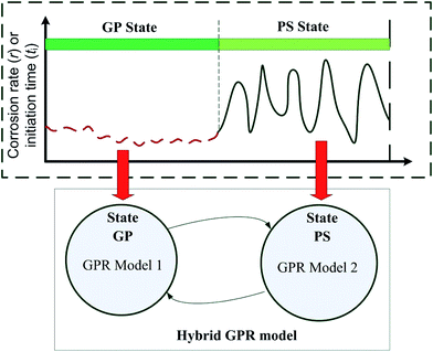
A recent long-term project reported corrosion data over 4.5 years in laboratory corrosion chambers with well-controlled conditions simulating real sewers.^8,9 They are so far the most comprehensive corrosion data covering both corrosion rate and corrosion initiation time obtained under a full range of environmental conditions, including H₂S concentration, temperature and relative humidity. This paper developed the models based on these data. These corrosion chamber studies investigated the effect of locations within the sewer on corrosion, by exposing concrete to the sewer atmosphere (simulating the pipe crown) or partially-submerging in sewage (simulating the sewer tidal region at the sewage/air interface). Since the corrosion of gas-phase (GP) and partially-submerged (PS) parts exhibited significantly different corrosion features, this study constructed separate GPR models for the two corrosion hot-spots. Furthermore, hybrid automata were proposed to coordinate the predicted results of two GPR models and formed the hybrid GPR model. The discrete changes (GP or PS) were modelled using a form of transition diagram dialect similar to state charts, while the continuous changes were modelled using the GPR model.

For the concrete corrosion, one hindering factor for the GPR model is the limited availability of historical data and incompleteness of dataset. In this paper, we interpolated the missing positions in data by the estimated samples with similar characteristics from the observed historical data, thus allowing more information to improve model prediction accuracy. Consequently, we utilized this extensive dataset to build a hybrid GPR model to predict corrosion initiation time (t_i) and corrosion rate (r), which can be used to estimate the service life for a specific sewer condition. Due to involving GPR as predicted models, both of nonlinear relationship among variables and uncertainty resulting from unexplainable factors can be approached properly. The performance and application of the proposed GPR model was further evaluated by comparison with a classical regression model, a neural network model and with observations in real sewers across Australia.

2 Material and methods

2.1 Corrosion tests in the laboratory chambers

As described in previous publications,^8,9 fresh and corroded concrete coupons were prepared separately by using a new sewer pipe (1.2 m diameter, 2.4 m length and 0.7 m thickness) from a sewer pipe manufacture (HUMES, Sydney), and a corroded concrete sewer from Sydney Water Corporation. All coupons dimensions were approximately 100 mm (length) × 70 mm (width) × 70 mm (thickness). To simulate the sewer pipe crown which is highly susceptible to sulfide induced corrosion,^27,28 the gas-phase (GP) concrete coupons were prepared. The GP coupons were embedded as pairs (1 fresh + 1 corroded) in stainless steel frames casting using epoxy (FGI R180 epoxy & H180 hardener).^11–13 The upper rim of the stainless steel frame providing a reference point for determining the change in thickness due to corrosion. One of the original surfaces of coupons, i.e. the internal pipe surface, was exposed to H₂S directly with the exposed surface facing downwards about 100 mm above the sewage (Fig. 1). Additionally, the same number of bare coupons, also prepared in pairs (1 fresh + 1 corroded), were partially submerged in the domestic sewage (PS coupons) to simulate the sewer pipe near the water level, another location which is reported to be highly susceptible to sulfide induced corrosion. For each chamber, eight pairs of enclosed coupons were exposed to the gas phase, and another eight pairs of bare coupons were partially submerged.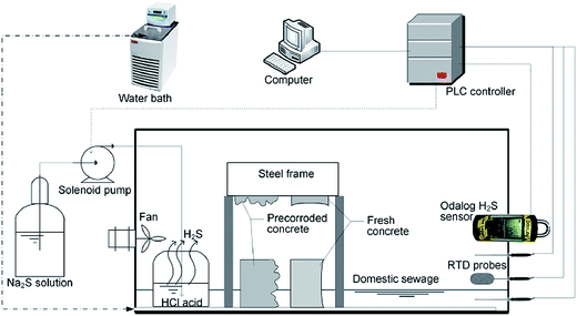

Fig. 1 Side-view of a corrosion chamber with the H₂S concentration, relative humidity, and gas temperature controlled by a program logic controller (PLC).

Thirty-six parallel corrosion chambers were established to simulate the real sewer environment controlled by a combinations of different factors, including three gas-phase temperatures (17 °C, 25 °C and 30 °C), two levels of relative humidity (RH) (100% and 90%) and six H₂S levels (0 ppm, 5 ppm, 10 ppm, 15 ppm, 25 ppm and 50 ppm). These factors were chosen based on extensive literature review of concrete corrosion processes in sewers.³⁰ Each chamber, 550 mm (L) × 450 mm (D) × 250 mm (H) in dimensions, contained 2.5 L of domestic sewage collected from a local sewer pumping station and replaced every two weeks. Other detailed constructions and installation of corrosion chambers were described previously.^8,9

During the period of chamber operation for up to 4.5 years since 2009, one set of coupons (one pair of gas-phase and one pair of partially-submerged coupons) were periodically retrieved at intervals between 6 and 10 months. A standard step-by-step procedure of sampling and analysis was employed to measure surface pH, followed by sampling for sulfur species and then photogrammetry analysis (thickness change), which has been described in previous studies.^8,9 Accordingly, the time to reach a detectable level of sulfate on the fresh concrete surface was regarded as the corrosion initiation time, t_i. According to the previous experiments, the critical levels of sulfate were arbitrarily determined as 1 g S m⁻² and 10 g S m⁻² for the gas-phase and partially-submerged concrete coupons respectively, when the location of coupons and their actual sulfide oxidation rates were taken into consideration.¹² The corrosion rate was calculated by mass loss data of corroded coupons as the thickness change per year (mm per year).

2.2 Corrosion tests in real sewers

Concrete corrosion was studied in real sewer systems to quantify corrosion occurring in working Australian sewers under a range of environmental and operating conditions. Six sewer sites were chosen in three cities, i.e. Sydney, Melbourne and Perth in Australia. The choice of three cities and two sites in each city enabled the study of different temperatures and different H₂S levels. Concrete coupons were fixed into the sewers as described³¹ and then recovered approximately every 6 months in the early stages of the project and yearly in the later stages. The retrieved coupons were analyzed similarly to the laboratory coupons for measurement of surface pH, sulfur compounds in the corrosion layer and the mass loss (thickness change)^8,9 due to corrosion. Details of the study were reported by Wells and Melchers³¹ and the corrosion initiation time and corrosion rate determined in real sewers were used to validate the proposed model in this study.

2.3 Pre-treatment of corrosion data by interpolation

The regression methods described in the previous section require the estimation of the regression coefficients. To determine these estimates, a proper amount of historical data are required. Therefore, it is necessary to extend the given data set to involve more data patterns for model training. In the lab data set, three gas-phase temperatures (17 °C, 25 °C and 30 °C) and six H₂S levels (0 ppm, 5 ppm, 10 ppm, 15 ppm, 25 ppm and 50 ppm) are collected discontinuously, which might compromise the model training and further prediction if using such few data sets. To deal with these problems, input–output relationships among existing data set were determined and the regression results were used to generate interpolation values in the intervals. This was implemented through the function ‘interpl’ in the MATLAB. Firstly, the gas-phase temperatures were interpolated into fourteen levels (17, 18, 19,…, 30 °C) for each of the six original H₂S levels by assuming that the variations of corrosion rate and time follow ‘spline’ function. Secondly, H₂S levels were generalized into ten levels (0, 5, 10,…, 50 ppm) for each of the fourteen temperature levels by assuming that variations of corrosion rate and time follow ‘cubic’ function. The interpolation function (‘interpl’, ‘spline’ and ‘cubic’) was chosen based on how well the function shape fits the corrosion data.

2.4 Hybrid Gaussian processes regression modeling

2.4.1 GPR model. GPR model is a simple and general class of functions, describing precisely any distribution over functions such that any finite set of function values {f(x₁), f(x₂),…, f(x_n)} have a joint Gaussian distribution. Given a new testing input x* with a given training set D = {(x_i, y_i)|_i=1ⁿ} of n pairs of inputs x_i and noisy outputs y_i, GPR is usually formulated to compute the predictive distribution (distribution of possible unobserved values conditional on the incoming observed values) of f. Assuming that the noise is additive, independent and Gaussian, the relationship between the function f(x_i) and the observed noisy targets y are derived by:³²

y_i = f(x_i) + ε_i (1)

ε ∼ N(0,σ_n²) (2)

f(·) ∼ GP(0,k(·,·)) (3)

where GP(0,k(·,·)) represents a Gaussian process with mean and covariance matrix equaling to 0 and k(·,·), respectively. The noise ε follows the Gaussian distribution with mean 0 and covariance σ_n². Covariance matrix is simplified as K = k_ij. By inference, it is easy to obtain that the outputs follow multivariate joint Gaussian distribution:

y ∼ N(0,K_y) (4)

where K_y = K + σ_n²I, K_y is the covariance matrix with the dimension of n × n. The corresponding (i, j)^th element is

(K_y)_ij = cov(y_i,y_j) = k(x_i,x_j) + σ_n²δ_ij (5)

where δ_ij is the Kronecker function.³³ The major difference of K and K_y is that K is noise free but K_y is noise-induced covariance matrix. In the GPR model, the most commonly used covariance matrix is Squared-Exp (SE) shown as follows:where σ_f² and l are hyper-parameters in need of identification. It should be noted that commonly-used kernels such as the Squared-Exp (SE), Neural Network (NN) or Matérn kernels are local kernels,³² depending only on the scaled Euclidean distance between two points. Therefore, models based on local kernels are particularly susceptible to the “curse of dimensionality” (the predictive power reduces as the data dimensionality increases),³⁴ and are unable to extrapolate away from the training data. Methods based solely on local kernels sometimes require exponential training examples which means many combinations of inputs. In contrast, additive kernels can allow extrapolation away from the training data. More details about kernel selection can be seen in the ESI.†

In summary, the parameters needed to be identified for aforementioned GPR model are formulated as θ = (σ_f², l, σ_n²), where l is the width of kernel k(x_i,x_j). The optimal θ can be achieved by optimize its corresponding likelihood function. The corresponding likelihood function is:

which can be optimized to derive θ. More details about the optimization can be seen in the ESI.†

The final procedure is to use the derived θ to facilitate further prediction. Since (y₁, y₂,…,y_n, f(x*))^T also following a Gaussian distribution, the prediction at the location x* can be obtained with the mean and variance:

E(f(x*)|D) = k*K_y⁻¹y (8)

var(f(x*)|D) = k(x*,x*) − k*K_y⁻¹k* (9)

where k* = (k(x*,x₁), …, k(x*,x_n))^T represents the correlated relationship between x* and training set data x_i. As shown in eqn (8) and (9), the evolution of the corrosion initiation time, t_i and the corrosion rate, r, can be monitored properly in real time by calculating E(f(x*)|D) and var(f(x*)|D). var(f(x*)|D) can be further used to represent the uncertainty level of predicted results.

2.4.2 Hybrid GPR model construction by automata. Given the hybrid features of the corrosion processes on GP and PS sewers in this paper, a tool to describe such hybrid behaviors is necessary. A hybrid automaton provides an alternative to deal with this issue. The automaton is a formal model for a dynamic system with discrete and continuous components. The semantics of a hybrid automaton is defined in terms of a labeled transition system between states, where a state consists of the current location of the automaton and the current valuation of the real variables. To formalize the semantics of the hybrid automaton, the concept of a hybrid automaton's state is firstly defined. Then, upon the constraint for each state, current valuation of the real variables can be obtained by a specified function or model. In fact, a hybrid automaton evolves depending on two kinds of transitions: continuous transitions, capturing the continuous evolution of states, and discrete transitions, capturing the changes of locations.^35,36

By using hybrid automata, the transition behaviors of GP and PS can be accounted for properly as shown in Fig. 2. More details for hybrid automata definition can be seen in the ESI.†

Fig. 2 Schematic of the hybrid GPR model.

3 Results and discussion

Prediction performance was assessed by comparing the hybrid GPR model with two scenarios, i.e. Radial Basis Function neural network (RBF) and Multivariate Linear Regression (MLR), using the original and extended data set. More details about the RBF and MLR models can be found in ESI.† All the training, testing and validation set are tabulated as the following Table 1.

Table 1 Number of data set for the training, testing and validation of models using the original or extended corrosion data

Predicted variables	Data type	Training set	Testing set	Laboratory data validation	Field data validation
Corrosion initiation time-ti (months)	Original data	20	10	10	4
	Extended data	200	80	10	4
Corrosion rate-r (mm per y)	Original data	26	10	10	17
	Extended data	208	100	10	17

---

To better define the comparative study, the models with extended data for training are defined as MLR-ex, RBF-ex and GPR-ex. On the contrary, the models with original data are formulated as MLR-or, RBF-or and GPR-or.

The number of input for all models is set to 3. A linear × SE × per kernel is used for GPR model due to the shape similarity of SVI. The Root Mean Square Error (RMSE) and correlation coefficient (r_c) were used to assess the prediction performance of inferential model. The RMSE is defined as follows for quality comparisons of different models:

where y_i and ŷ_i are the measured and prediction values, respectively.

3.1 Prediction of the corrosion initiation time (t_i)

MLR models were firstly trained and used to generate predictions of corrosion initiation time for both the GP and PS sewers, respectively. These models assumed that the corrosion initiation time is linearly dependent on the explanatory variables (variables that might affect the response variables corrosion initiation time or corrosion rate), i.e. the location of concrete, H₂S concentration (ppm), RH (%) and temperature (T). Fig. 3 suggests that, during the extended data testing period, MLR models are not able to capture the nonlinear relationship between the explanatory variables and independent variables. However, due to the interpolation, MLR-ex performed better than MLR-or slightly for both gas-phase (a) and partially-submerged (a) in the Fig. 3, which can be further confirmed in terms of RMSE and r_c in Fig. 4. The poor performance of MLR also implies that the relationship between the predictors and corrosion initiation time (t) for both of GP and PS is unlikely to be linear.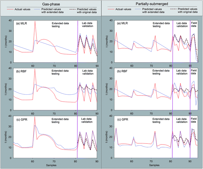

Fig. 3 Prediction of corrosion initiation time of lab and actual data of concrete corrosion using MLR, RBF and GPR for both GP (left) and PS (right) sewers.

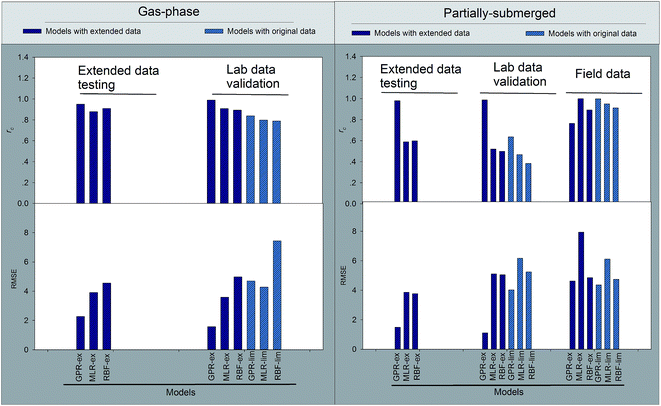Fig. 4 Comparison of RMSE and r_c under lab and actual data testing using MLR, RBF and GPR for both GP (left) and PS (right) sewers.

Secondly, RBFs are trained for GP and PS processes using the same data sets, respectively. The final structure of the RBF models for GP and PS using extended data have 23 and 21 neurons in the hidden layers. On the contrary, relative fewer neurons are obtained for the RBF models for GP (10 neurons) and PS (8 neurons) with original data. For all the scenarios, the activation functions are set to radial basis function. Even though RBF has the ability to approach nonlinear relationship between the explanatory variables and independent variables, requirement of large number of training data always make it inadequate, thus leading to even worse performance in terms of RMSE and r_c (Fig. 4).

Following the MLR and RBF models, GPR models are used to analyze the same data set. The addictive Squared-Exp (SE) covariance function is selected for all GPR models. Even though, different GPR models are generated for GP and PS processes, all parameters can be identified automatically without resorting to trial and errors necessarily. Of all three models, GPR achieved the best performance for extended data testing and laboratory data validation.

After developing the hybrid GPR model to predict t_i based upon the laboratory data, a further step was carried out to validate its performance using field data. The corrosion initiation time t_i measured for all the field sites, including two Perth sewers and two Melbourne sewers, varied from site to site but were in the range of 9 to 24 months. Also, we compared the predictions of t_i for the field sites among the MLR model, the RBF model and the GPR model. By comparing the fit between the predicted t_i and measured t_i for the four field sites it is clear that the GPR-or model achieved better accuracy for the prediction of t_i than other models with the original data for prediction. It deserved to notice that the models with extended data indeed performed better than counterpart with original data in the lab data validation, but a little bit worse during the field data validation. This is mainly due to the fact that some conditions at the field sites were far beyond the ranges for those in the laboratory corrosion chambers.³⁰

In particular, the Perth sewer site had very high H₂S concentrations, up to 830 ppm in the gas phase, and high temperatures (up to 36.6 °C), and in that situation the MLR model predicted a negative t_i. In terms of calculating the sewer service life, t_i normally contribute little to the service lifespan of a sewer pipe which is designed to last 50–100 years. However, the prediction of t_i is important to evaluate and optimize the effectiveness of a prevention strategy, such as sewer gas ventilation and chemical dosing in sewage, which is employed to prevent the initiation of corrosion. It is also important to predict the initiation of corrosion based on the operation of new sewer systems.

3.2 Prediction of the corrosion rate (r)

The linear equation for corrosion rate generated by MLR was determined. Fig. 5 suggests that, during the extended data testing period, MLR models are not able to capture the nonlinear relationship between the explanatory variables and independent variables similar to corrosion initiation time prediction. However, due to the interpolation, MLR-ex performed better than MLR-or slightly for both gas-phase and partially-submerged sewers as shown in Fig. 5a, which can be further confirmed in terms of RMSE and r_c in Fig. 6. The poor performance of MLR also implies that the relationship between the predictors and corrosion rate (r) for both of GP and PS is unlikely to be linear.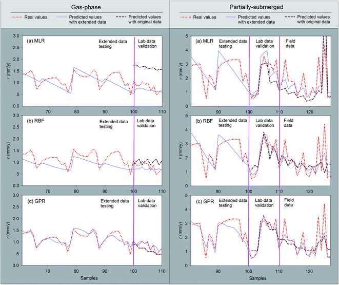

Fig. 5 Prediction of corrosion rate for laboratory and field data using MLR, RBF and GPR for both GP (left) and PS (right) sewers.

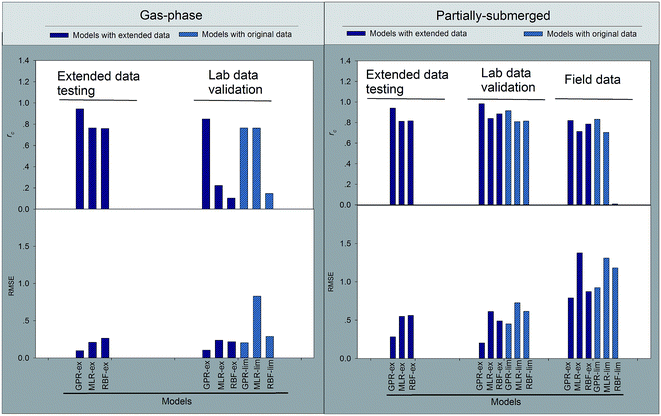Fig. 6 Comparison of RMSE and r_c obtained with laboratory and field data testing using ANN, MLR and GPR models.

To improve the prediction of corrosion rate (r), a RBF model was developed in a similar approach used for the prediction of corrosion initiation. The best architecture determined by exhaustive searching based on minimum error criterion (4-22-1 for RBF-ex under GP, 4-21-1 for RBF-ex under PS, 4-8-1 for RBF-or under GP and 4-8-1 for RBF-or under PS). The model was trained using the extended and original data sets of corrosion data obtained in the laboratory corrosion chambers and its corresponding interpolating data. The RBF model showed unacceptable performance in the extended data validation as well as lab data validation for the GP processes. On the contrary, the predictions under PS are relatively better than counterpart of GP in terms of RMSE and r_c (Fig. 6). The RBF model demonstrated improved predictions of corrosion rates by interpolating proper data points in the lab data, while under-predicting the corrosion rates for the models with original data (Fig. 5).

Finally, the GPR models were evaluated to predict corrosion rate based upon the original laboratory data and its corresponding extended data. Modeling procedures are performed as RBF model. For all the scenarios, the GPR-ex and GPR-or for both GP and PS sewers achieved the best performance with RMSE being lower than 0.2 and r_c being higher than 0.8 (Fig. 6).

By comparing the fit between the predicted and measured corrosion rate for the seventeen field sites it is clear that the GPR-or model achieved relatively better accuracy for the prediction of corrosion rate than other models with original data for prediction. It deserved to notice that the models with extended data indeed performed better than counterpart with original data for both of the lab data and field data validation. The prediction capacity of corrosion rate can be used to evaluate and optimize those corrosion prevention strategies.

3.3 Model uncertainty analysis

Even though H₂S, RH and location are taken into account by the proposed GPR models and make it adequate for corrosion rate and corrosion initiation time prediction, there are still considerable unexplained variables in the GPR predictions, such as the ignorance of other influential variables and inherent scattering in the data.

Such ignorance will further result in uncertainties to frustrate decision-making. Different from RBF and MLR models using point prediction without taking into account uncertainties, GPR is able to generate variance to envelope uncertainties properly. Such envelopes represent different levels of confidence on the prediction results. It is obvious in Fig. 7 that the boundaries of GPR models for GPR-or are capable of enveloping most of the variations of real values approximately. Even though some predicted values crossed over the 90% confident limit, the predicted results for both of GPR-ex models (GP and PS sewers) are acceptable. To qualify how reliable obtained predictive regions are, we count the percentage of wrong predictive intervals (out of envelop); in other words, how many times the GPR model fails to give a predictive region that contains the real output of every test sample. The results in Table S1 in the ESI† show that the validity of GPR models is under 90%: the rate of successful predictions is at least equal to the desired accuracy. Fig. 7 complements part of the information given in Table S1† for predicting with 90% confidence. It shows that the prediction uncertainty is an important issue for a model with new data updating. During the transition stage, some of the input variables are adjusted to bring the process to a new steady state. The confidence would be widened due to the adjusted process variables derivative from steady state values.

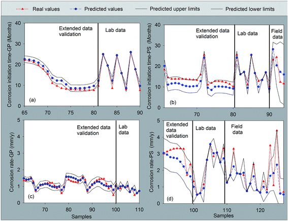Fig. 7 Uncertainty analysis of GPR models based on laboratory and field corrosion data for both of GP and PS sewers.

4 Discussion

The present work investigated the use of GPR models for the prediction of corrosion initiation time and corrosion rate in sewer networks. Hybrid automata approach provides a simple, but powerful tool to coordinate different GPR models to approach different processes of GP and PS sewers, respectively. This, along with confident levels that were generated from GPR models, supported a better prediction capacity of the concrete service life. This is to our knowledge the first time that hybrid GPR models has been achieved for concrete corrosion management.

Different from traditional black-box model-based prediction, GPR model is able to generate the confident levels to describe the uncertainty from the model parameters as well as external unexplained factors. Also, due to the limited availability of historical data, traditional black-box models are not capable of capturing the nonlinear actual variations of concrete corrosion. Thus, it is imperative to analyze the derived data and extract more features to facilitate model building. By the deep investigation of derived data, the temperature and H₂S data are interpolated properly to make sure a sufficient amount of historical data available for model building. On the contrary, due to too few data for RH, RH interpolation could result in deviation of original data and is therefore not considered in this paper.

Although most of the data used for modelling came from the lab experiments instead of real sewer networks, the results are still convincing and suitable for the model building, since the experiments were long-term (4.5 years) conducted in purpose-built corrosion chambers that has well-controlled conditions. Indeed, the controlled factors i.e. H₂S gas-phase concentration, RH and temperature are demonstrated to significantly affect the corrosion processes thus they are indispensable for corrosion modelling. However, the corrosion data obtained in real sewers might be subjected to more complicated situations. Likely, the H₂S concentration shows high variation due to the sewage flow dynamics and fluctuations of other environmental factors. Similarly, other critical but non-defined variables may still exist but have not been considered due to the confined corrosion knowledge. In order to achieve efficient modelling of concrete corrosion, further research is needed to determine the specific effects of those unexplained factors on the corrosion of concrete sewers.

In this study, we demonstrated the advantage of a new modelling approach in the prediction of sewer service life for better sewer corrosion management. While we used an advanced model giving realistic representations of corrosion, the model requires further verification through application to different sewer networks. Furthermore, although the corrosion of GP and PS sewers are divided and modeled separately, some GP sewer might be also subjected to short term submersion (similar to PS conditions). The prediction performance in such circumstances require further investigation and improvement through field studies, although the model has previously been demonstrated efficient to predict corrosion initiation time and corrosion rate properly in some sewers. This will be an important and interesting research question for future research.

5 Conclusions

This study developed a predicting tool for the estimation of the service life of concrete sewers based on the modeling of sewer corrosion through a hybrid Gaussian processes regression model. The GPR model was trained and validated with long-term (4.5 years) corrosion data obtained in laboratory corrosion chambers and corresponding interpolated data set, further verified with field measurements in real sewers across Australia. Hybrid Gaussian processes regression model achieved the best performance for both of extended and limited data in terms of RMSE and correlation coefficient compared with MLR and RBF. The derived variances of hybrid Gaussian processes regression model are able to envelope the prediction uncertainties efficiently, thus supporting better decision making of rehabilitation and replacement of damaged sewers. Hybrid GPR model can be used to predict the evolution of the sewer corrosion and be further improved by including more affecting factors or training with corrosion data under broader conditions including H₂S concentration, humidity and temperature.

Acknowledgements

This work was supported by the National Natural Science Foundation of China (61403142, 61673181), the National Natural Science Foundation of Guangdong Province, China (2015A030313225), the Science and Technology Planning Project of Guangdong Province, China (2016A020221007). Yarong Song acknowledges the support of CSC scholarship. Dr Guangming Jiang is the recipient of a Queensland State Government's Early Career Accelerate Fellowship and an Australian Research Council DECRA Fellowship (DE170100694).

References

1. M. P. H. Brongers, P. Y. Virmani and J. H. Payer, Drinking Water and Sewer Systems in Corrosion Costs and Preventative Strategies in the United States, 2002.
2. U. EPA, Hydrogen sulphide corrosion in wastewater collection and treatment system, 1991.
3. R. Sydney, E. Esfandi and S. Surapaneni, Water Environ. Res., 1996, 68, 338–347.
4. T. Hvitved-Jacobsen, J. Vollertsen and A. H. Nielsen, Sewer Processes: Microbial and Chemical Process Engineering of Sewer Networks, CRC Press, 2nd edn, 2013.
5. G. Jiang, J. Sun, K. R. Sharma and Z. Yuan, Curr. Opin. Biotechnol., 2015, 33, 192–197.
6. G. Jiang, M. Zhou, T. H. Chiu, X. Sun, J. Keller and P. L. Bond, Environ. Sci. Technol., 2016, 50, 8084–8092.
7. Y. Liu, R. Ganigué, K. Sharma and Z. Yuan, Water Sci. Technol., 2013, 68, 2584–2590.
8. Y. Liu, R. Ganigué, K. Sharma and Z. Yuan, Water Res., 2016, 98, 376–383.
9. J. Sun, X. Dai, Y. Liu, L. Peng and B.-J. Ni, Chem. Eng. J., 2017, 309, 454–462.
10. R. D. Pomeroy and A. G. Boon, The Problem of Hydrogen Sulphide in Sewers, Clay Pipe Development Association, London, 2nd edn, 1990.
11. G. Jiang, J. Keller and P. L. Bond, Water Res., 2014, 65, 157–169.
12. G. Jiang, X. Sun, J. Keller and P. L. Bond, Water Res., 2015, 80, 30–40.
13. G. Jiang, E. Wightman, B. C. Donose, Z. Yuan, P. L. Bond and J. Keller, Water Res., 2014, 49, 166–174.
14. J. Monteny, E. Vincke, A. Beeldens, N. De Belie, L. Taerwe, D. Van Gemert and W. Verstraete, Cem. Concr. Res., 2000, 30, 623–634.
15. A. K. Parande, P. L. Ramsamy, S. Ethirajan, C. R. K. Rao and N. Palanisamy, Proc. Inst. Civ. Eng. Munic. Eng., 2006, 159, 11–20.
16. A. P. Joseph, J. Keller, H. Bustamante and P. L. Bond, Water Res., 2012, 46, 4235–4245.
17. R. Nasir, H. Mukhtar and Z. Man, RSC Adv., 2016, 6, 30130–30138.
18. S. Wold, M. Sjöström and L. Eriksson, Chemom. Intell. Lab. Syst., 2001, 58, 109–130.
19. W. Shao, X. Tian, P. Wang, X. Deng and S. Chen, Chemom. Intell. Lab. Syst., 2015, 144, 108–121.
20. Y. Liu, Y. Pan, Z. Sun and D. Huang, Ind. Eng. Chem. Res., 2014, 53, 3272–3282.
21. C. Durante, M. Cocchi, M. Grandi, A. Marchetti and R. Bro, Chemom. Intell. Lab. Syst., 2006, 83, 54–65.
22. W. Yan, H. Shao and X. Wang, Comput. Chem. Eng., 2004, 28, 1489–1498.
23. G. Jiang, J. Keller, P. L. Bond and Z. Yuan, Water Res., 2016, 92, 52–60.
24. P. Kaur, V. K. Sangal and J. P. Kushwaha, RSC Adv., 2015, 5, 34663–34671.
25. F. Ahmed, S. Nazir and Y. K. Yeo, Korean J. Chem. Eng., 2009, 26, 14–20.
26. J. Ciba, P. Dydo, J. Kluczka and A. Smolin, Chemosphere, 2009, 76, 565–571.
27. P. Facco, F. Doplicher, F. Bezzo and M. Barolo, J. Process Control, 2009, 19, 520–529.
28. R. Willink, Measurement Uncertainty and Probability, Cambridge University Press, 2013.
29. W. Ni, K. Wang, T. Chen, W. J. Ng and S. K. Tan, Contr. Eng. Pract., 2012, 20, 1281–1292.
30. R. E. M. T. Wells and P. Bond, Proceedings of Corrosion and Prevention 2009, Australasian Corrosion Association, Coffs Harbour, 2009.
31. T. Wells and R. E. Melchers, Cem. Concr. Res., 2014, 61–62, 1–10.
32. C. E. Rasmussen and C. K. I. Williams, Gaussian Processes for Machine Learning, MIT Press, London, 2006.
33. K. Chalupka, C. K. I. Williams and I. Murray, J. Mach. Learn. Res., 2013, 14, 333–350.
34. Y. Bengio, Foundations and Trends® in Machine Learning, 2009, vol. 2, pp. 1–127.
35. M. Uzam and G. Gelen, Contr. Eng. Pract., 2009, 17, 1174–1189.
36. S. Paoletti, A. L. Juloski, G. Ferrari-Trecate and R. Vidal, Eur. J. Contr., 2007, 13, 242–260.

---

Footnote

† Electronic supplementary information (ESI) available. See DOI: 10.1039/c7ra03959j

---