 Open Access Article
Creative Commons Attribution 3.0 Unported Licence
Random forest and multilayer perceptron for predicting the dielectric loss of polyimide nanocomposite films
H. Guo *a,
J. Y. Zhaoab and
J. H. Yinc
aCollege of Computer Science and Engineering, Dalian Nationalities University, 18 Liaohe West Road, Dalian Development Zone, Dalian 116600, China. E-mail: guohai@dlnu.edu.cn
bFaculty of Electronic Information and Electrical Engineering, Dalian University of Technology, Dalian 116023, China
cSchool of Applied Science, Harbin University of Science and Technology, Harbin 150080, China
First published on 15th June 2017
Abstract
As a new insulating material, nanoscale thin dielectric films have been widely used in variable frequency motors, electron devices and other fields. Dielectric loss is a key performance parameter of this material. Currently, studies on the dielectric properties of polymer matrix nanocomposite films are based mostly on experiments that are costly and time-consuming. In this article, an integrated method that combines experiment and ensemble learning is applied. In situ polymerization is employed to prepare 32 polyimide matrix nanocomposite films that have different weight ratios, sizes and thicknesses and that are doped with different inorganic nanoscale particles. The dielectric losses of these 32 prepared films are measured as well. Ten multilayer perceptrons are integrated into a random forest and multilayer perceptron (RF-MLP) model using the random forest (RF) method. As shown in the experimental results, under the 10-fold cross validation, the correlation coefficient, the mean absolute error, the root mean squared error and the root relative squared error of the RF-MLP model are 0.9447, 0.0007, 0.0013 and 32.0972%, respectively. The deviation between the predicted value and the measured value is small. The RF-MLP model has a better prediction performance than other single models, such as linear regression, backpropagation neural network, radial basis function neural network, support vector regression and multilayer perceptron as well as other ensemble learning methods, such as bagging, boosting and RF-decision stump. Therefore, the RF-MLP model is a fast and reliable method applicable to predicting the properties of the new nano-dielectric material and other materials.
Introduction
Polyimide is a polymer of the imide monomer unit (–CO–N–CO–), as a part of the main chain. Among the polyimides, phthalimide is the most important structure. As a specially engineered material, polyimide has been commonly used in many fields, including aerospace, aviation, variable frequency motors, microelectronics, nanometre, liquid crystals, separating membranes, lasers and so on. Polyimide has now been globally researched, developed and utilized and is listed as one of the most promising engineering plastics in the 21st century.1,2 In recent years, polyimide matrix nanocomposite films have attracted a great deal of academic attention. By doping different inorganic nanoparticles into the polyimide, many researchers and scholars have acquired better electrical, thermal and mechanical properties of the material.3–8 As a key electric property of nanocomposite film, dielectric loss can be affected by a number of factors, such as the type, the dielectric constant, the electrical resistivity, the thermal conductivity, the size and the specific surface area of the doped nanoparticle as well as by the doping ratio and the film thickness.9–12 In 1997, the E. I. Du Pont Company, ABB and Siemens spent a great deal of effort and time on testing over 4000 materials and finally synthesized the CR-corona resistant polyimide films, such as Kapton-CR and Kapton-FCR, which have been widely used in European high-speed electric locomotives. Their corona resistance is 500 times as high as that of a conventional polyimide films. It is for this reason that developing a fast and efficient method to predict the dielectric loss of polyimide nanocomposite films is urgent and important.ANNs (artificial neural networks) has been extensively applied for predicting film properties. Bahramian Alireza et al. simulated and predicted the growth rate of TiO2 nanostructured thin films by using a feed-forward back-propagation network.13 Ko Young-Don et al. made use of PCA (principle component analysis)-based neural networks to predict the physical and material properties of an HfO2 thin film.14 Nobrega Marcelo Medre et al. predicted the mechanical and barrier properties of biodegradable films by using the SOMs (self-organizing maps) neural network. The deviation between the predicted value and the measured value was not higher than 24%.15 M. Payandehdoost et al. optimized the group method of data handling (GMDH)-type neural networks by means of genetic algorithms to predict present separate polynomial relations for the area-weighted average film cooling heat transfer coefficient.16 Also using a neural network, Piliougine Michel et al. characterized the electrical parameters of several thin-film photovoltaic module technologies.17 Yang Yu-Sen applied a generalized regression neural network (GRNN) for predicting the friction coefficient of deposited Cr1−xAlxC films on high-speed steel substrates via direct current magnetron sputtering systems.18 By taking advantage of the neural network, these researchers did well in predicting film properties. However, there are still problems: (1) only conventional films are used for the predictions, and no studies on predicting properties of new nanocomposite films have been reported; (2) only single films are used for regression prediction, and very few studies have been conducted on predicting the properties of films doped with different particles, and; (3) the accuracy of the single neural network prediction model needs to be further improved.
Polymeric nanocomposites are a new type of dielectric. However, there is no report on using intelligent computing together with neural networks technology to predict its dielectric loss. On an experimental basis, this paper makes use of a RF-optimized MLP ensemble learning model to predict the dielectric loss of the polyimide nanocomposite films. In the following, materials and experimental procedures are introduced first. The construction of the sample library and the prediction model are described next. Then, experimental results are described and the establishment of the RF-MLP model with 10-fold cross validation results is carried out. The 10-fold cross validation are also progressed for discussing the accuracy of the RF-MLP model and the single prediction models, including BP (back-propagation) neural network, RBF (radical basis function) neural network, SMO-SVR (sequential minimal optimization-support vector machine), MLP (multilayer perceptron) neural network and linear regression. Comparisons to other ensemble learning methods are also made. Finally, the paper concludes with a summary of this study.
Experimental
Film preparation
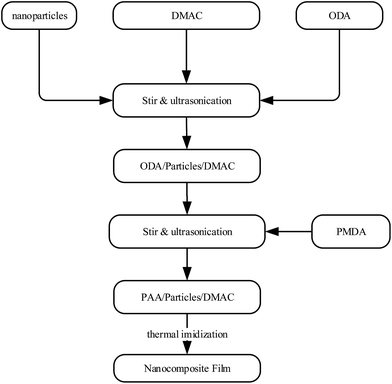
In situ polymerization was employed to prepare the polyimide matrix inorganic nanocomposite films. The experimental materials were as follows: 4,4′-ODA (oxy dianiline), PMDA (pyromellitic dianhydride), N,N-DMAC (dimethylacetamide), BaTiO3, Rutile TiO2, SiO2, α-Al2O3, Al2O3 and C2H6O. First, PMDA was added to the solution of 4,4′-ODA and N,N-DMAC to prepare the ployamic acid. Next, different nanoparticles were added to the prepared acid, which was then processed by paving membrane heat treatment and imidization. Fig. 1 shows the detailed preparation process of the polyimide matrix inorganic nanocomposite films.In this study, 32 polyimide matrix inorganic nanocomposite films with different weight ratios, sizes and thicknesses and doped with different inorganic nanoparticles (BaTiO3, Rutile TO2, SiO2, α-Al2O3 and Al2O3) were prepared. The film samples are listed in Table 1.
| Nanoparticles | Particle size (nm) | Doped proportion (wt%) | Film thickness (μm) |
|---|---|---|---|
| BaTiO3 | 100 | 10, 15, 20, 25, 30, 50, 60, 70 | 25 |
| Rutile TiO2 | 35 | 1, 3, 4, 5, 7 | 25 |
| SiO2 | 40 | 5, 10, 15, 20, 25 | 25 |
| SiO2 | 7 | 10, 15, 20, 25 | 30 |
| α-Al2O3 | 30 | 4, 8, 12, 16, 20, 24 | 30 |
| Al2O3 | 13 | 15, 20, 25 | 30 |
| PI | 0 | 0 | 25 |
Experiment condition & test devices
A broadband dielectric spectrometer (Novelcontrol, Germany) was used to obtain the dielectric spectrums of 40 sample pairs with the following settings: frequency 50 Hz, impedance 0.01 Ω to 100 TΩ and capacitance 1 fF to 1 F, with the accuracy of phase difference at 2 × 10⁻³ and the accuracy of dielectric loss (tan![[thin space (1/6-em)]](https://www.rsc.org/images/entities/char_2009.gif) δ) less than 10−5.
δ) less than 10−5.
A transmission electron microscope (Trcnai G2 F30) was used to observe the micro-structures of the prepared composite film samples at a resolution ratio of 0.205 nm and accelerating voltages of 50–300 kV.
FEI Quanta 200, at an accelerating voltage of 20 keV, was used to observe the surface and the fracture topographies of the composite film samples. The samples were directly observed under an electron microscope without surface treatment.
Results and discussion
Microstructure characterization
Both a transmission electron microscope and a scanning electron microscope were used to observe the microstructures of the surface and the fracture surface of the polyimide (PI) composite films, as shown in Fig. 2. Fig. 2a shows the microstructure of PI/Al2O3 (15 wt%) and Fig. 2b, c and d show the surface topographies of PI/BaTiO3 (20 wt%), PI/TiO2 (20 wt%) and PI/SiO2 (15wt%), respectively. Fracture and surface topographies of the different composite films were investigated. The results show that the inorganic nanoparticles have good dispersion in the 32 prepared films. These films have uniform thicknesses, and the particles bind closely with the PI matrix.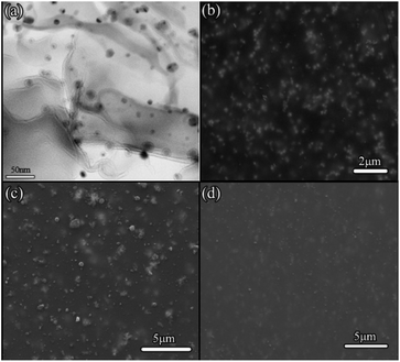 | ||
| Fig. 2 Microstructures of nanocomposite films (a) TEM image of the PI/Al2O3 15 wt%; (b) SEM image of the PI/BaTiO3 20 wt%; (c) SEM image of the PI/TiO2 20 wt%; (d) SEM image of the PI/SiO2 15 wt%. | ||
Dielectric loss results
Studies show that the physical properties of the doped inorganic nanoparticles are key factors that impact the dielectric loss of the composite films. On the basis of previous studies, this paper has built a library that contains 32 PI (polyimide) matrix composite films, with parameters such as inorganic nanoparticle type, dielectric constant, electrical resistivity, thermal conductivity, particle size, specific surface area and nanocomposite film thickness. The dielectric losses of the composite films in Table 1 are tested at room temperature at a frequency of 50 Hz, and the test results are shown in Table 2.| Sample | Type of nanoparticles | Input | Output | ||||||
|---|---|---|---|---|---|---|---|---|---|
| X1 | X2 | X3 | X4 | X5 | X6 | X7 | Y | ||
| a X1: dielectric constant of the nanoparticle; X2: electrical resistivity of the nanoparticle (Ω m); X3: film thickness (μm); X4: thermal conductivity of the nanoparticle (W cm−1 K−1); X5: doping ratio of the nanoparticle (wt%); X6: size of the nanoparticle (nm); X7: specific surface area of the nanoparticle (m2 g−1), and; Y: dielectric loss of the nanocomposite film. | |||||||||
| 1 | BaTiO3 | 1400 | 1 × 10⁵ | 25 | 0.50 | 10 | 100 | 12 | 0.00140 |
| 2 | BaTiO3 | 1400 | 1 × 10⁵ | 25 | 0.50 | 15 | 100 | 12 | 0.00200 |
| 3 | BaTiO3 | 1400 | 1 × 10⁵ | 25 | 0.50 | 20 | 100 | 12 | 0.00246 |
| 4 | BaTiO3 | 1400 | 1 × 10⁵ | 25 | 0.50 | 25 | 100 | 12 | 0.00276 |
| 5 | BaTiO3 | 1400 | 1 × 10⁵ | 25 | 0.50 | 30 | 100 | 12 | 0.00296 |
| 6 | BaTiO3 | 1400 | 1 × 10⁵ | 25 | 0.50 | 50 | 100 | 12 | 0.00652 |
| 7 | BaTiO3 | 1400 | 1 × 10⁵ | 25 | 0.50 | 60 | 100 | 12 | 0.01647 |
| 8 | BaTiO3 | 1400 | 1 × 10⁵ | 25 | 0.50 | 70 | 100 | 12 | 0.01839 |
| 9 | Rutile TiO2 | 100 | 9 × 10⁷ | 25 | 0.40 | 0 | 35 | 70 | 0.00177 |
| 10 | Rutile TiO2 | 100 | 9 × 10⁷ | 25 | 0.63 | 1 | 35 | 70 | 0.00165 |
| 11 | Rutile TiO2 | 100 | 9 × 10⁷ | 25 | 0.63 | 3 | 35 | 70 | 0.00199 |
| 12 | Rutile TiO2 | 100 | 9 × 10⁷ | 25 | 0.63 | 4 | 35 | 70 | 0.00156 |
| 13 | Rutile TiO2 | 100 | 9 × 10⁷ | 25 | 0.63 | 5 | 35 | 70 | 0.00278 |
| 14 | Rutile TiO2 | 100 | 9 × 10⁷ | 25 | 0.63 | 7 | 35 | 70 | 0.00283 |
| 15 | SiO2 | 1.56 | 1 × 10¹⁶ | 25 | 160 | 5 | 40 | 300 | 0.00150 |
| 16 | SiO2 | 1.56 | 1 × 10¹⁶ | 25 | 160 | 10 | 40 | 300 | 0.00200 |
| 17 | SiO2 | 1.56 | 1 × 10¹⁶ | 25 | 160 | 15 | 40 | 300 | 0.00180 |
| 18 | SiO2 | 1.56 | 1 × 10¹⁶ | 25 | 160 | 20 | 40 | 300 | 0.00150 |
| 19 | SiO2 | 1.56 | 1 × 10¹⁶ | 25 | 160 | 25 | 40 | 300 | 0.00160 |
| 20 | α-Al2O3 | 10 | 1 × 10¹⁴ | 30 | 4.10 | 4 | 30 | 25 | 0.00300 |
| 21 | α-Al2O3 | 10 | 1 × 10¹⁴ | 30 | 4.10 | 8 | 30 | 25 | 0.00450 |
| 22 | α-Al2O3 | 10 | 1 × 10¹⁴ | 30 | 4.10 | 12 | 30 | 25 | 0.00500 |
| 23 | α-Al2O3 | 10 | 1 × 10¹⁴ | 30 | 4.10 | 16 | 30 | 25 | 0.00700 |
| 24 | α-Al2O3 | 10 | 1 × 10¹⁴ | 30 | 4.10 | 20 | 30 | 25 | 0.00800 |
| 25 | α-Al2O3 | 10 | 1 × 10¹⁴ | 30 | 4.10 | 24 | 30 | 25 | 0.00850 |
| 26 | Al2O3 | 8 | 1 × 10¹⁴ | 30 | 29.31 | 15 | 13 | 100 | 0.00266 |
| 27 | Al2O3 | 8 | 1 × 10¹⁴ | 30 | 29.31 | 20 | 13 | 100 | 0.00285 |
| 28 | Al2O3 | 8 | 1 × 10¹⁴ | 30 | 29.31 | 25 | 13 | 100 | 0.00305 |
| 29 | SiO2 | 1.56 | 1 × 10¹⁶ | 30 | 160 | 10 | 7 | 350 | 0.00335 |
| 30 | SiO2 | 1.56 | 1 × 10¹⁶ | 30 | 160 | 15 | 7 | 350 | 0.00372 |
| 31 | SiO2 | 1.56 | 1 × 10¹⁶ | 30 | 160 | 20 | 7 | 350 | 0.00413 |
| 32 | SiO2 | 1.56 | 1 × 10¹⁶ | 30 | 160 | 25 | 7 | 350 | 0.00460 |
Ensemble learning prediction model
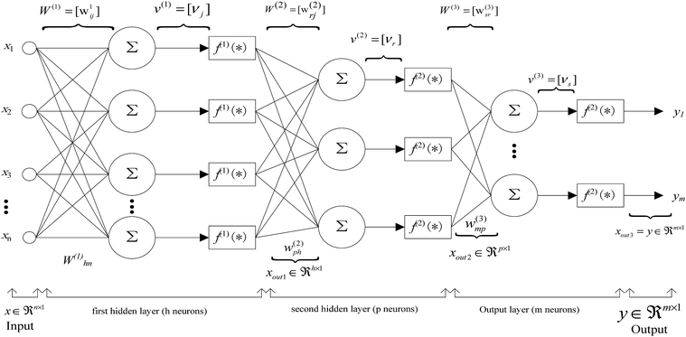
Ensemble learning has been proposed by many researchers as a solution to both the over-fitting and the low accuracy of model regression and classification. Currently, it is a hotspot in the fields of machine learning and intelligent computing.19–23 Ensemble learning can be used to convert a number of weak classifiers into a strong one. Common ensemble learning methods include boosting, bagging and random forest. Boosting constantly upgrades its weight during data extraction and corrects the dataset weight for the former misclassification such that a strong classifier or a strong regression model can be built. Bagging includes the weighting of multiple classifiers that are generated from a training set. As an improved version of boosting, random forest is stronger for regression and can prevent over-fitted predictions.Artificial neural networks have been widely used for predicting and identifying material properties in recent years.24–26 A multilayer perceptron (MLP) is a feedforward artificial neural network model that maps sets of input data onto a set of appropriate outputs.27 An MLP consists of three parts, which are the input layer, hidden layer and output layer. Fig. 3 is a standard three-layer feedforward MLP where i = 1, 2, …, n, j = 1, 2, …, h, r = 1, 2, …, p, and s = 1, 2, …, m. For each layer, there is a synaptic weight matrix that connects the former layer to the next layer. The definitions of a nonlinear input–output map and a nonlinear diagonal matrix are given as follows:
| f(l)(*) = diag[f(1)[*], f(2)[*], …, f(l)[*]] | (1) |
 the output of the first layer is as follows:
| xout1 = f(1)[ν(1)] = f(1)[W(1)x] | (2) |
If eqn (2) is taken as the input of the second layer, then the output of the second layer is as follows:
| xout2 = f(2)[ν(2)] = f(2)[W(2)xout1] | (3) |
If eqn (3) is taken as the input of the third layer, then the output of the third layer is as follows:
| y = xout3 = f(3)[ν(3)] = f(3)[W(3)xout2] | (4) |
Substituting eqn (2) into (3) and (4), we obtain the final network:
| y = f(3)[W(3)f(2)[W(2)f(1)[W(1)x]]] = Ω[x] | (5) |
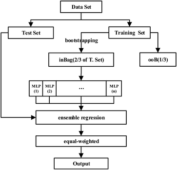
The RF (random forests) algorithm was proposed by Leo Breiman in 2001.28 The algorithm contains a multitude of decision trees, and random forests are generated from a number of combined optimization decision trees. RF is a fast and efficient machine learning method for classification and regression. It has many advantages. It can effectively prevent over-fittings, quickly process high dimensional data, and maintain high accuracy when the dataset is not complete. By virtue of the idea of random forests, we use an MLP (multilayer perceptron) neural network to replace the decision tree to construct an RF-MLP (random forest and multilayer perceptron) model, as shown in Fig. 4. Calculation steps of the RF-MLP model are as follows:
Step 1: Randomly extracting N samples from the training samples of the nanocomposite films;
Step 2: Randomly extracting K samples from the explanatory variables and using the Gini value to select the variable that leads to the minimal variability of the divided internal subset;
Step 3: Using the variable obtained in step 2 to divide the training set into two subsets;
Step 4: Repeating step 3 and training the MLP by using the divided subsets;
Step 5: Averaging the MLP regression models.
Model assessment
Many indexes can be used to assess the prediction performance, such as MAPE (mean absolute percentage error), MAE (mean absolute error), RMSE (root mean squared error), CC (correlation coefficient), RAE (relative absolute error) and RRSE (root relative squared error), etc. In this study, the four indexes, CC, MAE, RMSE and RRSE, were used.The CC (correlation coefficient) represents how close the linear regression relation between fi (independent variable) and yi (response variable) is. It is directly proportional to prediction accuracy.
MAE (mean absolute error) is the diversity between the predicted value and the measured value. It is inversely proportional to prediction accuracy. MAE can be expressed as follows:
 | (6) |
RMSE (root mean squared error) is inversely proportional to prediction accuracy. In other words, the smaller the value of RMSE is, the more accurate the predictor will be. It is expressed as follows:
 | (7) |
The expression of RRSE (root relative squared error) is as follows:
 | (8) |
It is inversely proportional to prediction accuracy, which means that the smaller the value of RSSE is, the more accurate the predictor will be.
Results of the prediction model
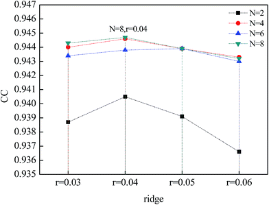
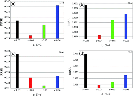
The computer was a Mac Book Pro Intel I7 CPU with 16 GB DDR-RAM. The programming software used was Java and WEKA.29 A 10-fold cross validation was used for the accuracy test. The dataset was divided into ten subsets. Nine subsets were taken as the training set and one subset was used for test. The mean value of the 10 prediction accuracies was taken as the final accuracy. Model parameters include the number of basic regressions, attribute, r (ridge) and N (number of neurons). Here, the MLP neural network has ten basic regressions. For tuning the value manually, Fig. 5 shows the CC curve when both N and r are changing. When N = 8 and r = 0.04, CC reached its maximum value of 0.9447; in this case, the regression performance was the best and the prediction accuracy was the highest. Fig. 6, 7, and 8 show the curves of the MAE, RSME and RRSE, respectively. When N = 8 and r = 0.04, the MAE, RMSE and RRSE reached their minimum values of 0.0007, 0.0014 and 34.89%, respectively, in which situation, the prediction accuracy of the model was the highest. The above data show that when the number of the MLP regression is 10 and N = 8 and r = 0.04, the model had the highest prediction accuracy.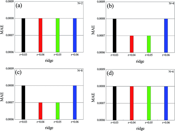 | ||
| Fig. 6 Variation of MAE and N; (a) N = 2, r changes from 0.003 to 0.06; (b) N = 4, r changes from 0.003 to 0.06; (c) N = 8, r changes from 0.003 to 0.06; (d) N = 6, r changes from 0.003 to 0.06. | ||
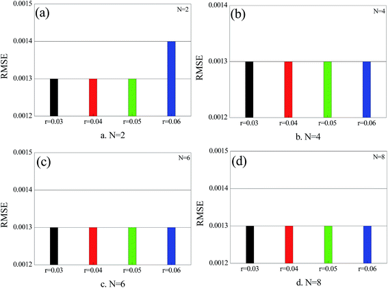 | ||
| Fig. 7 Variation of RMSE and N; (a) N = 2, r changes from 0.003 to 0.06; (b) N = 4, r changes from 0.003 to 0.06; (c) N = 6, r changes from 0.003 to 0.06; (d) N = 8, r changes from 0.003 to 0.06. | ||
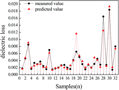
Attribute selection, also called dimensionality reduction, is a key factor to control the prediction accuracy of the model. Common attribute selection modes include all-attribute, principal component analysis (PCA) and the Haar wavelet transform. In the RF-MLP model, the three modes are experimentally compared. Table 3 lists the comparison results of the prediction accuracy when N = 8 and r = 0.04. As Table 3 shows, the CC value is 0.9447 in the principal component analysis mode, which is higher than those in the other two modes. In the principal component analysis mode, the MAE, RMSE and RRSE are 0.0007, 0.0013 and 32.0972%, respectively, which are all smaller than those in the all-attribute and Haar wavelet transform modes. Fig. 9 shows the comparison between the predicted values and the measured values when the model was set at the optimal parameters (N = 8, r = 0.04, principal component and 10-fold cross validation). The well-fitting curves show that the model is effective to predict the dielectric losses of the nanocomposite films.
| Assessment | Normal | PCA | Haar wavelet |
|---|---|---|---|
| CC | 0.9327 | 0.9447 | 0.9419 |
| MAE | 0.0009 | 0.0007 | 0.0008 |
| RMSE | 0.0014 | 0.0013 | 0.0013 |
| RRSE (%) | 35.2677 | 32.0972 | 32.8783 |
Model comparison
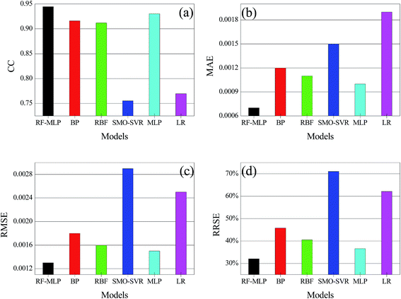
For further verification, the RF-MLP model was experimentally compared with the LR (linear regression),30 BP (backpropagation) neural network,31 RBF (radial basis function) neural network,32 SVR (support vector regression)33 and MLP (multilayer perceptron) neural network34 under the same conditions. The comparison results are shown in Table 4 and Fig. 10. As shown in Fig. 10a, the CC value of the RF-MLP model is 0.962, which is higher those of LR, RBF, MLP and SVR. This proves that the linear regression relation of the RF-MLP model is better than that of the other five models. According to Fig. 10b, c and d, the MAE, RMSE and RRSE values of the RF-MLP model are 0.0007, 0.0013 and 32.0972%, respectively, which are all smaller than those of the other five models. This proves that the prediction accuracy of the RF-MLP model is better than that of the other five models.| Assessment | RF-MLP | BP | RBF | SMO-SVR | MLP | Linear regression |
|---|---|---|---|---|---|---|
| CC | 0.9447 | 0.9159 | 0.9120 | 0.7555 | 0.9302 | 0.7699 |
| MAE | 0.0007 | 0.0012 | 0.0011 | 0.0015 | 0.0010 | 0.0019 |
| RMSE | 0.0013 | 0.0018 | 0.0016 | 0.0029 | 0.0015 | 0.0025 |
| RRSE | 32.0972% | 45.8046% | 40.5254% | 71.1128% | 36.5720% | 62.1629% |
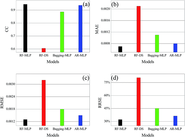
Table 5 and Fig. 11 show the results of the comparison between the RF-MLP model and other ensemble learning models, including the RF (random forest)-decision stump, bagging-MLP and AR (Additive Regression)-MLP. As seen in Fig. 11a, the CC value of the RF-MLP model is 0.9447, which is higher than that of the other three models. Fig. 11b, c and d show that the MAE, RMSE and RRSE values of the RF-MLP model are 0.0007, 0.0013 and 32.0972%, respectively, which are all smaller than those of the other three models. Therefore, compared with other ensemble learning models, the RF-MLP model could generate smaller error and better performance in predicting the dielectric losses of the nanocomposite films.
| Assessment | RF-MLP | RF-decision stump | Bagging-MLP | Additive regression-MLP |
|---|---|---|---|---|
| CC | 0.9447 | 0.6054 | 0.8861 | 0.9373 |
| MAE | 0.0007 | 0.0021 | 0.0011 | 0.0008 |
| RMSE | 0.0013 | 0.0032 | 0.0018 | 0.0015 |
| RRSE | 32.0972% | 80.5834% | 45.0949% | 36.2929% |
Robustness of the prediction model
In ref. 18, the GRNN (generalized regression neural network) was used to predict the friction coefficient of deposited Cr1−xAlxC films, and the seven control factors selected in experiments were the chromium and aluminium target current, argon and acetylene flow rate, negative bias voltage, DC pulse frequency, and sputtering time. To verify the generality and the robustness of the model in this paper, we use the same sample data and condition in ref. 18 to make an experimental comparison, as shown in Table 6. The optimized parameters of the RF-MLP model are as follows. The random seed is 1, the number of the basic regressions is 10, the attribute is PCA, r (ridge) is 0.01, and N (the number of the neurons) is 10. When the RF-MLP model was used to predict the friction coefficient of deposited Cr1−xAlxC films, the CC value was 0.896 and the RMSE value was 0.053. These values are far smaller than those in ref. 18, which indicates that the RF-MLP model is more accurate than the model in ref. 18 in predicting the friction coefficient of deposited Cr1−xAlxC films. As proven by the comparison, the RF-MLP model shows both generality and robustness when used to predict properties of other films.| RF-MLP | GRNN18 | |
|---|---|---|
| CC | 0.896 | — |
| RMSE | 0.053 | 0.36 |
Conclusions
In this study, the method of in situ polymerization was employed to prepare 32 polyimide matrix nanocomposite films that have different weight ratios, sizes and thicknesses and doping ratios of inorganic nanoscale particles. Dielectric losses of the 32 prepared films were measured as well. Based on the results of the experiment, the RF-MLP ensemble learning model for predicting the dielectric losses of the polyimide nanocomposite films is proposed. By using the random forest method, we convert 10 multilayer perceptron neural networks into a strong prediction model which is efficient in predicting the dielectric losses of the polyimide nanocomposite films. The following conclusions are obtained based on the experimental data:(1) The 10-fold cross validation was used to predict the dielectric losses of 32 polyimide nanocomposite films. For the prediction results, the CC was 0.9447, the MAE was 0.0007, the RMSE was 0.0013, and the RRSE was 32.0972%, which indicate that the RF-MLP model is efficient in predicting such dielectric losses.
(2) The comparison experiment shows that the CC value of the RF-MLP model is higher than that of the linear regression, backpropagation neural network, radial basis function neural network, support vector regression and multilayer perceptron neural network. In addition, compared with the other models, the RF-MLP model has smaller MAE, RMSE and RRSE values and better prediction parameters.
(3) If compared with other ensemble learning methods, such as bagging, boosting and RF-decision stump, the RF-MLP model has a higher CC value but lower MAE, RMSE and RRSE values when used to predict the dielectric losses of polyimide nanocomposite films. This indicates that the RF-MLP model is more accurate for dielectric loss prediction.
(4) The results show that the RF-MLP model is applicable not only to predicting the dielectric loss of the polyimide nanocomposite films but also to predicting the friction coefficient of deposited Cr1−xAlxC films with prediction accuracy than other models. In addition, the RF-MLP model exhibits considerable robustness.
For further studies, we plan to use other ensemble learning methods to predict corona resistance, dielectric constant and thermal weight losses of polyimide matrix nanocomposite films to provide an efficient, fast and reliable method for predicting the dielectric properties of new nano-materials. In this paper, we have only discussed the dielectric losses of polymer-based composites with orientation polarization. In further research, we will focus on the applicability of this model for poly-anion-type materials, such as SiO2 and KH2PO4.
Acknowledgements
This article has obtained the support of the National Natural Science Foundation of China (51077028, 51307046, 201501030401), Fund of the State Ethnic Affairs Commission of the People's Republic of China (14DLZ011), the Doctoral Scientific Research Foundation of Liaoning (201601084), the Fundamental Research Funds for the Central Universities, and the Doctoral Scientific Research Foundation of Dalian Nationalities University. Authors also gratefully acknowledge the helpful comments and suggestions of the reviewers who improved the presentation. The authors are also grateful to Dr Feng Yu and Dr Wang li-kun for polishing and modifying the English language for this paper.Notes and references
- C. R. Yates and W. Hayes, Eur. Polym. J., 2004, 40, 1257–1281 CrossRef CAS
.
- M. S. Zheng, J. W. Zha, Y. Yang, P. Han, C. H. Hu and Z. M. Dang, Appl. Phys. Lett., 2016, 109, 072902 CrossRef
.
- E. R. Thapaliya, Y. Zhang and F. M. Raymo, J. Mater. Chem. C, 2017, 5, 1179–1183 RSC
.
- D. Gao, Z. H. Chen, J. Y. Huang, W. F. Zhang, C. Y. Wei, Z. Z. Lin, D. Z. Li and G. Yu, J. Mater. Chem. C, 2017, 5, 3568–3578 RSC
.
- M. B. H. Othman, Z. Ahmad, H. M. Akil, M. R. Zakaria and F. Ullah, Mater. Des., 2015, 82, 98–105 CrossRef CAS
.
- Q. Y. Tang, Y. C. Chan and K. Zhang, Sens. Actuators, B, 2011, 152, 99–106 CrossRef CAS
.
- S. F. Wang, Y. R. Wang, K. C. Cheng and S. H. Chen, J. Mater. Sci.: Mater. Electron., 2010, 21, 104–110 CrossRef CAS
.
- H. Guo, J. H. Yin, J. Y. Zhao, Y. Y. Liu, L. Yao and X. Xia, J. Comput. Theor. Nanosci., 2015, 12, 890–893 CrossRef CAS
.
- Y. Feng, J. H. Yin, M. H. Chen, X. X. Liu, B. Su and W. Fei, IEEE Trans. Dielectr. Electr. Insul., 2014, 21, 1501–1508 CrossRef CAS
.
- W. Ling, Q. Xia, L. Yan, C. Wang, M. Cao and L. Liu, Polym. Polym. Compos., 2014, 22, 123–127 CAS
.
- H. Ahmadizadegan, RSC Adv., 2016, 6, 108 RSC
.
- M. Davoody, M. Sadeghi, M. Naghsh and A. Moheb, RSC Adv., 2016, 6, 23746–23759 RSC
.
- A. Bahramian, Surf. Interface Anal., 2013, 45, 1727–1736 CrossRef CAS
.
- Y. D. Ko, P. Moon, C. E. Kim, M. H. Ham, M. K. Jeong, A. Garcia-Diaz, J. M. Myoung and I. Yun, Surf. Interface Anal., 2013, 45, 1334–1339 CrossRef CAS
.
- M. M. Nobrega, E. Bona and F. Yamashita, Mater. Sci. Eng., C, 2013, 33, 4331–4336 CrossRef CAS PubMed
.
- M. Payandehdoost, N. Amanifard, M. Naghashnejad and H. M. Deylami, Heat Transf. Res., 2014, 45, 643–657 CrossRef
.
- M. Piliougine, D. Elizondo, L. Mora-López and M. Sidrach-de-Cardona, Appl. Energy, 2013, 112, 610–617 CrossRef
.
- Y. S. Yang, J. H. Chou, W. Huang, T. C. Fu and G. W. Li, Appl. Soft Comput., 2013, 13, 109–115 CrossRef
.
- I. Ahmed, R. Ali, D. Guan, Y. K. Lee, S. Lee and T. Chung, Expert Syst. Appl., 2015, 42, 1065–1073 CrossRef
.
- S. Wang, Y. Yin, G. Cao, B. Wei, Y. Zheng and G. Yang, Neurocomputing, 2015, 149, 708–717 CrossRef
.
- Z. H. Zhou, IEEE Trans. Knowl. Data Eng., 2014, 26, 1819–1837 CrossRef
.
- M. Seera, C. P. Lim, S. Nahavandi and K. L. Chu, Expert Syst. Appl., 2014, 41, 4891–4903 CrossRef
.
- D. Guan, W. Yuan, Y. K. Lee, K. Najeebullah and M. K. Rasel, IETE Technical Review, 2014, 31, 190–198 CrossRef
.
- H. Akbarpour, M. Mohajeri and M. Moradi, Comput. Mater. Sci., 2013, 79, 75–81 CrossRef CAS
.
- H. Guo, J. H. Yin, J. Y. Zhao, Y. Y. Liu, L. Yao and X. Xia, J. Comput. Theor. Nanosci., 2015, 12, 886–889 CrossRef CAS
.
- S. E. Restrepo, S. T. Giraldo and B. J. Thijsse, Comput. Mater. Sci., 2014, 86, 170–173 CrossRef
.
- A. Samolov, S. Dragović, M. Daković and G. Bačić, J. Environ. Radioact., 2014, 137, 198–203 CrossRef CAS PubMed
.
- L. Breiman, Mach. Learn., 2001, 45, 5–32 CrossRef
.
- I. H. Witten, E. Frank, M. A. Hall and C. J. Pal, Data Mining: Practical Machine Learning Tools and Techniques, Morgan Kaufmann, 2016 Search PubMed
.
- P. Y. Lai and M. S. Lee Stephen, Ann. Inst. Stat. Math., 2013, 65, 105–124 CrossRef
.
- Y. Lou, W. Wu and L. Li, J. Mater. Eng. Perform., 2012, 21, 1133–1140 CrossRef CAS
.
- M. Contreras, S. Nagarajaiah and S. Narasimhan, Smart Mater. Struct., 2011, 20, 035013 CrossRef
.
- H. Guo, J. H. Yin, J. Y. Zhao, Z. Y. Huang and Y. Pan, Int. J. Mater. Prod. Technol., 2014, 49, 5–17 CrossRef
.
- N. Kucuk, S. R. Manohara, S. M. Hanagodimath and L. Gerward, Radiat. Phys. Chem., 2013, 86, 10–22 CrossRef CAS
.
| This journal is © The Royal Society of Chemistry 2017 |

