Read-across predictions of nanoparticle hazard endpoints: a mathematical optimization approach

Abstract

In the present study, a novel read-across methodology for the prediction of toxicity related end-points of engineered nanomaterials (ENMs) is developed. The proposed method lies in the interface between the two main read-across approaches, namely the analogue and the grouping methods, and can employ a single criterion or multiple criteria for defining similarities among ENMs. The main advantage of the proposed method is that there is no need of defining a prior read-across hypothesis. Based on the formulation and the solution of a mathematical optimization problem, the method searches over a space of alternative hypotheses, and determines the one providing the most accurate read-across predictions. The procedure is automated and only two parameters are user-defined: the balance between the level of predictive accuracy and the number of predicted samples, and the similarity criteria, which define the neighbors of a target ENM.

---

1 Introduction

The impact of nanotechnology is escalated with the development of novel engineered nanomaterials (ENMs) and their use in industrial applications and commercial products.¹ However, current research in the nanotoxicity field raises awareness concerning the potential adverse effects of the exposure of living organisms in ENMs, including membrane rupture, DNA damage, oxidative stress and cell death.^2–4 Therefore, prior to their broad release into the market, great effort should be placed into the development of methods for ENM characterization, as well as for the assessment of environmental and human health risks caused by the exposure to ENMs.⁵

A complete and systematic experimental approach for the risk assessment of all variants of an ENM is practically impossible both in terms of time and resources, taking into account the amount and the variety of ENMs entering the market or already available. At the same time, given the ethical questions and the legislative requirements, animal testing should be reduced and performed only under strict conditions.^5–7

Over the past few years, the nanosafety community has encouraged the development of alternative non-testing methods for the toxicological investigation of ENMs introducing in vitro and in silico methods. The so called “nanoinformatics” field includes novel, computational approaches which can produce reliable predictions for the toxic and biological behavior of ENMs. These computer-aided methods aim to contribute to the prioritization of ENMs and to support the regulatory decision-making. One successful approach is the adaptation of the quantitative structure–activity relationship (QSAR) modeling methodologies⁸ to the special requirements of ENMs, which are due to their complex structures. The produced models are presented in the literature as nano-QSARs or QNARs (quantitative nanostructure–activity relationship) models. Comprehensive reviews of nano-QSAR modelling methods and produced predictive models have been published recently in the literature.^9,10 A repository of nano-QSAR models is included in the final report of the Nanocomput project and is freely available through the European Commission Science Hub.¹¹

However, in order to ensure the functionality of the QNAR approaches, sufficiently large (more than 20 samples) and diverse datasets should be provided.^5,12 European Chemicals Agency (ECHA) through the Read-Across Assessment Framework (RAAF) has introduced the alternative read-across non-testing strategy,^13,14 for the prediction of ENM toxicity, especially in the case of absence of sufficient large datasets for the development of reliable nano-QSAR models.⁵ The read-across concept is based on the empirical knowledge that similar materials may exhibit comparable properties, thus the estimation of the hazardous effects of non-tested ENMs can be achieved using data within a group of comparable ENMs.^5,15,16

There are two approaches regarding the read-across framework, supported by ECHA and OECD; the analogue and the category/grouping approach. The definitions of the two approaches slightly differ between ECHA and OECD,¹⁷ however their eminent characteristics are presented in Table 1.

Table 1 Overview of the two read-across approaches^13,17

Analogue approach	Grouping approach
Employed between a small number of structurally similar substances (source and target substances)	Employed between several substances that have structural similarity
No trend or regular pattern in the properties	A trend or a regular pattern is expected (in order to accept or reject the grouping hypothesis)
Evaluation of each sample independently	Evaluation of the category as a whole
Worst case: single source substance (one neighbor)	Worst case: the strength of effects in a target sample within the group is expected to be lower than the strength of effects observed for the source sample

---

In the analogue approach the prediction is limited to a small area of the data space; one source ENM can be used for the endpoint estimation for a single or more target ENMs, or two or more source ENMs can be used to make predictions for a single or several target ENMs. The read-across methodologies apply an interpolation strategy “locally” among similar samples which, depending on the provided data – numerical or discrete –, can be quantitative or qualitative.¹⁸ The methods for the prediction of each endpoint range from simple average value calculations, or simple linear interpolations to more complicated methods applying QSAR methods locally (e.g. k-nearest neighbor, partial least squares, random forests).^5,19

In the categorical approach, the ENM samples are organized into groups of similar compounds. Groups are formed considering structural similarities between samples, and it is assumed that due to these similarities, the biological or toxic activity of the ENMs within a group follows a regular pattern. Groups of ENMs can be further divided into subgroups based on interdependencies in nanodescriptors and the formation of these subgroups can be “tuned” in order to gain satisfactory predictions.^20,21 Other studies have investigated alternative grouping possibilities including principal component analysis (PCA),²² linear discriminant analysis (LDA),²¹ two-dimensional hierarchical clustering¹⁸ or considering the ENM mode-of-action.⁶ For the estimation of the endpoint of a target ENM in a group, the analogue approach can be applied.

Several read-across tools and methods for the preliminary hazard assessment of ENMs have been proposed in the literature.¹⁶ Gajewicz et al.⁵ proposed a novel quantitative read-across approach for data gap filling of ENMs using the one-point-slope, the two-point formula and the equation of a plane passing through three points. Their nano-QRA model proved to have high predictive capabilities, when tested with the same dataset used by Puzyn et al.²³ Helma et al.¹⁹ introduced recently the nano-lazar framework for ENM read-across predictions. The similarity levels for the selection of neighbors are based on the Tanimoto/Jaccard index and on weighted cosine similarity. Three local regression algorithms are available: weighted local average, weighted partial least squares regression and weighted random forests. Helma et al. tested the performance of their methods using the dataset initially presented by Walkey et al.²⁴ consisting of 121 gold and silver ENMs that are characterized by physicochemical descriptors, the protein corona fingerprints (PCF) and by MP2D fingerprints calculated for core and coating compounds with defined chemical structures. They reported R² values equal to 0.68, for the prediction of the cell association with human A549 cells, using only the protein corona fingerprints and the weighted random forest algorithm, in a 10-fold cross validation scheme. Varsou et al.²⁰ presented the toxFlow web application, which integrates physicochemical, omics and biology information data for read-across toxicity prediction of ENMs. Neighbor selection is based either on the cosine similarity between ENMs or a distance metric (Euclidean, Manhattan). Using only the gold ENMs of the Walkey et al.²⁴ study and performing enrichment analysis to the PCF data prior to read-across, Varsou et al. reported R² values of 0.97 in the toxicity prediction, by employing a weighted average algorithm and a leave-one-out validation scheme.

ECHA has recently presented a systematic ENM specific workflow for grouping and read-across in the document titled “Recommendations for nanomaterials applicable to the guidance on QSARs and grouping”.²⁵ This workflow was slightly modified by Lamon et al.¹⁶ and Aschberger et al.²⁶ who presented a simplified version consisting of four steps: (1) identify the (nano)forms of the substance, (2) gather the available data, evaluate them for adequacy and reliability and build the data matrix, (3) develop a grouping hypothesis and assign the source analogues to groups, (4) assess the applicability of the grouping hypothesis and fill data gaps. The simplified workflow was used to develop case studies for the read-across prediction of hazard endpoints of nanoforms of TiO₂ and of Multi-Walled Carbon NanoTubes (MWCNTs) respectively. The first of these studies has been released as an official OECD document.²⁷

The read-across workflow proposed by ECHA assumes a hypothesis, which is evaluated and assessed in terms of its adequacy to fill data gaps. The read-across hypothesis may involve both the selection of the most informative descriptors that can predict the endpoint of interest and the definition of the source ENMs, which can be considered as neighbors to the target ENM. This procedure is iterated in a trial-and-error fashion until a hypothesis producing successful read-across predictions is determined. The procedure is time-consuming and due to the complexity of the problem, it does not guarantee that the produced read-across model is optimal.

In this paper we are presenting a novel read-across methodology, which automates the procedure of searching for the optimal read-across hypothesis. The proposed method considers both key components of the read-across procedure as optimization parameters: variable selection and the boundaries that define the neighborhood of the query ENM, for which a read-across prediction is sought. Another advantage of the proposed methodology is that it takes into account the multi-perspective characterization of ENMs by grouping ENM descriptors into categories (e.g. physicochemical, biological, quantum mechanical, image or biokinetics) and by using multiple similarity criteria for defining neighbors to the target ENM. The proposed method is based on the formulation of a mathematical Mixed Integer Non Linear Programming (MINLP) problem. For the solution of this problem, we develop an innovative Genetic Algorithm (GA), because conventional MINLP solvers fail to solve efficiently the optimisation problem.

2 Methods

2.1 Development of the MINLP problem

For the development of a robust and reliable read-across workflow for the prediction of ENM undesired properties, we focused on two separate goals: first, the reduction of the available dataset, by removing the variables that add noise rather than useful information to the analysis. Second, the definition of the neighbor boundaries which indicate the source ENMs that are considered similar to the target ENM. These two different goals can be achieved simultaneously through the development of an MINLP problem, where the objective is to minimize the mean squared error (MSE) between the experimental values and the produced predictions with respect to selecting the most informative descriptors and defining the neighbor boundaries. The problem is explained in detail below.

2.1.1 Available data. The methodology assumes the availability of a dataset containing the values of L descriptors and the endpoint for N ENMs. The data are first scaled using a standardisation (e.g. Gaussian normalization) or a normalisation (e.g. min–max) method, to ensure that scaled descriptors contribute equally to the overall prediction analysis.²⁸ The dataset is denoted by {x_i, y_i}, i = 1, … N, where x_i = {x_i,1, x_i,2, … x_i,L} is a vector containing the values of the L descriptors and y_i is the endpoint value of the ith ENM.

2.1.2 Set of variables. The main results of the solution of the MINLP problem are the following:

• : a binary variable indicating if the descriptor is selected or not, .

• thr: a continuous variable that defines a threshold for the selection of neighbor ENMs. Only if the Euclidean distance between two ENMs is equal to or less than thr, these two ENMs are considered as neighbors.

A number of additional variables are used for the construction of the MINLP problem:

• dist_i,j: a continuous variable containing the Euclidean distance between ENMs i and j, i = 1, …, N, j = 1, …, N.

• neib_i,j: a binary variable taking the value of 1 if ENMs i and j are neighbors and 0 if they are not, i = 1, …, N, j = 1, …, N.

• pred_i: a binary variable taking the value of 1, if ENM i has at least one neighbor and 0 if it has no neighbors, i = 1, …, N.

• ŷ_i: a continuous variable containing the predicted read-across endpoint value for the ith ENM, i = 1, …, N.

2.1.3 Mathematical formulation. The mathematical formulation of the optimisation problem consists of a set of well-defined constraints that should be satisfied by the solution of the problem and the objective function to be minimised.

Eqn (1) computes the Euclidean distance between all pairs of ENMs considering only the selected descriptors:

The following set of equations ensures that two ENMs i and j are considered as neighbors only if their Euclidean distance dist_i,j is equal to or lower than the threshold. In this case the corresponding binary variable neib_i,j takes the value of 1, otherwise the value of 0 is assigned to this variable. In eqn (2) and (3), m is a very small positive real number (equal to 10⁻³):

neib_i,j ≥ m(thr − dist_i,j), ∀ i,j ∈ {1, …, N}, i ≠ j (2)

1 − neib_i,j ≥ −m(thr − dist_i,j), ∀ i,j ∈ {1, …, N}, i ≠ j (3)

neib_i,i = 0, ∀ i ∈ {1, …, N} (4)

Eqn (5) computes the read-across predictions as weighted averages of the endpoint values of neighbor ENMs:

For ENMs without any neighbor, read-across predictions are not possible. An additional set of constraints (eqn (6)–(8)) guarantees that the percentage of ENMs with at least one neighbor is greater than or equal to a predefined percentage denoted by predFactor. In these equations, pred_i is a binary variable that becomes equal to 1, when a read-across prediction is achieved for the ith ENM, and 0, if no prediction is possible:

pred_i ≥ neib_i,j, ∀ i ∈ {1, …, N},∀ j ∈ {1, …, N} (7)

Objective function: the objective function to be minimized (eqn (9)) is the MSE between the end-point read-across predictions and the actual endpoint values over all the ENMs with at least one neighbor.

2.2 Extension of the MINLP problem to multiple similarity criteria

Due to the complex structure of ENMs, different types of data and descriptors are often used for ENM characterization. These may include physicochemical, biological, quantum-mechanical, image, biokinetic descriptors etc. In a previous study,²⁰ we demonstrated the use of two similarity criteria for defining different thresholds and for selecting the neighbors if different types of data are available. In this approach, distances can be calculated between all substances separately for the different types of data, and two ENMs are considered as neighbors if both distances are lower than the corresponding thresholds. The MINLP formulation described before is extended in this subsection to account for multiple similarity criteria. For brevity and for simplified notation, the extended formulation is presented for two similarity criteria. Inclusion of additional criteria is trivial.

2.2.1 Available data. The descriptors are grouped into sets A and B containing L_A and L_B descriptors respectively. The dataset is presented to the algorithm in the form {xA_i, xB_i, y_i}, i = 1, …, N, where xA_i = {xA_i,1, xA_i,2, …, xA_i,LA}, and xB_i = {xB_i,1, xB_i,2, …, xB_i,LB}, i = 1, …, N.

2.2.2 Set of variables. The main outcomes of the MINLP problem are:

• : a binary variable indicating if the descriptor in group A is selected or not, .

• : a binary variable indicating if the descriptor in group B is selected or not, .

• thr_A, thr_B: two continuous variables defining the threshold for the selection on neighboring ENMs for the two similarity criteria. Only if both Euclidean distances between two ENMs are equal to or less than the respective thresholds, these two ENMs are considered as neighbors.

The following additional variables are used for the construction of the MINLP problem:

• distA_i,j, distB_i,j: two continuous variables containing the Euclidean distance between ENMs i and j for the two similarity criteria, i = 1, …, N, j = 1, …, N.

• neibA_i,j, neibB_i,j: two binary variables taking the value of 1 if ENMs i and j are neighbors with respect to similarity criteria A or B and 0 if they are not, i = 1, …, N, j = 1, …, N.

• neib_i,j: a binary variable taking the value of 1 if ENMs i and j are neighbors and 0 if they are not, i = 1, …, N, j = 1, …, N.

• pred_i: a binary variable taking the value of 1, if ENM i has at least one neighbor and 0 if it has no neighbors, i = 1, …, N.

• ŷ_i: a continuous variable containing the predicted read-across endpoint value for the ith ENM, i = 1, …, N.

2.2.3 Mathematical formulation. The set of constraints is similar to the previous formulation.

The next equations (eqn (10) and (11)) compute the Euclidean distances between all pairs of ENMs taking into account only the selected descriptors for groups A and B.

The following set of equations ensure that two ENMs are considered as neighbors with respect to the different similarity criteria only if the Euclidean distances are lower than the respective threshold. In this case the corresponding binary variable takes the value of 1, otherwise the value of 0 is assigned to this variable. In eqn (12), (13), (15) and (16)m is a very small positive real number:

neibA_i,j ≥ m(thr_A − distA_i,j), ∀ i,j ∈ {1, …, N}, i ≠ j (12)

1 − neibA_i,j ≥ −m(thr_A − distA_i,j), ∀ i,j ∈ {1, …, N}, i ≠ j (13)

neibA_i,i = 0, ∀ i ∈ {1, …, N} (14)

neibB_i,j ≥ m(thr_B − distB_i,j), ∀ i,j ∈ {1, …, N}, i ≠ j (15)

1 − neibB_i,j ≥ −m(thr_B − distB_i,j), ∀ i,j ∈ {1, …, N}, i ≠ j (16)

neibB_i,i = 0, ∀ i ∈ {1, …, N} (17)

The set of equations, eqn (18)–(20) define two ENMs i and j as neighbors if they satisfy both similarity criteria, i.e. only if both neibA_i,j and neibB_i,j are equal to 1.

neib_i,j ≥ neibA_i,j + neibB_i,j − 1, ∀ i,j ∈ {1, …, N} (18)

neib_i,j ≤ neibA_i,j, ∀ i,j ∈ {1, …, N} (19)

neib_i,j ≤ neibB_i,j, ∀ i,j ∈ {1, …, N} (20)

Eqn (21) computes the read-across predictions as weighted averages of the endpoint values of neighbor ENMs by selecting one distance metric (here we assume the metric based on group A):

Constraints 6, 7, and 8 are used again to guarantee that the percentage of ENMs with at least one neighbor is greater than or equal to a predefined percentage denoted by predFactor.

Objective function: the objective function is the same as in the previous MINLP formulation (eqn (9)).

3 Solution strategy

The above described MINLP problems cannot be solved efficiently by conventional optimization methods. For the solution of the problem, we developed a novel evolutionary algorithm based on the concept of Genetic Algorithms (GAs) which is described in detail in this section. GAs have been used successfully for the variable subset selection in different optimization problems.²⁹

The development of GAs is “bio-inspired” from the principles of species evolution, and is based on the concept that living organisms are examples of successful optimization. The operational parameters of the GAs are summarised next and are directly linked to the biological processes of selection, crossover and mutation of genes:

• Potential solution (chromosome): the chromosome contains a sequence of genes with a length equal to the total number of variables.

• Group of potential solutions (population): a group of chromosomes (an even number).

• Iterations (generations): a number of cycles of selection, crossover and mutation between the potential solutions, leading to an optimal solution.

• Fitness evaluation (selection): a process of selection of chromosomes based on their calculated fitness. The reproduction of the fittest chromosomes in the next generation must be assured.

• Combination of two potential solutions (crossover): reproduction operator is employed to exchange genes between two chromosomes, in a random point of crossover.

• Alteration of a potential solution (mutation): a process of alteration of the crossovered chromosomes. According to a predefined probability value, the procedure inverts the value of each gene: 0 becomes 1 and vice versa (uniform mutation).³⁰

• Ensuring desirable evolution (elitism): during the creation of a new population with different biological processes, there is a chance of losing the chromosome with the highest score. This method forces the best chromosome to be included in the new population.

• Optimal solution (genome): a chromosome containing the combination of genes among the generations that leads to the optimal solution.

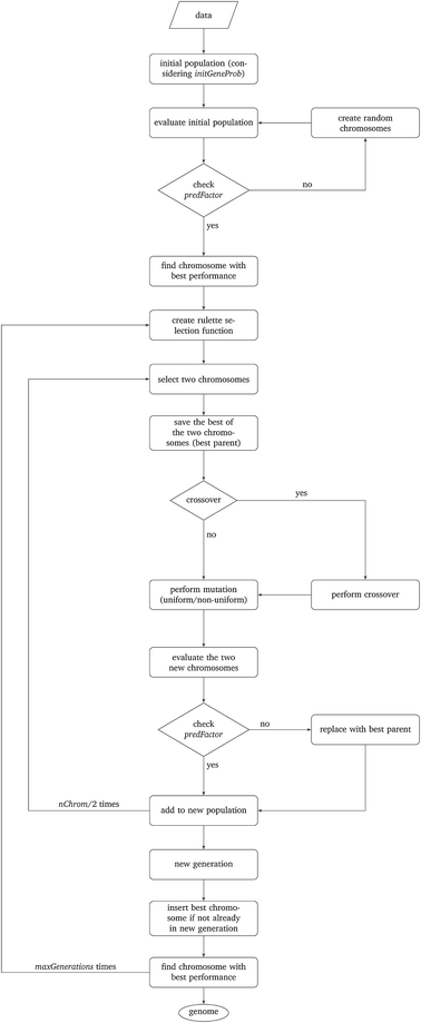
The particular GA developed in this work uses the parameters depicted in Table 2 and is explained next. The algorithm is schematically described in Fig. 1.

Table 2 Initialization parameters of the GA

Initial parameter	Details
nChrom	The size of the population, total number of chromosomes per generation
maxGenerations	The total number of generations
initGeneProb	The probability for a gene to have value 1 initially
crossProb	The probability of crossover
mutProb	The probability for mutation of each gene (uniform)
nonUnf	The mutation probability of the threshold(s) (non-uniform)
thr^GAmin	Lower bound of the threshold(s) value
thr ^GA max	Upper bound of the threshold(s) value
bGA	Freezing parameter
predFactor	Minimum number of samples with produced prediction

---

Fig. 1 Schematic description of the proposed algorithm.

Step I: an initial population of chromosomes is created. The structure of the chromosomes is shown in Table 3. The chromosome is actually a vector, whose length is equal to the number of descriptors L plus the number of similarity criteria used for defining neighbors to a target ENM. The threshold(s) are placed in specific positions in the chromosome representations. This creates hybrid chromosomes containing binary genes for descriptors and real genes for thresholds. The genes related to descriptors correspond to the variables in the construction of the MINLP problem. A value of 1 means that the corresponding descriptor is selected for defining the distance matrix, while a value of 0 means that the descriptor has not been selected. The probability of a binary gene to be coded as 1 is denoted by initGeneProb. The real genes of the chromosomes contain the threshold values corresponding to the similarity criteria and their values are selected randomly from the distance matrices of all samples, considering all variables in each group. In case only one similarity criterion is used, the threshold is placed in the end of the chromosome, whereas if two criteria are used, the two thresholds are placed at the beginning and the end of the chromosome (Table 3).

Table 3 Examples of chromosomes with one and two thresholds

1	0	0	1	0	…	1	1	2.718
2	1.772	1	0	0	…	0	1	1.618

---

Step II: the fitness of each chromosome of the initial population is then calculated as follows:

• The Euclidean distances between all pairs of ENMs are computed using eqn (1) for a single similarity criterion or eqn (10) and (11) for two similarity criteria.

• For each ENM, neighbor ENMs are identified as the ones whose distance from the reference ENM is equal to or lower than the thr value (in the case of two similarity criteria both distances should be equal to or lower than the respective thresholds).

• The algorithm checks if eqn (6) is satisfied, i.e. if ENMs with at least one neighbor are more than predFactor multiplied by the total number of ENMs. If yes, the algorithm proceeds with the next step. If not, the chromosome is rejected, and a new chromosome is generated as described in Step I.

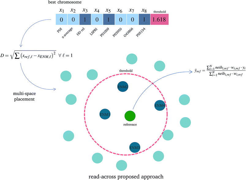
• The read-across predictions are computed using eqn (5) (eqn (21) for two similarity criteria) for ENMs with at least one neighbor. A schematic representation of how the read-across prediction is computed is depicted in Fig. 2.

Fig. 2 A schematic representation of the proposed read-across approach using the selected variables for determining the neighbors in the multi-dimensional space and for obtaining the final read-across prediction. The optimal threshold value defines a circle around a reference ENM (green particle) and ENMs inside the circle are considered as neighbors (blue particles) whereas the remaining ENMs (light blue particles) do not belong to the reference ENM neighborhood and are not involved in the read-across prediction.

• The MSE over all ENMs with at least one neighbor is computed using eqn (22).

• The fitness function value of the chromosome is computed using eqn (23):

• The chromosome with the highest (best) calculated fitness is saved for later analysis.

Step III: a natural selection process takes place and it is iterated maxGenerations times. During each iteration, the following procedure is repeated nChrom/2 times and in total nChrom are selected that form the new generation.

• In order to assure the reproduction of the fittest chromosomes, a “roulette wheel” approach is used.³⁰ The method selects a pair of chromosomes from the previous population, based on randomly generated numbers that indicate the “slots” corresponding to the different chromosomes. The roulette wheel is constructed so that the size of each slot is proportional to the fitness of the corresponding chromosome.³⁰ The roulette is “biased”, thus chromosomes with a reproductive advantage (better fitness scores) have higher probability to be selected. For each pair of selected chromosomes, the one with the highest score is saved as the bestParent for later use.

• The genetic operators of crossover are applied. According to the crossProb value, it is decided if the chromosomes are going to exchange strings of genes or not, in a randomly selected point that indicates the position of crossover.

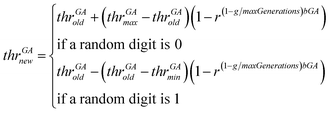
• The genetic operator of mutation is applied. With probability mutProb, binary genes that correspond to a descriptor, invert their value from 0 to 1 and vice versa, while non-uniform mutation is always performed to the threshold values, according to eqn (24).

In eqn (24), thr^GA_old is the old threshold value, thr^GA_new the threshold value that results from the non-uniform mutation, thr^GA_max and thr^GA_min are the upper and the lower bounds of the threshold values, r is a random number between 0 and 1, g is the number of the current generation and bGA is a parameter which determines the degree of dependency on the generation number.

The non-uniform mutation process searches the space uniformly in the first place avoiding stagnation, and as the number of iterations approximates the maximum number of generations, convergence is achieved.²⁹

• The two new chromosomes are evaluated with the procedure described in Step II and in case a chromosome does not meet constraint 6, it is replaced by its bestParent.

In case the best chromosome of the previous generation is not included in the new generation, the algorithm places it in the position of the chromosome with the minimum score, in order to ensure that the chromosome with the best performance will always survive in the evolutionary procedure.

The best chromosome of the last generation is the result of the algorithm. The selected variables and threshold(s)) corresponding to this chromosome will be used subsequently for read-across predictions of unknown ENMs. For evaluating the method, all the training examples are passed through Step II described above to produce the read-across predictions. The correlation coefficient among actual experimental values and read-across predictions (R²) is calculated as follows:

where, y_i and ŷ_i are the experimental and predicted endpoint values over the test set, ȳ and are the averages over the experimental values and the read-across predictions respectively.

4 Validation

An external validation approach is used to test the proposed read-across methodology, by dividing the full dataset into training and test subsets. This data partitioning can be achieved either by applying a random partition or a partition method (e.g. Kennard-Stone).³¹ The training set is used in the GA workflow described above and determines the optimal set of descriptors and threshold(s) values. For the test set, predictions are made using the workflow described in Step II of the algorithm, but now the selected descriptors and the threshold(s) are fixed to their optimal values. Eventually, the read-across predictions are compared with the experimental endpoint values using the q_ext² statistic (eqn (26)).³²where y_i and ŷ_i are the experimental and predicted endpoint values over the test set and ȳ_tr is the averaged value of the endpoint for the training set.

The implementation of the GA algorithm was performed in the Matlab™ programming language. The source code is available at GitHub considering a single threshold (extension to two or more criteria is trivial) (https://github.com/DemetraDanae/optimized-read-across). Minor modifications are needed to make the code compatible with GNU Octave and these are marked as comments.

5 Results and discussion

The proposed read-across method is demonstrated on publicly available data for 84 gold anionic and cationic ENMs, which were included in the publication of Walkey et al.²⁴ For each ENM, the original dataset contains 40 physicochemical descriptors (PDs), 129 protein corona fingerprints (biological descriptors, BDs) and the log2 transformed numerical values for cell association with human A549 cells (in mL/μg (Mg)), where Mg is the total magnesium content to determine the total number of cells, which is considered as the toxicity index to be predicted. We used the filtered dataset derived in the toxFlow web application by Varsou et al.²⁰ after applying the Gene Set Variation Analysis (GSVA)³³ method to BDs, which reduced the biological descriptors to 63 statistically significant proteins. The availability of two different types of descriptors renders this dataset suitable for testing the proposed method with one or two similarity criteria.

The GA method was applied with the operational parameters shown in Table 4. Due to the stochastic nature of the proposed GA strategy, different runs of the algorithm may produce different output results, even if the starting conditions are exactly the same. We selected three levels of the predFactor, and we executed the complete workflow 10 times in the following three variations of the method:

Table 4 Values for the operational parameters of the proposed read-across method

Parameter	Value
nChrom	100
maxGenerations	1000
initGeneProb	0.6
crossProb	0.7
mutProb	0.01
nonUnf	0.1
thr ^GA min	0.1
thr ^GA max	Mean value of the maximum distances between samples
bGA	1
predFactor	0.3–0.6–0.9

---

• Considering a single threshold, corresponding to the full set of descriptors.

• Assuming two different thresholds, one for the group of PDs and one for the group of BDs and obtaining the read-across predictions using the distances between PDs.

• Assuming two different thresholds, one for the group of PDs and one for the group of BDs and obtaining the read-across predictions using the distances between BDs.

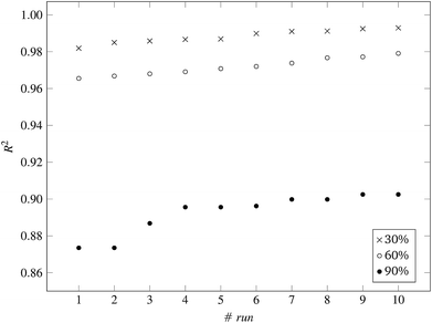
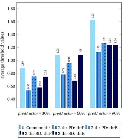
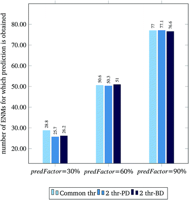
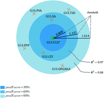
Fig. 3 and 4 present the R² values produced by individual runs of the GA algorithm using one threshold and two thresholds respectively. The results are summarized in Table 5.† As expected, by increasing the value of the predFactor parameter, the optimal threshold values determined by the GA are larger (Fig. 5), which means that read-across predictions are obtained for more ENMs, because there are more ENMs having at least one neighbor (Fig. 6). On the other hand, the accuracy of the read-across predictions measured by the R² statistic is decreased because additional ENMs with higher distances are considered as neighbors to the reference ENM and are involved in the calculation of the read-across prediction. An illustrative example is presented in Fig. 7. By comparing the results between using one or two thresholds, we do not observe significant differences in the number of ENMs with read-across predictions, in the number of selected variables, or in the accuracy of the predictions expressed by R² statistic. The results obtained by using the PD and BD distances for computing the read-across predictions are almost identical.

Fig. 3 R ² values for 10 runs of the GA and three levels of predFactor, using a single threshold.

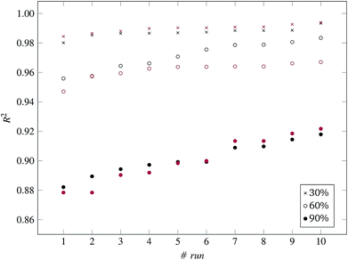Fig. 4 R ² values for 10 runs of the GA and three levels of predFactor, using two thresholds. Black and red markers correspond to predictions using PD and BD distances respectively.

Table 5 Overview of the produced results and statistics from the GA workflow using a single threshold or two thresholds

	Single threshold			Two thresholds
				PD distances			BD distances
	Min	Max	Average	Min	Max	Average	Min	Max	Average
predFactor: 30%
Thresholds	0.5561	1.0134	0.8846	0.4400	0.7579	0.5339	0.3436	0.7440	0.5803
				0.5399	0.8806	0.7499	0.5373	0.8738	0.7455
Selected variables	46	61	53.6	43	56	49.5	48	59	52.1
Predicted samples	26	31	28.8	25	29	25.7	25	28	26.2
R ^2	0.982	0.993	—	0.980	0.993	—	0.984	0.994	—
predFactor: 60%
Thresholds	0.9846	1.1728	1.0843	0.2497	1.0554	0.7806	0.4841	0.8822	0.6844
				0.6766	1.2691	0.9550	0.9780	1.1909	1.0801
Selected variables	46	59	52.3	39	62	50.6	50	62	53.7
Predicted samples	50	53	50.6	50	51	50.3	50	53	51
R ^2	0.966	0.979	—	0.956	0.983	—	0.947	0.967	—
predFactor: 90%
Thresholds	1.5764	1.7488	1.6251	0.9931	1.2318	1.1266	0.9834	1.3869	1.2383
				1.1806	1.3546	1.2671	1.1084	1.4729	1.2399
Selected variables	55	65	60.3	47	64	54.0	48	58	55.2
Predicted samples	76	78	77.0	76	78	77.1	76	79	76.6
R ^2	0.874	0.903	—	0.882	0.918	—	0.878	0.922	—

---

Fig. 5 Average threshold values for different predFactor levels. Five columns are shown at each level. The first column shows the single threshold. The two next columns depict the thresholds corresponding to the groups of PDs and BDs respectively, when distances between PDs are used for the read-across predictions. The last two columns present the two thresholds again, when read-across predictions are performed using the distances between BDs.

Fig. 6 Average number of ENMs for which prediction is obtained per different predFactor levels.

Fig. 7 An example of the effect of the predFactor on the threshold, the number of neighbors and the predictive accuracy. The reference ENM is depicted with green color and the orange ENMs are candidate neighbors. By increasing the predFactor value, the threshold is increased, more ENMs with higher distances to the reference ENM are considered as neighbors and less accurate predictions are obtained. The single threshold variant is considered and a 2D projection of the multi-dimensional space is presented.

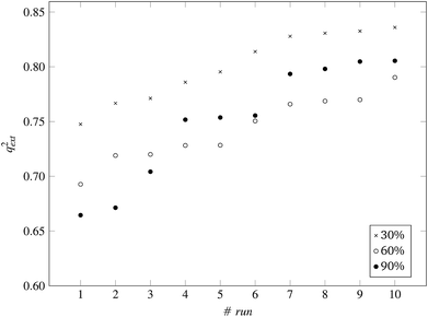Fig. 8 q _ext ² values for 10 runs of the GA and three levels of predFactor, using a single threshold.

The prediction accuracy of the proposed method, using the 60% predFactor level, is similar to the application of toxFlow²⁰ on the same dataset, in terms of the R² statistic (toxFlow produced a 0.973R² value). However, the method proposed in this work was able to produce read-across predictions for significantly more ENMs (average 50 to 51 ENMs compared to 21 ENMs in toxFlow).

For the 60% predFactor level, we also measured the frequency of appearance of the different descriptors in the selected sets of descriptors. It is clear that there exist descriptors which are selected in most runs, whereas some other descriptors are chosen very rarely. The descriptors appearing in more than 70% of the runs are considered as the most significant descriptors. The most frequently selected PDs and BDs are presented in Fig. 10 and 11 respectively.

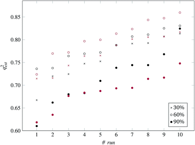Fig. 9 q _ext ² values for 10 runs of the GA and three levels of predFactor, using two thresholds. Black and red markers correspond to predictions using PD and BD distances respectively.

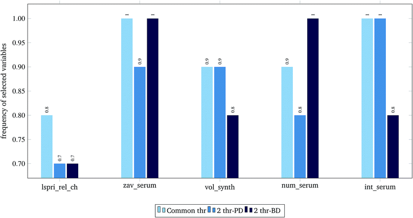Fig. 10 Selected physicochemical variables in frequency greater than 0.7, at predFactor ratio equal to 0.6.

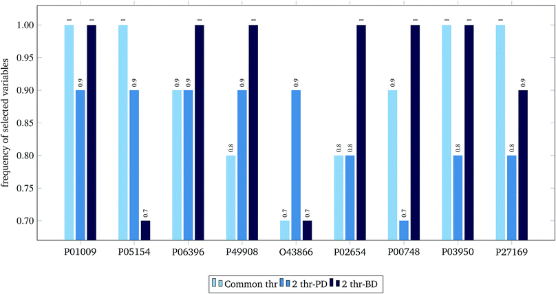Fig. 11 Selected biological variables in frequency greater than 0.7, at predFactor ratio equal to 0.6.

The presented descriptors in Fig. 10 are extracted from ENM characterization assays²⁴ and are further described next:

• lspri_rel_ch: ({LSPRi after serum exposure} − {LSPRi after synthesis})/{LSPRi after synthesis}

• zav_serum: Z-average hydrodynamic diameter (HD) after serum exposure.

• vol_synth: volume mean HD after synthesis.

• num_serum: number mean HD after serum exposure.

• int_serum: intensity mean HD after serum exposure.

The localized surface plasmon resonance index (LSPRi) for each sample is computed from collected absorbance spectra, and is an empirical measure of the local dielectric environment surrounding plasmonic ENMs. The rest of the presented descriptors are measured by Dynamic Light Scattering (DLS) characterization, using the available commercial software of the instrument (ZetaSizer Nano ZS, Malvern Instruments).²⁴ The HD parameter expresses “the size of a hypothetical hard sphere that diffuses in the same fashion as that of the particle being measured”.³⁴ The HD diameter is an important factor for ENM characterization as it helps understand migration of ENMs into the (biological) media. Within a liquid (biological) medium, an electric dipole layer (in our case the protein corona) is formed around the dispersed ENM due to the surrounding macro-molecules and influences its Brownian diffusion into the medium.^35–38 Therefore, the HD diameter encloses information of the ENM core along with any attached coating and formed solvent layer, a type of information that is based on resembled exposure conditions and cannot be estimated by other methods (e.g. size measured by TEM microscopy).

The hypergeometric test was applied to the most frequently selected BDs shown in Fig. 11, considering all genes (ENTREZ IDs) included in the molecular function category of the gene ontology (GO) at the time of writing this paper (45 099).²² The most statistically significant GO terms (p-value < 0.001) are depicted in Table 6.

Table 6 Significant GO terms containing the proteins selected by at least seven GA runs in all three variations. The size of the gene sets is placed in parenthesis next to their GO term name

GO term name	GO term ID	ENTREZ IDs	UNIPROT	p-value
Acrosin binding (4)	GO: 0032190	5104	P05154	0.00080
Acyl-L-homoserine-lactone lactonohydrolase activity (3)	GO: 0102007	5444	P27169	0.00060
Aryldialkylphosphatase activity (3)	GO: 0004063	5444	P27169	0.00060
Heparin binding (220)	GO: 0008201	283	P03950	0.00082
		5104	P05154
Phosphatidylcholine binding (24)	GO: 0031210	341	P02654	0.00001
		5104	P05154
Phosphatidylcholine-sterol O-acyltransferase activator activity (5)	GO: 0060228	341	P02654	0.00100
Protease binding (143)	GO: 0002020	5265	P01009	0.00035
		5104	P05154
Serine-type endopeptidase inhibitor activity (202)	GO: 0004867	5265	P01009	0.00070
		5104	P05154

---

Finally, the full dataset was divided into training and test sets in a ratio of 66 : 33 (55 training and 29 test ENMs) using the Kennard and Stones method.³⁹ We applied all three variations of the method described in the beginning of this section to the training data only. The selected variables and optimal threshold value(s) obtained by the solution of the optimisation problems were applied for computing read-across predictions for the test ENMs. The results are summarized in Table 7† and in Fig. 8 and 9 for the single threshold and the two-threshold cases respectively. We observe that the predFactor does not play a major role, obviously because the Kennard-Stone algorithm forces the validation samples to be within the space defined by the training data. Even with the 30% predFactor level, read-across predictions were obtained for most ENMs in the test set. The best results in terms of the q_ext² statistic were produced with the 60% predFactor level using two thresholds and the BD distances for calculating the read-across predictions. The prediction accuracy drops down significantly when applying the 90% predFactor level, because in this case, as indicated before (Fig. 5–7), the optimal threshold values are increased and the algorithm considers as neighbors source ENMs with higher distances (not very similar) to the target ENM.

Table 7 Overview of the GA validation results and statistics using a single threshold or two thresholds

	Single threshold			Two thresholds
				PD distances			BD distances
	Min	Max	Average	Min	Max	Average	Min	Max	Average
predFactor: 30%
Thresholds	1.0680	1.4009	1.2682	0.3336	0.7728	0.6158	0.4084	0.7793	0.5826
				1.0302	1.8066	1.3124	0.9279	1.8881	1.3770
Selected variables	43	62	56.4	44	61	52.8	43	60	52.1
Predicted samples	27	29	28.0	22	29	26.2	24	28	26.3
q ext ^2	0.748	0.836	—	0.667	0.813	—	0.698	0.817	—
predFactor: 60%
Thresholds	1.3923	1.7148	1.4889	0.6779	1.3573	0.9772	0.8416	1.3832	1.0055
				1.1047	1.5270	1.3093	1.1309	1.4679	1.2805
Selected variables	50	57	55	47	62	55.6	48	62	54.6
Predicted samples	29	29	29	28	29	28.7	27	29	28.4
q ext ^2	0.693	0.790	—	0.736	0.831	—	0.724	0.860	—
predFactor: 90%
Thresholds	1.6594	1.9079	1.7494	1.1468	1.9579	1.4414	1.1214	1.5443	1.3407
				1.0865	1.7443	1.3872	1.1924	1.5521	1.3985
Selected variables	52	63	56.8	45	64	55.0	50	67	58.5
Predicted samples	29	29	29.0	29	29	29.0	29	29	29
q ext ^2	0.664	0.806	—	0.610	0.824	—	0.618	0.748	—

---

6 Conclusions

In this work, a novel read-across method to predict toxicity related endpoints of ENMs has been developed. The method offers two important advantages compared to standard read-across approaches. First, it considers explicitly the multi-perspective characterisation of ENMs, by defining multiple thresholds relative to different similarity criteria and ensuring that two ENMs are considered as neighbors only if they satisfy all similarity requirements. Secondly, it performs an automatic extensive search over the solution space in order to find the read-across hypothesis that produces the best possible results in terms of prediction accuracy and number of ENMs for which predictions are obtained. Thus, it overcomes a main drawback of existing time approaches, which are based on manually trying different read-across hypotheses in an iterative, inefficient and time-consuming trial and error fashion. The main outcomes of the method are: a reduced set of significant descriptors and a single or multiple threshold values which rigorously define the boundaries around a query ENM, where neighboring ENMs are located. The presented workflow is rather flexible and can be extended or modified in the future to accommodate additional similarity criteria, alternative prediction functions (other than the weighted average) and solve classification read-across problems where the end-point is a discrete rather than a continuous variable.

Conflicts of interest

There are no conflicts to declare.

Abbreviations

BD	Biological descriptor
CTD	Comparative toxicogenomics database
DLS	Dynamic light scattering
ECHA	European Chemicals Agency
(E)NM	(Engineered) nanomaterial
GA	Genetic algorithm
GSVA	Gene set variation analysis
HD	Hydrodynamic diameter
LSPRi	Localized surface plasmon resonance index
MSE	Mean squared error
MWCNT	Multi-walled carbon nanotube
NP	Nanoparticle
OECD	Organization for Economic Co-operation and Development
OF	Objective function
PCA	Principal components analysis
PCF	Protein corona fingerprints
PD	Physicochemical descriptor
QNAR	Quantitative nanostructure–activity relationship (modeling)
QSAR	Quantitative structure–activity relationship (modeling)
QM	Quantum mechanical
SVM	Support vector machine

Acknowledgements

D-DV acknowledges funding from the Onassis Foundation for her PhD studies. AA, GM and HS acknowledge support by the NanoCommons project, which has received funding from the European Union Horizon 2020 Programme (H2020) under grant agreement no. 731032.

References

1. M. Fojtü, W. Z. Teo and M. Pumera, Environ. Sci.: Nano, 2017, 4, 1617–1633.
2. I. L. Gunsolus and C. L. Haynes, Anal. Chem., 2015, 88, 451–479.
3. B. He, Y. Shi, Y. Liang, A. Yang, Z. Fan, L. Yuan, X. Zou, X. Chang, H. Zhang and X. Wang, Nat. Commun., 2018, 9, 2393.
4. A. Gajewicz, B. Rasulev, T. C. Dinadayalane, P. Urbaszek, T. Puzyn, D. Leszczynska and J. Leszczynski, Adv. Drug Deliv. Rev., 2012, 64, 1663–1693.
5. A. Gajewicz, K. Jagiello, M. T. Cronin, J. Leszczynski and T. Puzyn, Environ. Sci.: Nano, 2017, 4, 346–358.
6. J. H. Arts, M. Hadi, M.-A. Irfan, A. M. Keene, R. Kreiling, D. Lyon, M. Maier, K. Michel, T. Petry and U. G. Sauer, Regul. Toxicol. Pharmacol., 2015, 71, S1–S27.
7. EU Directive, Official Journal of the European Union, 2010, 276, 33–74.
8. D. A. Winkler, E. Mombelli, A. Pietroiusti, L. Tran, A. Worth, B. Fadeel and M. J. McCall, Toxicology, 2013, 313, 15–23.
9. J. J. Villaverde, B. Sevilla-Morán, C. López-Goti, J. L. Alonso-Prados and P. Sandín-España, Sci. Total Environ., 2018, 634, 1530–1539.
10. L. Lamon, D. Asturiol, A. Vilchez, R. Ruperez-Illescas, J. Cabellos, A. Richarz and A. Worth, Comput. Toxicol., 2018, 15(1), 37.
11. EU Science Hub, Review of Computational Models for the Safety Assessment of Nanomaterials, 2017, https://ec.europa.eu/jrc/en/science-update/review-computational-models-safety-assessment-nanomaterials.
12. A. Gajewicz, Environ. Sci.: Nano, 2017, 4, 1389–1403.
13. ECHA, Read-across Assessment Framework, 2017, https://echa.europa.eu/documents/10162/13628/raaf_en.pdf.
14. T. Schultz, P. Amcoff, E. Berggren, F. Gautier, M. Klaric, D. Knight, C. Mahony, M. Schwarz, A. White and M. Cronin, Regul. Toxicol. Pharmacol., 2015, 72, 586–601.
15. A. G. Oomen, E. A. Bleeker, P. M. Bos, F. van Broekhuizen, S. Gottardo, M. Groenewold, D. Hristozov, K. Hund-Rinke, M.-A. Irfan and A. Marcomini, Int. Res. J. Public Environ. Health, 2015, 12, 13415–13434.
16. L. Lamon, D. Asturiol, A. Richarz, E. Joossens, R. Graepel, K. Aschberger and A. Worth, Part. Fibre Toxicol., 2018, 15, 37.
17. A. Mech, K. Rasmussen, P. Jantunen, L. Aicher, M. Alessandrelli, U. Bernauer, E. Bleeker, J. Bouillard, P. Di Prospero Fanghella and R. Draisci, Nanotoxicology, 2019, 13(1), 119–141.
18. A. Gajewicz, M. T. Cronin, B. Rasulev, J. Leszczynski and T. Puzyn, Nanotechnology, 2014, 26, 015701.
19. C. Helma, M. Rautenberg and D. Gebele, Front. Pharmacol., 2017, 8, 377.
20. D.-D. Varsou, G. Tsiliki, P. Nymark, P. Kohonen, R. Grafstrom and H. Sarimveis, J. Chem. Inf. Model., 2017, 58, 543–549.
21. C. M. Sayes, P. A. Smith and I. V. Ivanov, Int. J. Nanomed., 2013, 8, 45.
22. North Carolina State University, Comparative Toxicogenomics Database, 2019, http://ctdbase.org/.
23. T. Puzyn, B. Rasulev, A. Gajewicz, X. Hu, T. P. Dasari, A. Michalkova, H.-M. Hwang, A. Toropov, D. Leszczynska and J. Leszczynski, Nat. Nanotechnol., 2011, 6, 175.
24. C. D. Walkey, J. B. Olsen, F. Song, R. Liu, H. Guo, D. W. H. Olsen, Y. Cohen, A. Emili and W. C. Chan, ACS Nano, 2014, 8, 2439–2455.
25. ECHA, Guidance on Information Requirements and Chemical Safety Assessment, Appendix R.6-1 for Nanomaterials Applicable to the Guidance on QSARs and Grouping of Chemicals, May 2017, https://echa.europa.eu/documents/10162/23036412/appendix_r6_nanomaterials_en.pdf.
26. K. Aschberger, D. Asturiol, L. Lamon, A. Richarz, K. Gerloff and A. Worth, Comput. Toxicol., 2019, 9, 22–35.
27. Organization for Economic Cooperation & Development, Case Study on Grouping and Read-Across for Nanomaterials Genotoxicity of Nano-TIO₂, September 2018, http://www.oecd.org/officialdocuments/publicdisplaydocumentpdf/?cote=ENV/JM/MONO(2018)28%26docLanguage=En.
28. A. R. Leach and V. J. Gillet, An Introduction to Chemoinformatics, Springer Science & Business Media, 2007.
29. A. Alexandridis, P. Patrinos, H. Sarimveis and G. Tsekouras, Chemometr. Intell. Lab. Syst., 2005, 75, 149–162.
30. G. A. Chourdakis, BS thesis, National Technical University of Athens, School of Chemical Engineering, Athens, Greece, 2014.
31. A. Tropsha, Mol. Inf., 2010, 29, 476–488.
32. A. Tropsha, P. Gramatica and V. K. Gombar, QSAR Comb. Sci., 2003, 22, 69–77.
33. S. Hänzelmann, R. Castelo and J. Guinney, BMC Bioinf., 2013, 14, 7.
34. Worldwide, Malvern Instruments, Inform white paper, Dynamic light scattering, Common terms defined, Malwern Instruments Limited, 2011, vol. 2011, pp. 1–6.
35. J. Lim, S. P. Yeap, H. X. Che and S. C. Low, Nanoscale Res. Lett., 2013, 8, 381.
36. J. Stetefeld, S. A. McKenna and T. R. Patel, Biophys. Rev., 2016, 8, 409–427.
37. A. Dhawan and V. Sharma, Anal. Bioanal. Chem., 2010, 398, 589–605.
38. G. V. Lowry, R. J. Hill, S. Harper, A. F. Rawle, C. O. Hendren, F. Klaessig, U. Nobbmann, P. Sayre and J. Rumble, Environ. Sci.: Nano, 2016, 3, 953–965.
39. M. Daszykowski, B. Walczak and D. Massart, Anal. Chim. Acta, 2002, 468, 91–103.

---

Footnote

† Summarized results of 10 runs of the GA algorithm are depicted.

---