Predicting aggregation energy for single atom bimetallic catalysts on clean and O* adsorbed surfaces through machine learning models†
Zhuole
Lu
a,
Shwetank
Yadav
a and
Chandra Veer
Singh
 *ab
*ab
aDepartment of Materials Science and Engineering, University of Toronto, 184 College St, Toronto, ON M5S 3E4, Canada. E-mail: chandraveer.singh@utoronto.ca
bDepartment of Mechanical and Industrial Engineering, University of Toronto, Canada
First published on 18th November 2019
Abstract
Single atom catalysts have received increased attention due to their unprecedented high metal dispersion. Recent progress in machine learning (ML) has significantly aided in the rational design of such heterogeneous catalysts, often dedicated to ML prediction of adsorption properties. A common shortfall, however, is the neglect of the thermodynamic stability of the assumed site and adsorbate-induced structural changes. Here, we developed ML models to predict the thermodynamic stability of a single-atom and related site of 38 different elements alloyed with Cu, trained with DFT calculations. To account for adsorbate-induced effects, we placed a monoatomic oxygen adsorbate in the vicinity of the dopant site. A Gaussian process regression (GPR) model performed best with a mean absolute error (MAE) of less than 0.08 eV for aggregation energy. The same performance was achieved with an even smaller training dataset using an active learning algorithm, producing a one-third time saving. Similarly, our ML prediction of O* adsorption energy gave a MAE of 0.08 eV. Furthermore, the ML model is extendable to different substrates (in addition to Cu), different adsorbates (in addition to O*), and larger cluster sizes (greater than trimer), demonstrating the potential of addressing large number of degrees of freedom and orders of magnitude time saving.
1. Introduction
Heterogeneous catalysts play arguably the most important role in the modern chemical industry, as they reduce the kinetic barriers for numerous chemical processes, thereby increasing production rates and reducing energy consumption.1 The pressing issues of global warming, energy resource depletion and environmental pollution call attention to the need for sustainable development. As a sector that accounts for nearly 20% of all energy consumption in OECD countries,2 the chemical industry has been heavily invested in designing more efficient catalysts as well as making green chemical processes more viable.Bimetallic catalysts can present increased activity, selectivity and stability in comparison to monometallic catalysts.3 They offer a vast chemical space through combining different metals and mixing ratios. There are a wide variety of bimetallic structures, including surface alloys,4 near-surface alloys5 and core–shell nanoparticles,6 each with their own unique catalytic properties. Single atom catalysts (SACs), consisting of single active metal atoms dispersed on a support, in particular have received increasing attention recently as they can overcome one of the challenges of heterogeneous catalysts, namely a low active metal utilization due to aggregation of this active metal's atoms in clusters with a low exposed surface to volume ratio. SACs on the other hand can maximize this active surface area while remaining stable in some cases. When the support in a SAC is also a metal, it can be referred to as a single atom alloy (SAA). SAAs can have strong electronic interaction and synergistic effects between the metals as well geometric and strain effects. Hence, SAAs can be more stable than the more common oxide-supported or carbon-supported SACs.7
Computational modeling tools, predominantly density functional theory (DFT) calculations, provide a more convenient and less expensive method of exploring the available catalyst chemical space compared to experiments. They have been leading the discovery of new bimetallic catalysts8,9 as well as novel scientific insights.10 While DFT calculations can provide nano-scale insights in cases where experimental studies are of limited help, they can still be computationally expensive when comparing large numbers of systems. Machine learning (ML) methods can help reduce the number of DFT simulations and have demonstrated reasonable accuracy with lower computing time when applied to heterogeneous catalysis and surface science.11
There have been a number of studies utilizing ML to predict adsorption energies on bimetallic surfaces;12–14 however, few studies have addressed the thermodynamic stability of the underlying bimetallic site assumed in these ML works. Furthermore, the bimetallic surfaces used in predicting the adsorption energies may not be the most favorable one upon adsorption of reactants during reaction. Adsorbate-induced structural changes are well-known, observed experimentally (segregation15–17 and aggregation18,19) and studied theoretically.20–22 Menning et al. systematically studied trends in adsorbate-induced segregation and correlated the tendency for surface segregation with d-band center;21 however, obtaining the d-band center itself still requires costly DFT calculations. There remains a need for direct prediction of adsorbate-induced aggregation using simple, readily available descriptors.
In this work, we build ML models to predict the DFT-calculated ground state energies of aggregation for SAAs and larger two-atom (dimer) and three-atom (trimer) clusters which can act as bimetallic sites for reactions. We test 38 active metals with a Cu substrate. The developed ML models use the following readily accessible elemental properties: atomic number, group number, period number, atomic radius, and electronegativity (Pauling scale). Furthermore, we ensure the model can also predict the effect of an adsorbed O* atom on the site, a common intermediate in several important reaction systems, on these aggregation energies. In modelling these properties, we note a strong effect of training/testing data split, and we selectively use Gaussian process regression models to illustrate these effects. Finally, we demonstrate an active learning scheme that can automatically select training points, resulting in significant time saving.
The ML models developed in this work is, moreover, capable of sampling the vast bimetallic catalyst space spanned by different substrates, different adsorbates, and larger cluster size, in addition to different secondary metals (dilute metals), thereby bringing orders of magnitude reduction in computational time required for catalyst screening. Furthermore, minimal modification is required to extend the model to the aforementioned additional degrees of freedom. We believe this highly transferable ML platform will significantly contribute to the progress toward rational catalyst design of SAA's.
2. Methodology
2.1 Density functional theory (DFT) calculations
All calculations were carried out using the plane wave based DFT VASP software package. Simulations were done through projector augmented wavefunctions (PAW)23 with the Perdew–Burke–Ernzerhof (PBE) exchange functional.24 The energy wavefunction cutoff was set at 400 eV and reciprocal space was sampled using a 5 × 5 × 1 Monkhorst–Pack k-point grid. Self-consistent field calculations were set to stop when energy change was smaller than 0.0001 eV. The systems were relaxed until the forces acting on each atom were less than 0.05 eV Å−1.2.2 Surface models
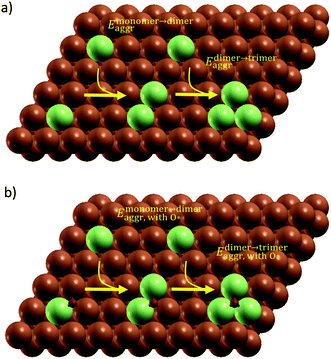
All simulation structures were created by starting with a Cu four-layer (3 × 3) slab model cleaved along the (111) plane. We compared the (3 × 3) supercell with (4 × 4) supercell and found that the (3 × 3) supercell is sufficiently large to avoid periodic interactions (sections 1 and 2 in ESI†). Each supercell had 15 Å of vacuum separation in the surface normal direction. In order to create a SAA surface, one Cu atom in the top layer was replaced with a dopant metal atom (M atom), forming a monomer (Fig. 1). A dimer site was created to represent the first step of aggregation, where a neighboring Cu of the single M atom was also replaced with M. Further aggregation for trimer formation was created by replacing a Cu atom neighboring to the two M atoms of the dimer site with an M atom, forming a triangular trimer site. In order to calculate adsorbate-induced aggregation, an O* adsorbate was placed at a position corresponding to the center of the triangular M trimer.Reactant-induced ripening has been well studied on oxide-supported metal catalysts (TiO2-supported Rh (ref. 25) and CeO2-supported Pt,26 both under CO influence) on the basis of thermodynamics, which provide useful strategies for stabilizing metal single atoms. Here, we studied the stability of single atom alloys and determined the energies required to aggregate from monomer to dimer, and from dimer to trimer, with and without adsorbate (O*) influence. The aggregation energy (Eaggr), the energy required to add another dopant atom to an existing dopant site (of one or more atoms), is defined as:
| Emonomer→dimeraggr = E(Cu–M–M) + E(Cu–Cu–Cu) − 2E(Cu–Cu–M) | (1) |
| Edimer→trimeraggr = E(M–M–M) + E(Cu–Cu–Cu) − E(Cu–M–M) − E(Cu–Cu–M) | (2) |
| Emonomer→dimeraggr,with O* = EO*(Cu–M–M) + E(Cu–Cu–Cu) − EO*(Cu–Cu–M) − E(Cu–Cu–M) | (3) |
| Edimer→trimeraggr,with O* = EO*(M–M–M) + E(Cu–Cu–Cu) − EO*(Cu–M–M) − E(Cu–Cu–M) | (4) |
| Emonomer→trimeraggr = Emonomer→dimeraggr + Edimer→trimeraggr |
Adsorption energies of O* were determined relative to the gas-phase O2 molecule according to the following equation:
| Eads,O* = EO*(surface) − E(surface) − 1/2EO2 |
3. Results and discussion
3.1 Trends in aggregation energies
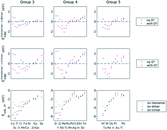
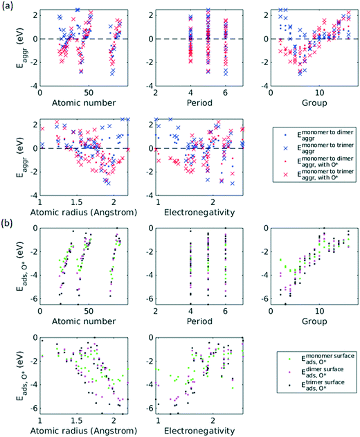
A total number of 38 metals were included for study, consisting of metal elements from periods 4, 5, and 6. Six features were selected to be fed into the ML models for adsorption energy predictions, the first five of which were the following elemental properties: atomic number, group numbers, period numbers, atomic radius (empirically measured),30 and electronegativity (Pauling scale).31 Data for these five features are readily available from common data sources and require no further calculations. These five features were chosen based on previous works on feature engineering,12,32 from which we identified the most important ones. The sixth feature for predicting Eads was categorical and indicated whether the adsorption site in the initial state was a monomer, dimer or trimer. For Eaggr prediction, the same features were included along with an additional categorical feature indicating whether the O* adsorbate was present, giving a total of seven features. Details regarding implementation of ML algorithms and cross validation are given in the ESI.†The results for Eaggr are shown in Fig. 3. Periodic trends are clearly discernible in Eaggr, characterized by energy minima at group numbers of around 3 to 5. This periodic trend is more pronounced in period 4 and 5 elements compared to period 3, with a wider energy range. The signs of dimer and trimer formation energies are always consistent, indicating that favorable dimer formation can always be followed by trimer formation. The positive Eaggr (single-atom alloy is favored) of Pt and Pd were previously confirmed experimentally using scanning tunneling microscope (STM) techniques.33,34 On the other hand, the negative Eaggr of Co and Fe indicate that aggregation is favored for these metals on Cu substrate, which is indeed frequently observed during thin film growth experiments on Cu(111) substrate.35
The inclusion of O* adsorbate brings some period 3 elements' Eaggr down by a significant extent, and can destabilize single-atom alloys for lower group numbers in periods 3 and 4 that would otherwise be stable for the clean surface. The extent of O*-induced downward shifts generally become smaller as group number increases, which follows the same trend of electronegativity increase, suggesting that O*-induced aggregation is correlated with electronegativity of the dilute metal (Fig. 4a). On the other hand, for some elements, Eaggr is increased by introducing O* adsorbate. For instance, the Emonomer→trimeraggr,with O* on Pd is increased by more than 1 eV compared to surface without O*, which is consistent with literature reported increase in degree of alloying in the surface region of a CuPd alloy sample.36
3.2 Trends in O* adsorption energies
Prediction of adsorption energies has been successfully developed using the d-band theory10 and its derived frameworks,37–39 although prediction on alloys has been shown to be more complicated, requiring not only the d-band center but characteristics of d-band shape.14,40 Here, we attempt to predict Eads,O* based solely on basic elemental features, avoiding expensive d-band computation. For Eads,O*, Fig. 3, periodic trends are similarly observed, and a number of patterns resemble those of Eaggr. Adsorption energies generally increase (corresponding to less stable or favorable adsorption) with increasing group number. Strong O* adsorption is in general also coupled with favorable formation of dimers and trimers (which also occurs for lower group numbers). This is similar to the synergistic effects between strong adsorbate binding and surface segregation.29 For most metals, trimers adsorb O* more strongly than dimers and monomers, particularly toward the region of Eads,O* minima.3.3 ML model design
Feature selection is the process of identifying the most relevant descriptors for representing the input to ML models. Criteria for feature selection usually involve two aspects: (1) reduction of irrelevance and (2) reduction of redundancy. Much work has been dedicated to feature engineering for modelling heterogeneous catalysis, and those features generally fall into three categories: element-related features (e.g. electronegativity, atomic radius, ionization energy, electron affinity),12 adsorbate-related features (e.g. chemical bonds, molecular fragments, and size of molecule),41 and structure-related features (e.g. coordination number and its generalized form).42 Our data encompass all three aforementioned categories, spanning across different dilute metal identities (element-related features), absence/presence of O* adsorbate (adsorbate-related features), and number of dilute metal atoms (structure-related features).Based on the literature, we initially included 10 features: atomic number (Z), atomic weight (Ar), period number (P), group number (G), atomic radius (R), electronegativity (EN), ionization energy, electron affinity, number of dilute metal atoms, and binary input for absence/presence of O*. Since the Cu substrate remains the same, substrate is not included in the feature vector except in the transferability analysis in section 3.6. An initial feature selection experiment, using exhaustive feature search with a squared exponential kernel-based GPR model, revealed that the element dimension was best described by Z, P, G, R, and EN. In order to compare the relative importance of each feature, we performed sensitivity analysis on the inputs using the perturbation method (section 4 in ESI†).14,43 Results indicated that R, EN, and G play a more important role (with correlations over 0.7), while Z and P contributes less to the prediction (Fig. 5). We note that other sensitivity methods, most notably the Sobol method,44,45 are capable of capture higher order feature sensitivity and could provide more insights, but they are only applicable to independent inputs whereas our features are interdependent (e.g. EN and G).
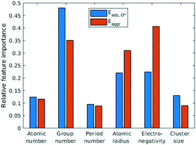 | ||
| Fig. 5 Quantification of feature importance in ML prediction of adsorption and aggregation energies using the perturbation sensitivity analysis. | ||
The results from sec. 3.1 showed that, while periodic trends are clearly present in Eaggr and adsorption energy, they show complex patterns, including multiple local minima, changing monotonicity, and lack of linearity. These complex patterns present significant challenges for applying traditional parametric models, such as stepwise linear fitting40 and quadratic fitting,21 all of which presume certain parameterized models can fit the data. Accordingly, we resorted to non-parametric models, which do not presume any explicit relationship between input and output. Non-parametric models make predictions solely from the training data, (for example, by comparing with the most similar instances in the training set, i.e. k nearest neighbor algorithm) and are particularly robust for handling complex data.46
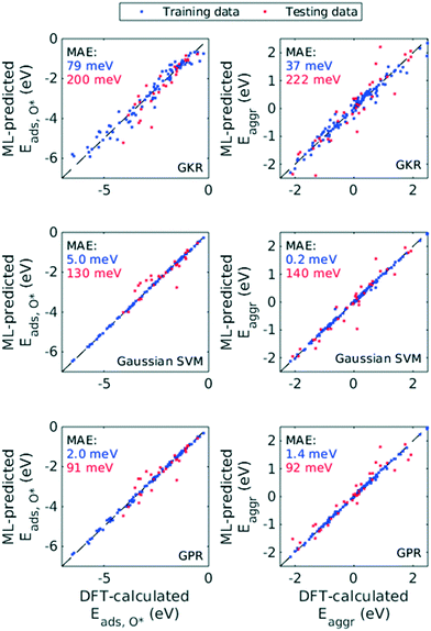
Hence, we chose the three most popular non-parametric models: Gaussian kernel regression (GKR), Gaussian kernel-based support vector machine (SVM) and Gaussian process regression (GPR). Performance of these ML models was quantified with RMSE, MAE and R2, both for Eaggr and Eads,O* (Table 1). All ML models were trained assuming all features are numerical variables. All three ML models made reasonably accurate predictions, with RMSE less than 0.5 eV and MAE less than 0.3 eV for the testing set (Fig. 6). For both Eaggr and Eads,O*, GPR gave the best performance, followed by SVM and lastly GKR. The best performer, GPR, yielded an RMSE of 0.30 eV, a MAE of 0.09 eV and an R2 greater than 0.9 on both aggregation and adsorption energy testing sets. All ML models were possibly overfit, indicated by the good performance on the training sets and lower on the testing sets. Among them, SVM was most severely overfit, with nearly perfect fitting on the training set but limited generalizability to the testing set.
| ML model | Training set (75%) | Testing set (25%) | ||||
|---|---|---|---|---|---|---|
| RMSE (meV) | MAE (meV) | R 2 | RMSE (meV) | MAE (meV) | R 2 | |
| Aggregation energy (Eaggr) | ||||||
| Gaussian kernel regression (GKR) | 190 ± 20 | 37 ± 8 | 0.97 ± 0.01 | 464 ± 87 | 222 ± 87 | 0.80 ± 0.08 |
| Gaussian kernel supported vector machine (SVM) | 11 ± 7 | 0.2 ± 0.2 | 1.00 ± 0.00 | 369 ± 66 | 140 ± 52 | 0.87 ± 0.05 |
| Gaussian process regression (GPR) | 38 ± 4 | 1.4 ± 0.3 | 1.00 ± 0.00 | 298 ± 56 | 92 ± 63 | 0.91 ± 0.03 |
| Adsorption energy of O* (Eads,O*) | ||||||
| Gaussian kernel regression (GKR) | 281 ± 16 | 79 ± 9 | 0.96 ± 0.00 | 438 ± 86 | 200 ± 81 | 0.90 ± 0.04 |
| Gaussian kernel supported vector machine (SVM) | 70 ± 1 | 50 ± 0.2 | 1.00 ± 0.00 | 350 ± 87 | 130 ± 67 | 0.94 ± 0.03 |
| Gaussian process regression (GPR) | 47 ± 12 | 2 ± 1 | 1.00 ± 0.00 | 296 ± 60 | 91 ± 38 | 0.95 ± 0.02 |
We chose GPR as our primary ML model for the rest of the discussion. We based this decision on two facts: (1) its exceedingly good performance as indicated by RMSE, MAE and R2, (2) likely existence of Gaussian-distributed noise in DFT calculations,47 and (3) its ability to give uncertainty on each prediction it makes. The last advantage arises from GPR's theoretical framework, Bayesian inference, which enables calculation of posterior probability distribution given prior probability and appropriate likelihood function. We note that non-Bayesian methods, such as GKR and SVM explored in this work, can also quantify uncertainties indirectly, through Monte-Carlo simulations and perturbation models for example.48 However, the Bayesian nature of GPR method allows more efficient and more interpretable uncertainty analysis.
Our results demonstrated that the GPR model can accurately predict for O*-induced changes, which is important in rational catalyst design under realistic reaction conditions. Following the same random leave-25%-out procedure (repeated 100 times) for splitting training and testing datasets, we computed performance indicators separately for Eaggr and Eaggr,withO* (Table 2). Similar performance was achieved for both data categories, with prediction on O*-covered sites slightly more accurate. Moreover, the GPR model correctly predicted the sign of energy change for 87% of the testing data points. We note that in quantifying these performance metrics, we only included data points whose clean-surface energy and O*-induced energy were both in the testing set. The ability of the GPR model to handle subtle aspects of the data such as O*-induced changes demonstrates the robustness of GPR model.
| Data category | Testing set (25%) | ||
|---|---|---|---|
| RMSE (meV) | MAE (meV) | R 2 | |
| Aggregation energies on clean surfaces (Eaggr) | 309 ± 82 | 102 ± 55 | 0.88 ± 0.07 |
| Aggregation energies with O* adsorbate (Eaggr,with O*) | 276 ± 66 | 80 ± 40 | 0.92 ± 0.03 |
3.4 Uncertainty quantification with GPR
Increasing training set ratio improves a ML model's understanding of the data and, assuming no overfitting exists, lowers prediction error in the testing set. Knowing GPR's ability to provide uncertainty estimation (section 3.2.2), we demonstrated that the GPR model can give uncertainty that is in line with the real error (measured with MAE, Table 3) and in general agreement with the aforementioned relationship between training set ratio and predictive error. When increasing training set ratio from 75% to 90%, the mean value of σ stayed unchanged (for both Eaggr and Eads,O*), suggesting that the amount of training data was sufficient for the GPR model and was confirmed with nearly unchanged MAEs. The percentage of data falling within ±2σ of posterior was around 85% to 90%, indicating that the majority of data could be predicted with confidence. Note that the ±2σ range corresponds to a 95% confidence interval, and our lower-than-expected fractions of data falling within ±2σ suggests that our data might contain non-Gaussian noise, our kernel is not a perfect similarity measure, and/or some features are missing.| Training/testing dataset ratio | Testing set | ||
|---|---|---|---|
| MAE (meV) | Mean value of σ (meV) | Fraction of data falling within ±2σ | |
| Adsorption energy of O* (Eads,O*) | |||
| 50%/50% | 138 ± 40 | 298 ± 33 | 0.90 ± 0.05 |
| 75%/25% | 91 ± 38 | 213 ± 19 | 0.84 ± 0.08 |
| 90%/10% | 64 ± 41 | 212 ± 32 | 0.90 ± 0.08 |
| Aggregation energy (Eaggr) | |||
| 50%/50% | 202 ± 79 | 352 ± 45 | 0.88 ± 0.05 |
| 75%/25% | 97 ± 59 | 312 ± 31 | 0.88 ± 0.07 |
| 90%/10% | 70 ± 58 | 310 ± 54 | 0.90 ± 0.09 |
Significant variances in the RMSEs and MAEs were present in the testing sets, suggesting that the performance of ML models is dependent on the random shuffling of data and subsequent splitting into training and testing datasets. This effect is consistent with previous observations in similar ML works, particularly those that include element-specific descriptors.12 Prediction is more accurate if elements of similar nature are included in both the training set and testing set, and less accurate if elements in training and testing sets belong to different categories. However, by examining the variances from the posterior probability distribution, any discrepancy due to ill-selected training data can be known in advance.
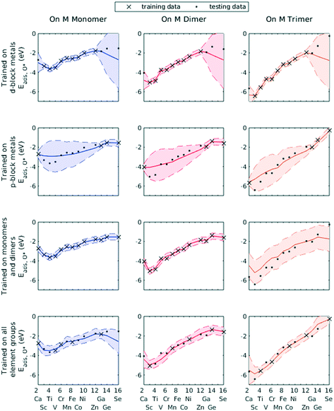
We demonstrated this by selecting all d-block metals to be in the training set and leaving all p-block metals for the testing set. The GPR model, using identical hyperparameters to previous trials, failed to accurately predict the O* adsorption energy for most p-block metals (Fig. 7, row 1). Similarly, using only p-block metals as training data, the GPR model could not estimate for d-block metals (Fig. 7, row 2). However, wherever the GPR model failed to make accurate predictions, the corresponding variance in the conditional probability distribution enlarged, indicating less confidence in the estimated values. Similarly, when only including data on Cu–Cu–M sites and Cu–M–M sites in the training set, GPR prediction on M–M–M gave a large confidence interval (Fig. 7, row 3). A lack of knowledge of any feature can be effectively taken into account by the GPR algorithm. Finally, when including all element groups into the training set, a reasonable confidence interval was achieved throughout the testing set (Fig. 7, row 4).
3.5 Selecting training data intelligently with active learning
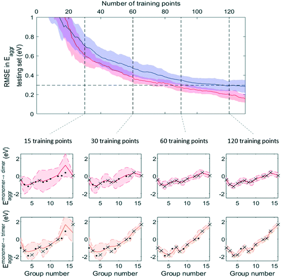
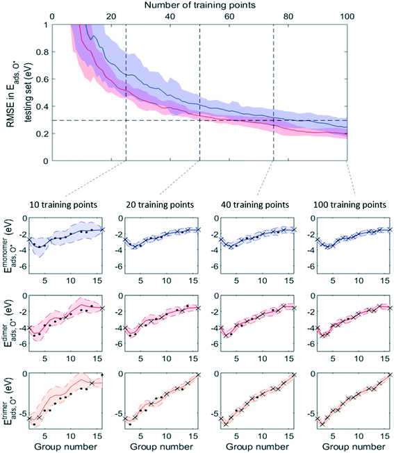
The large impact of training set selection on ML model performance (sec. 3.3.2) necessitates effective selection of its data in order to reduce training time and improve ML accuracy. One approach is to use human intuition to guide the selection and maximize the model's exposure to diverse data. While certainly feasible, this would imply more human efforts and inevitable human bias. Alternatively, recent ML works have focused on use of active learning in automated ML training, such as in electronic structure calculations.49,50Active learning algorithms refer to ML schemes where the machine automatically queries the user (DFT program, in our case) in order to achieve good model training using a minimal amount of training data. The convenient feature of uncertainty estimation of GPR enables straight-forward implementation of active learning, whereby data points with the highest predictive variances are selected as the next training data. This is because data with the highest variance represents the most uncertainty, and learning from this data maximizes the ML model's information gain. We subsequently sampled our chemical space with active learning.
Fig. 7 and 8 show that, while RMSE on testing sets decreased as more data was added to the training set for both active learning-enabled ML model and random-selecting ML model, active learning helped RMSE decrease much more rapidly. In the case of Eaggr prediction, in order to achieve an RMSE of 0.3 eV (average RMSE with random shuffling), an active learning agent could reach this using around 85 training points, whereas the randomly selecting agent needed 120 (about 3/4 of total data points) to reach it. The active learning agent hence resulted in a one third time saving. Similarly, for Eads,O* prediction, active learning required only 60 training points whereas random selection required 90; also a one third time saving.
Note that to eliminate possible bias from the random staring point, we averaged 50 trials, using different starting points, and show the average curve in Fig. 8 and 9 together with the standard deviation shown as the shaded areas. By examining one of these 50 trials, we plotted the ML prediction on period 4 elements and observed that at lower number of training points, the ML prediction generally yielded large uncertainty. This uncertainty decreased as more training data was added. During this process, active learning tended to select training points that were most dissimilar to existing training data, in line with the objective of maximizing the ML model's information gain. Throughout the training process, almost all predictions were within the ±2σ confidence interval (shaded areas), affirming the GPR model's ability to quantify uncertainty accurately.
3.6 Transferability of ML model and active learning process
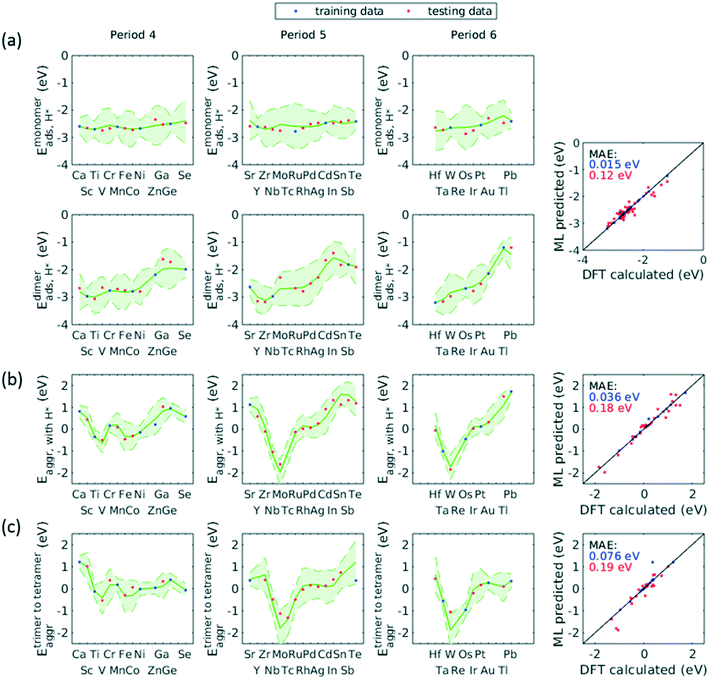
The applicability of the ML model to a broad range of applications required assessment of the ML model's transferability beyond the Cu substrate, O* adsorbate, and trimer cluster size. We accordingly used the trained GPR model to predict for additional substrates, adsorbate, and cluster size. As discussed in sec. 3.4, for data with some specific characteristics (e.g. d-block metals, monomers), the GPR model would yield large prediction uncertainty if not trained on any of these data. This holds true for the extra dimensionalities to be studied in this transferability assessment. We therefore extended our original dataset to include these new dimensions. In order to minimize the number of new DFT calculations, we employed the same active learning algorithm to select the training data on the aforementioned dimensionalities.To describe the additional features, we concatenated the original features and the new features. For additional substrates, we included nine precious metals into our dataset (Ru, Rh, Pd, Ag, Re, Os, Ir, Pt, Au) while fixing the dilute metal as Ni, and the same method describing the dilute metal were used to describe the substrate (i.e. atomic number, group number, period number, electronegativity, and atomic radius). For additional adsorbate, we included H* and used one hot encoding to represent this new adsorbate. For additional cluster size, we included tetramers of the same 38 elements and simply incremented the original cluster size feature to describe the tetramer. Adsorbate-induced effects in tetramers and larger clusters would complicate the model as the location of adsorbate becomes important, and would require significantly more feature engineering. Therefore, we only evaluated clean tetramers of 38 elements in current study.
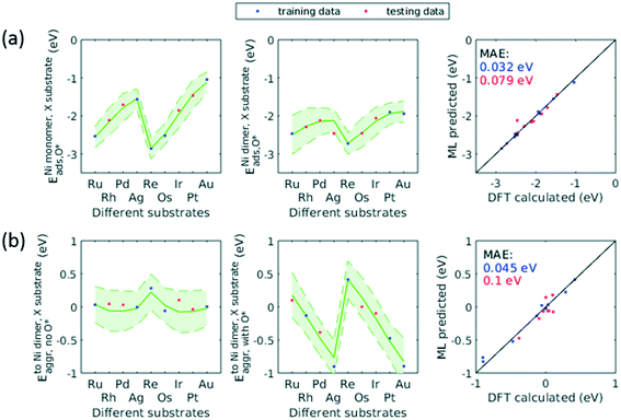
When trained on only a third of the data for H* adsorbate (Fig. 10a) and tetramers (Fig. 10b), the updated GPR model gave a testing MAE of no more than 0.2 eV. When half of the data were included in the training set, the performance approached that of original GPR model (0.1 eV). The smaller required training data size indicated that patterns in the original data learned by the GPR model were transferred to predicting the new dimensionalities, thereby reducing number of training data needed and significantly accelerating the screening process. On the other hand, when predicting for other substrates (Fig. 11), the testing MAE did not become reasonably small until trained on 1/2 of the data. This is probably due to the small total number of data available. After trained on 1/2 data, the MAE became as small as 0.1 eV. We note that throughout the active learning process, both training and testing data set always lied within the 95% confidence interval. Accordingly, when extending this model to unknown chemical space, the prediction uncertainty can be utilized to reliably assess if sufficient training data are fed to the model.
4. Conclusion and future work
Despite significant progress in ML-assisted catalyst design, the majority of ML models predict only for adsorption energy, but not for the stability of the assumed active sites, particularly those that could change due to adsorbate effects. To bridge this gap, we built a GPR-based ML model to predict aggregation energies of single-atom alloy sites (both clean and O* adsorbed surfaces) and the O* adsorption energies on these sites. We calculated initial and final energy values using DFT. The complexity in the periodic trends in our DFT results led us to utilize and compare three different non-parametric ML models: Gaussian kernel regression (GKR), Gaussian kernel-based support vector machine (SVM) and Gaussian process regression (GPR). Among these, GPR exhibited the best performance and was most suitable for our data, yielding an RMSE of 0.30 eV, a MAE of 0.09 eV and an R2 greater than 0.9 for both aggregation and adsorption energy testing sets.The additional advantage of GPR's uncertainty quantification ability enabled us to understand the effect of selecting training datasets, based on which we further optimized our GPR model and reduce the error below the average error achieved through random selection of training datasets. We found that selecting training datasets such that predicted elements (in testing sets) are of similar nature to those in training sets significant boosts model performance. Based on this principle, we utilized an active learning algorithm to automatically select training data, which saved approximately a third of training time compared to random selection of training data.
Promisingly, the GPR model possesses significant transferability and can extend to additional degrees of freedom (substrates, adsorbates, and larger cluster sizes) using a small training set. This provides an important advantage as the immense chemical space cannot be practically calculated using DFT. By employing the GPR model, there is potentially an orders of magnitude of reduction in computational time as GPR models are evaluated quickly. For future work, we aim to incorporate detailed descriptors for different adsorbates21 (such as CO*, OH* or CHOH*) and arbitrary surface structures and subsurface alloys.
Conflicts of interest
There are no conflicts to declare.Acknowledgements
We sincerely thank Erwin Edward Hart Professorship, Natural Sciences and Engineering Research Council of Canada (NSERC, RGPIN-2018-04642), and University of Toronto for financial supports. We additionally thank Compute Canada for the computational infrastructure.References
- E. Roduner, Chem. Soc. Rev., 2014, 43, 8226–8239 RSC.
- International Energy Agency, Tracking Progress: Industry, 2017 Search PubMed.
- Y. J. Pagán-Torres, J. Lu, E. Nikolla and A. C. Alba-Rubio, in Studies in Surface Science and Catalysis, Elsevier Inc., 2017, vol. 177, pp. 643–676 Search PubMed.
- U. Bardi, Rep. Prog. Phys., 1994, 57, 939–987 CrossRef CAS.
- J. Greeley and M. Mavrikakis, Catal. Today, 2006, 111, 52–58 CrossRef CAS.
- R. Ghosh Chaudhuri and S. Paria, Chem. Rev., 2012, 112, 2373–2433 CrossRef CAS.
- A. Wang, J. Li and T. Zhang, Nat. Rev. Chem., 2018, 2, 65–81 CrossRef CAS.
- J. Greeley, I. E. L. Stephens, A. S. Bondarenko, T. P. Johansson, H. A. Hansen, T. F. Jaramillo, J. Rossmeisl, I. Chorkendorff and J. K. Nørskov, Nat. Chem., 2009, 1, 552–556 CrossRef CAS.
- J. Greeley and J. K. Nørskov, Surf. Sci., 2007, 601, 1590–1598 CrossRef CAS.
- J. K. Nørskov, F. Abild-Pedersen, F. Studt and T. Bligaard, Proc. Natl. Acad. Sci. U. S. A., 2011, 108, 937–943 CrossRef.
- B. R. Goldsmith, J. Esterhuizen, J.-X. Liu, C. J. Bartel and C. Sutton, AIChE J., 2018, 64, 2311–2323 CrossRef CAS.
- T. Toyao, K. Suzuki, S. Kikuchi, S. Takakusagi, K. I. Shimizu and I. Takigawa, J. Phys. Chem. C, 2018, 122, 8315–8326 CrossRef CAS.
- I. Takigawa, K. I. Shimizu, K. Tsuda and S. Takakusagi, RSC Adv., 2016, 6, 52587–52595 RSC.
- Z. Li, S. Wang, W. S. Chin, L. E. Achenie and H. Xin, J. Mater. Chem. A, 2017, 5, 24131–24138 RSC.
- C. J. Baddeley, L. H. Bloxham, S. C. Laroze, R. Raval, T. C. Q. Noakes and P. Bailey, J. Phys. Chem. B, 2002, 105, 2766–2772 CrossRef.
- I.-H. Svenum, J. A. Herron, M. Mavrikakis and H. J. Venvik, Catal. Today, 2012, 193, 111–119 CrossRef CAS.
- K. J. J. Mayrhofer, V. Juhart, K. Hartl, M. Hanzlik and M. Arenz, Angew. Chem., Int. Ed., 2009, 48, 3529–3531 CrossRef CAS.
- M. Moskovits and B. Vlčková, J. Phys. Chem. B, 2005, 109, 14755–14758 CrossRef CAS.
- T. Kim, C. H. Lee, S. W. Joo and K. Lee, J. Colloid Interface Sci., 2008, 318, 238–243 CrossRef CAS PubMed.
- A. V. Ruban, H. L. Skriver and J. K. Nørskov, Phys. Rev. B: Condens. Matter Mater. Phys., 1999, 59, 15990–16000 CrossRef.
- C. A. Menning and J. G. Chen, J. Chem. Phys., 2009, 130, 174709 CrossRef.
- A. Christensen, A. Ruban, P. Stoltze, K. Jacobsen, H. Skriver, J. Nørskov and F. Besenbacher, Phys. Rev. B: Condens. Matter Mater. Phys., 1997, 56, 5822–5834 CrossRef CAS.
- P. E. Blöchl, Phys. Rev. B: Condens. Matter Mater. Phys., 1994, 50, 17953–17979 CrossRef PubMed.
- J. P. Perdew, K. Burke and M. Ernzerhof, Phys. Rev. Lett., 1996, 77, 3865–3868 CrossRef CAS.
- R. Ouyang, J. X. Liu and W. X. Li, J. Am. Chem. Soc., 2013, 135, 1760–1771 CrossRef CAS.
- Y. Q. Su, Y. Wang, J. X. Liu, I. A. W. Filot, K. Alexopoulos, L. Zhang, V. Muravev, B. Zijlstra, D. G. Vlachos and E. J. M. Hensen, ACS Catal., 2019, 9, 3289–3297 CrossRef CAS.
- K. G. Papanikolaou, M. T. Darby and M. Stamatakis, J. Phys. Chem. C, 2019, 123, 9128–9138 CrossRef CAS.
- M. T. Darby, E. C. H. Sykes, A. Michaelides and M. Stamatakis, Top. Catal., 2018, 61, 428–438 CrossRef CAS.
- K. Yang and B. Yang, Phys. Chem. Chem. Phys., 2017, 19, 18010–18017 RSC.
- J. C. Slater, J. Chem. Phys., 1964, 41, 3199–3204 CrossRef CAS.
- L. Pauling, J. Am. Chem. Soc., 1932, 54, 3570–3582 CrossRef CAS.
- Z. Li, X. Ma and H. Xin, Catal. Today, 2017, 280, 232–238 CrossRef CAS.
- F. R. Lucci, T. J. Lawton, A. Pronschinske and E. C. H. Sykes, J. Phys. Chem. C, 2014, 118, 3015–3022 CrossRef CAS.
- M. B. Boucher, B. Zugic, G. Cladaras, J. Kammert, M. D. Marcinkowski, T. J. Lawton, E. C. H. Sykes and M. Flytzani-Stephanopoulos, Phys. Chem. Chem. Phys., 2013, 15, 12187–12196 RSC.
- M. T. Kief and W. F. Egelhoff, Phys. Rev. B: Condens. Matter Mater. Phys., 1993, 47, 10785–10814 CrossRef CAS.
- W.-D. Kang, Y.-C. Wei, C.-W. Liu and K.-W. Wang, Electrochem. Commun., 2011, 13, 162–165 CrossRef CAS.
- N. Inoǧlu and J. R. Kitchin, Phys. Rev. B: Condens. Matter Mater. Phys., 2010, 82, 045414 CrossRef.
- S. Bhattacharjee, U. V. Waghmare and S. C. Lee, Sci. Rep., 2016, 6, 35916 CrossRef CAS.
- S. Schnur and A. Groß, Phys. Rev. B: Condens. Matter Mater. Phys., 2010, 81, 033402 CrossRef.
- H. Xin, A. Vojvodic, J. Voss, J. K. Nørskov and F. Abild-Pedersen, Phys. Rev. B: Condens. Matter Mater. Phys., 2014, 89, 115114 CrossRef.
- Z. W. Ulissi, A. J. Medford, T. Bligaard and J. K. Nørskov, Nat. Commun., 2017, 8, 14621 CrossRef.
- R. Jinnouchi and R. Asahi, J. Phys. Chem. Lett., 2017, 8, 4279–4283 CrossRef CAS.
- X. Ma, Z. Li, L. E. K. Achenie and H. Xin, J. Phys. Chem. Lett., 2015, 6, 3528–3533 CrossRef CAS.
- Z. Li, N. Omidvar, W. S. Chin, E. Robb, A. Morris, L. Achenie and H. Xin, J. Phys. Chem. A, 2018, 122, 4571–4578 CrossRef CAS PubMed.
- I. M. Sobol, Math. Comput. Simul., 2001, 55, 271–280 CrossRef.
- J. Cui and R. V. Krems, J. Phys. B: At., Mol. Opt. Phys., 2016, 49, 224001 CrossRef.
- K. Lejaeghere, V. Van Speybroeck, G. Van Oost and S. Cottenier, Crit. Rev. Solid State Mater. Sci., 2014, 39, 1–24 CrossRef CAS.
- S. H. Lee and W. Chen, Struct. Multidiscipl. Optim., 2009, 37, 239–253 CrossRef.
- E. Uteva, R. S. Graham, R. D. Wilkinson and R. J. Wheatley, J. Chem. Phys., 2018, 149, 174114 CrossRef PubMed.
- J. Noh, S. Back, J. Kim and Y. Jung, Chem. Sci., 2018, 9, 5152–5159 RSC.
Footnote |
| † Electronic supplementary information (ESI) available. See DOI: 10.1039/c9cy02070e |
| This journal is © The Royal Society of Chemistry 2020 |


