 Open Access Article
Molecular free energy optimization on a computational graph†
Xiaoyong Caoa and
Pu Tian *ab
*ab
aSchool of Life Sciences, Jilin University, Changchun, 130012, China. E-mail: tianpu@jlu.edu.cn; Tel: +86 431 85155287
bSchool of Artificial Intelligence, Jilin University, Changchun, 130012, China
First published on 6th April 2021
Abstract
Free energy is arguably the most important property of molecular systems. Despite great progress in both its efficient estimation by scoring functions/potentials and more rigorous computation based on extensive sampling, we remain far from accurately predicting and manipulating biomolecular structures and their interactions. There are fundamental limitations, including accuracy of interaction description and difficulty of sampling in high dimensional space, to be tackled. Computational graph underlies major artificial intelligence platforms and is proven to facilitate training, optimization and learning. Combining autodifferentiation, coordinates transformation and generalized solvation free energy theory, we construct a computational graph infrastructure to realize seamless integration of fully trainable local free energy landscape with end to end differentiable iterative free energy optimization. This new framework drastically improves efficiency by replacing local sampling with differentiation. Its specific implementation in protein structure refinement achieves superb efficiency and competitive accuracy when compared with state of the art all-atom mainstream methods.
Introduction
Full understanding of free energy landscape (FEL) for a given molecular system implicates the ability to accurately predict its behavior, and provides a rational basis for further manipulation and design. Scientists have made tremendous effort in calculating FEL with great achievements in advancement of both theory and computational algorithms.1 Rigorous computation of FEL usually involves sampling of configurational space by molecular simulations and post-processing of generated trajectories/statistics. More efficient estimation as utilized in design/prediction/refinement of protein structures2–4 involves repetitive proposal/sampling and/or energy minimization of candidate structures/sequences (e.g. FastRelax5) followed by evaluating/scoring with various forms of potentials.6–8 All these schemes have fundamental limitations as briefed below:(1) Pairwise approximation of non-bonded molecular interactions is utilized in essentially all molecular modeling with either physics or knowledge based force fields (FF) (e.g. CHARMM,9 Rosetta10). Two non-bonded basic units (atoms or coarse grained particles) are assumed to have interactions determined only by the distance (and orientation in case of anisotropic units) between them, regardless of identity and spatial distribution of other neighboring units.
(2) Fixed simple functional form (e.g. Lennard-Jones, quadratic form) are utilized in traditional FF for convenience of fitting. While having well grounded physical underpinning when relevant basic units are near equilibrium positions (local minima), these functions create a ceiling of accuracy for description of frustrated molecular systems11 with a significant fraction of comprising units off energy minima position and/or orientation.
(3) Repetitive local sampling is universal. The number of energetically favorable local configurations of a given composition for typical molecular systems (e.g. water, protein) at specific conditions (e.g. temperature, pressure) is a tractable number and form a local FEL (LFEL). The reason is that local correlations are strong in soft condensed matter, thus effective local dimensionality is much smaller than that corresponds to the number of degrees of freedom (DOFs). Different local compositions, which is also a tractable number for similar reason, form different LFEL. Competition and superposition of these overlapping LFEL constitutes global FEL of a given molecular system. However, sampling of these local arrangements are repeatedly carried out with tremendous wasting of computational resources.
(4) No direct manipulation of molecular coordinates based on free energy is available for sampling based methods.
(5) Maintenance of rigid constraints (e.g. bond lengths) is frequently utilized to improve efficiency of molecular simulations with either shake,12 rattle13 or settle14 algorithm. These iterative procedures maintain bond lengths (and angles) within a preset tolerance off target value, engender computational cost, and may diverge when large forces are experienced by relevant units. Specialized methods, such as concerted rotation15 and backrub,16 are helpful in maintaining constraints for stochastic configurational space sampling of (bio)polymers. However, these procedures may not be directly driven by differentiation w.r.t. (with respect to) a given potential.
Among these limitations, the first two have fundamental impact on accurate interaction description, the third and the fourth severely decrease computational efficiency, and the fifth is a nuisance. Neural network based many body potentials17 may help with the first two limitations. The remaining three are yet to be overcome. We previously developed generalized solvation free energy (GSFE) theory.8 The local maximum likelihood approximation (LMLA) of GSFE theory was implemented with a simple neural network to assess protein structural models, and demonstrated strong competitiveness when compared with state-of-the-art knowledge based potentials. The physical essence of GSFE is caching of LFEL by training with data sets derived from high resolution experimental structures. The connection of LFEL to mainstream enhanced sampling and coarse-graining algorithms are described in detail elsewhere.18
A graph is a set of vertices and edges connecting them. In a computational graph, vertices are functions that processing data transmitted through edges. Autodifferentiation (AD) is a powerful way of solving exact derivatives first developed in 1974,19 its special form of backpropagation (BP) in neural network was reinvented by Hinton20 in 1986. Derivatives, as long as they exists, in all programmable computational process may be calculated with autodifferentiation without explicit functional forms. The gorgeous capability of computational graph empowered by autodifferentiation has been proven by widespread application of major artificial intelligence platforms (e.g. TensorFlow and PyTorch). Integrating the GSFE theory, coordinates transformation and autodifferentiation, we map molecular free energy optimization onto a computational graph to address the last three of above mentioned challenges. Implementation of this algorithm in protein structure refinement (PSR) is demonstrated to be competitive in accuracy and orders of magnitude more efficient when compared with present mainstream methodologies.
Methods
Introduction to local maximum likelihood approximation of GSFE
In GSFE, each comprising unit is both solute and solvent of its neighbors. For a n-residue protein with sequence X = {x1, x2, …, xn}, the free energy of a given structure is:
F = −ln![[thin space (1/6-em)]](https://www.rsc.org/images/entities/char_2009.gif) P(Structure|X) P(Structure|X)
| (1) |
With Bayes formula:
−ln![[thin space (1/6-em)]](https://www.rsc.org/images/entities/char_2009.gif) P(Structure|X) = −ln P(Structure|X) = −ln![[thin space (1/6-em)]](https://www.rsc.org/images/entities/char_2009.gif) P(X|Structure)P(Structure)/P(X) P(X|Structure)P(Structure)/P(X)
| (2) |
For a given sequence X, P(X) is a constant and is dropped. For maximum likelihood approximation, the prior term P(Structure) is ignored. Define Ri(Xi, Yi) as local structural regions within selected cutoff distance of Xi (Yi being specific solvent of Xi). With further local approximation we have:
 | (3) |
Eqn (3) assumes all influence to each unit is included in its solvent Yi, this product of n local likelihood terms is the LMLA (local maximum likelihood approximation) of GSFE, which is the basis for our NN training in this work. Incorporation of local priors and direct long range interactions will be tackled in future.
Training of local free energy landscape neural network
The same training/validation/test dataset as ref. 8 is used for training LFEL. For each target residue, 22 neighboring residues are selected as its neighbors (6 upstream, 6 downstream sequentially adjacent residues in primary sequence and 10 non-adjacent ones). Features for each target residue include one-hot vectors representing identities of neighboring residues, residue pair distances (Cα–Cα) between the target and its neighbor residues, and dihedral angles (Cα, C, N, Cβ) indicating side chain orientations. Input for each comprising solvent unit of a LFEL includes a 22-dimensional one-hot vector, 6 sets of bond angle parameters (each angle θ is converted into sin![[thin space (1/6-em)]](https://www.rsc.org/images/entities/char_2009.gif) θ and cos
θ and cos![[thin space (1/6-em)]](https://www.rsc.org/images/entities/char_2009.gif) θ), and the Cα–Cα distance resulting in an input of (22 + 6 × 2 + 1) × 22 = 770 dimensions, the resulting LFEL is denoted as 770-LFEL. A four-layer feed-forward (770-512-512-512-21) network architecture is used (Fig. 2A) and trained for 30 epochs with a learning rate of 0.1.
θ), and the Cα–Cα distance resulting in an input of (22 + 6 × 2 + 1) × 22 = 770 dimensions, the resulting LFEL is denoted as 770-LFEL. A four-layer feed-forward (770-512-512-512-21) network architecture is used (Fig. 2A) and trained for 30 epochs with a learning rate of 0.1.
Refinement datasets
Four data sets are prepared to evaluate GSFE-refinement. The first is 3DRobot data set. After removing structures having sequences of higher than 25% identity with training set, 36 of original 200 native structures21 remain, and 322 decoys for these 36 native structures are selected by random sampling according to refineD.22 The second is the 150-target refineD test set.22 The third dataset includes 34 decoys available from CASP11 and 31 available from CASP12 respectively. The last data set is the 31 decoys out of 44 from CASP14 (we missed the earliest 13 targets due to late registration). CASP decoys are downloaded from CASP website (https://predictioncenter.org/download_area/).The refinement pipeline
As shown in Fig. 2B, a given starting structure is first striped of all side chain atoms other than Cβ. Cartesian coordinates of the remaining backbone (Cα, CO, N) and Cβ atoms are converted into internal coordinates, which is further converted back into Cartesian coordinates for feature extraction. The NeRF (Natural Extension Reference Frame) algorithm (see ESI for details†) is used for coordinates transformation in both ways (see ESI for details†). The approximate free energy calculated by the forward pass through the neural network (which caches LFELs), plus some additional restraints (see below), constitute the total loss function. Derivatives of the total loss w.r.t. the input coordinates is calculated with back propagation of AD, and optimization is subsequently performed with simple gradient descent using the given learning rate and calculated derivatives. To maintain constraints of bond lengths and angles, only gradients of the loss function w.r.t. backbone dihedrals ϕ and ψ are saved, and derivatives w.r.t. other inputs are set to zero.| LOSS = loss + λlosssmoothL1 | (4) |
 | (5) |
 | (6) |
 | (7) |
Results
Mapping of free energy optimization onto a computational graph
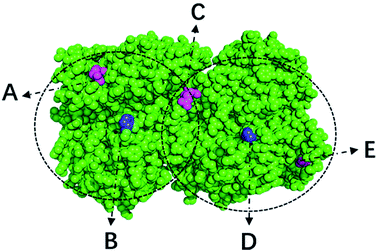
With a simple probabilistic description of molecular systems, GSFE formulates a directed link from molecular coordinates to LFEL, superposition of which under strict implicit global correlation restraints (see eqn (3) and Fig. 1) is utilized to approximate total free energy of interested molecular system. Caching of LFEL through training of the neural network is described perviously8 (and briefed in Methods section as well). However, GSFE does not provide measures to efficiently update structures. In principle, with establishment of a computational graph, BP operation of AD from calculated approximate free energy (AFE) to coordinates may provide gradients (and higher ordered derivatives when needed) of AFE w.r.t. coordinates, which may subsequently be updated by a simple gradient descent (or higher ordered) optimization. AD is implemented by major AI platforms and may be turned on by a simple statement. One concern is that in such direct update of coordinates, bond lengths/angles would be changed and one has to utilize iterative algorithms such as shake12 or rattle13 to maintain constraints if desire. To overcome this issue, we design a coordinate transformation procedure that updates internal coordinates where only derivatives w.r.t. interested quantity (dihedrals) are utilized and derivatives w.r.t. constraint quantity (bond lengths and angles) are set to zero. This way, constraints are realized exactly with no concern of divergence. As shown in Fig. 2, to facilitate feature extraction, a transformation from internal to Cartesian coordinates is necessary.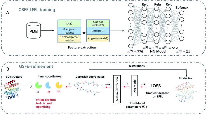 | ||
| Fig. 2 Schematic representation of GSFE-refinement training and optimization. (A) Illustration of LFEL training based on LMLA-GSFE (see ref. 8 for details). (B) Illustration of the fully end-to-end differentiable optimization pipeline. Small solid black arrows represent forward pass computation of approximate free energy, small solid red arrows represent BP operation for taking derivatives. The empty arrow represents input of decoys. Final result is delivered as output after a preset iteration number N. | ||
GSFE-refinement performance on 3DRobot data set
| LR/λ/Wa | Avg-ΔGDT-HAb | GDT-HA-numc | Avg-ΔRMSDd | RMSD-nume |
|---|---|---|---|---|
| a LR is the learning rate, λ is the coefficient of smooth_l1 loss for conformation restraints, W is the AA weight (see eqn (5) and (6), with 1 represents on and 0 represents off).b The average value of ΔGDT-HA for all decoys.c The average number of decoys with ΔGDT-HA > 0 for all 36 decoy sets.d The average value of ΔRMSD for all decoys.e The average number of decoys with ΔRMSD < 0 for all 36 decoy sets. | ||||
| 0.001/0/0 | −1.38 | 95/322 | 0.0022 | 130/322 |
| 0.0005/0/0 | −0.18 | 134/322 | −0.0175 | 158/322 |
| 0.0001/0/0 | 0.2 | 182/322 | −0.0099 | 201/322 |
| 0.0005/0.1/0 | −0.19 | 137/322 | −0.0168 | 166/322 |
| 0.0005/1.2/0 | −0.02 | 162/322 | −0.0147 | 188/322 |
| 0.0005/10.0/0 | 0.24 | 211/322 | −0.0167 | 257/322 |
| 0.0005/0.1/1 | 0.02 | 163/322 | −0.0136 | 191/322 |
| 0.0005/1.2/1 | 0.26 | 214/322 | −0.0178 | 275/322 |
| 0.0005/10.0/1 | 0.27 | 210/322 | −0.019 | 291/322 |
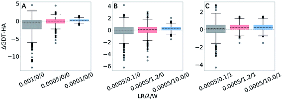 | ||
| Fig. 3 Box plots for ΔGDT-HA with different LR/λ/W combinations for 3DRobot dataset. Effects of variation are exhibited for (A) learning rates, (B) structural restraints and (C) weights for approximating local priors. More box plots of ΔRMSD and ΔGDT-HA are available in ESI (Fig. S1–S3).† | ||
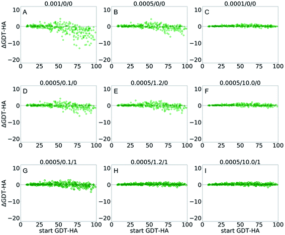 | ||
| Fig. 4 Scatter plots of AΔGDT-HA as a function of start GDT-HA score for best of top 5 models from GSFE-refinement for 3DRobot dataset. Corresponding LR/λ/W combination is noted on top of each plot. Effects of variation are exhibited for (A–C) learning rates; (D–F) structural restraints and (G–I) weights for approximating local priors. More scattered plots of ΔRMSD and ΔGDT-HA are available in ESI (Fig. S4–S6).† | ||
GSFE-refinement performance on refineD data set
In order to further investigate the robustness of GSFE-refinement, we test its performance on the refineD dataset at LR/λ/W = 0.0005/1.2/1 with 770-LFEL. As shown in Table 2 (see detailed results in Tables S1 and S2 in ESI†), in top 1 models, the GDT-HA score of GSFE-refinement is 0.08 and ranks the fourth. In best of top 5 models, GSFE-refinement ranks the sixth, its result (0.4400) is better than FastRelax-0.5 Å (0.0548), FastRelax-4.0 Å (0.0751), FastRelax (−0.1999), ModRefiner-0 (−0.8400), and ModRefiner-100 (0.1491). These results are generated by 5 iterations within a few seconds on a single CPU core, in strong contrast to conventional sampling and minimization (e.g. FastRelax5) where thousands or even hundreds of thousands of iterations and hours of CPU time are usually necessary. It is also important to note that despite all heavy atom in side chains other than Cβ are missing in our model, competitive accuracy is achieved when compared with state-of-the-art full heavy atom methods. However, the superior efficiency is mainly due to substitution of local sampling by differentiation. The number of atoms in GSFE-refinement is more than half of all heavy atoms.| Method | Avg. top 1 | Avg. best of 5 | GDT-HA-num |
|---|---|---|---|
| a More details for top 1 and the best of top 5 models for refineD data set are available in ESI (Tables S1 and S2). | |||
| refineD-C | 0.6365 | 1.3109 | 121/150 |
| refineD-NC | −1.2403 | 1.5343 | 104/150 |
| FG-MD | 0.5597 | 0.5597 | — |
| FastRelax | −3.4317 | −0.1999 | — |
| FastRelax-0.5 Å | −0.3411 | 0.8811 | 90/150 |
| FastRelax-2.0 Å | −1.2120 | 0.8223 | 77/150 |
| FastRelax-4.0 Å | −2.5471 | 0.0751 | 67/150 |
| ModRefiner-0 | −0.8400 | −0.8400 | — |
| ModRefiner-100 | 0.1491 | 0.1491 | — |
| GSFE-refinement | 0.0800 | 0.4400 | 112/150 |
GSFE-refinement performance on CASP11 and CASP12 data set
GSFE-refinement is further evaluated on the CASP11 and CASP12 dataset (see Methods). Based on above mentioned results, we utilize a parameter combination LR/λ/W = 0.0005/1.2/1. In Fig. 5, we present structural change of the CAPS11 and CASP12 decoys after GSFE-refinement as measured by ΔGDT-HA and ΔRMSD, and improvement is observed for most of the cases. Specifically, there are 50% (17/34) and 88.2% (30/34) successful refinement when evaluated by GDT-HA and RMSD scores in CASP11 (as shown in Fig. 5A and B), and 64.5% (20/31) and 100% (31/31) when evaluated by GDT-HA and RMSD scores in CASP12 (as shown in Fig. 5C and D) (see detailed results in Tables S3–S6 and Fig. S7 in ESI†).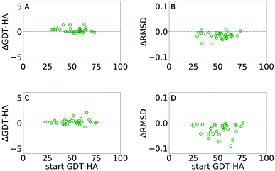 | ||
| Fig. 5 ΔGDT-HA and ΔRMSD of best of top 5 models as a function of start GDT-HA score obtained from GSFE-refinement of CASP11 (A and B) and CASP12 (C and D) datasets. Corresponding plots for top 1 models are presented in ESI (Fig. S7).† | ||
GSFE-refinement assessment in CASP14
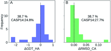
We participated in CASP14 competition and submitted 180 models for 36 targets (we registered late and missed the first 13 targets), among which 31 are effective targets in CASP14 final statistics. As shown in Fig. 6, we improved 38.7% targets compared with the 24.8% of CASP14 average as measured by ΔGDT-HA, and improved 38.7% targets compared with the 27.7% average as measured by ΔRMSD_CA. In top 1 model, GSFE-refinement (with GR code 294) ranks 12 according to SUM Z score (>0.0) based on GDT-TS score. And AVG Z score (>0.0) based on GDT-TS score ranks 6 (https://predictioncenter.org/casp14/zscores_final_refine.cgi). Specific Z scores of GSFE-refinement is provided in ESI Fig. S9.† In particular, for 13 targets with start GDT-TS score better than 60, GSFE-refinement ranks the first. Again, we performed 5 iterations for each target, with computing cost ranging from 0.7 to 2.7 seconds on a single CPU core (R1028 has 75 amino acids and costs 0.7 s. R1042v1 contains 276 amino acids, which takes 2.7 s).Discussions
Optimization of molecular free energy on a computational graph proposed and demonstrated in this work makes two distinct contributions,(1) Replacement of expensive local sampling by differentiation w.r.t. cached LFEL realizes superb efficiency.
(2) Combination of AD and coordinate transformation realizes exact hard constraints with minimal computational cost.
GSFE-refinement takes a few seconds on a single CPU core for refinement of typical decoys, in strong contrast to hours for typical sampling and energy minimization with knowledge based potential (e.g. FastRelax5) without explicit water representation, and thousands or even tens of thousands hours for refinement based on MD simulations with explicit water representation. As backbone and Cβ atoms are more than half of all heavy atoms, speed-up due to smaller number of atoms is relatively insignificant, and replacement of local sampling by differentiation is the key underlying its efficiency. GSFE-refinement is, to the best of our knowledge, the first end-to-end differentiable algorithm that takes fully trainable parameters and can generate a continuous dynamic trajectory similar to MD simulation. This unique property make it possible to realize physics based ab initio folding when properly trained for both unfolded and folded states, while likely to be significantly more efficient than MD simulation based folding.33,34 The competitive accuracy of our backbone and Cβ representation on a par with mainstream all atom methods suggest that many body correlation captured by GSFE-refinement are important. Simple backbone and Cβ representation provides additional benefit of smoother FEL than all atom counterpart, its value in this regard is irreplaceable despite higher expected accuracy of all atom LFEL that is under development in our group. It is important to note that GSFE theory is one way of implementing LFEL for global free energy estimation and there might well be more elegant ways. While only gradient descent optimization is demonstrated in this work, AD is capable of calculating exact higher ordered derivatives and therefore exploration of higher ordered optimization algorithms in this scheme is certainly feasible and will be carried out in the future.
To cache or to compute intermediate results on the fly is a ubiquitous tradeoff in computation. As far as molecular free energy is concerned, we rely far more than necessary on computing by sampling, and much less on the inexpensive memory. “Local” in this work is conveniently defined as specific solvent units of each solute unit and its spatial coverage (i.e. cutoff) need to be determined to implement GSFE for construction of LFEL. The larger the “local” is, the more data and the larger neural networks are needed to cache corresponding LFEL, and the faster and more accurate computation will be achieved in subsequent free energy optimization. However, as strength of correlation decreases rapidly with distance, when “local” extends beyond certain level of correlation, the increase of data and training cost is likely to be unworthy and negative impact of noises may rise. Input for training LFEL may be of either computational or experimental origin. Apart from hardware consideration for the optimization, data availability and network architecture are of critical importance for training. In the case of PSR presented here, the size of the “local” is likely restricted either by the number of available high resolution experimental structures or by efficiency of network in extracting correlations. If significantly more surrounding residues were taken as the solvent of a target residue, reliable description of their spatial distributions would require more data and/or more efficient network. More investigations are necessary to understand relative importance of these two factors. When high quality experimental data is not available or not sufficient, a potentially feasible two-step strategy is to first utilize neural network FF to generate sufficiently large number of configurations for interested compositions at desired thermodynamic conditions (e.g. temperature and pressure). This step, if done properly, may realize sampling of reliable quantum mechanical accuracy. Secondly, these configurations may be subsequently utilized to construct LFEL for efficiently and reliably carrying out many free energy optimization tasks with near quantum accuracy and efficiency of traditional coarse grained methods. For proteins in particular, complete computation driven ab initio folding of proteins without learning from experimental structural information is potentially possible in this framework.
In eqn (3), all local distributions seem be treated as independent. However, this is not the case in our implementation. Apart from direct long-range interactions, all mediated global correlations among overlapping local regions are embodied by the fact that they share the same coordinates. This constraint is exactly satisfied during all iterations as only one set of coordinates are utilized. At each cycle, each residue participating in LFEL of all its solvent units and its coordinates are updated as a result of compromise among their LFEL, result in a larger effective cutoff than defined by “local” in training of LFEL (see Fig. 1).
One great feature of our scheme is that coordinate update and transformation module is separated from LFEL. Therefore, future modification of neural network architecture for caching LFEL is flexible. For the specific task of PSR and its potential extension to ab initio protein folding, we indeed need such flexibility to advance from present backbone and Cβ level LMLA treatment (eqn (3)) to incorporate all side chain heavy atoms, local priors and direct long range interactions. Another advantage of GSFE is that direct control of each comprising unit is straight forward with well-defined physical interpretation as demonstrated by addition of local restraints (eqn (5) and (6)). The scheme (Fig. 2) for optimizing molecular free energy on a computational graph is of general utility in soft matter modeling. It is also important that while brute force caching of LFEL is apparently specific for given constraint environmental conditions (e.g. temperature, pressure, composition), inclusion of these conditions within LFEL is possible and will be one interesting future research direction.
In light of the amazing success by AlphaFold2 for protein structure prediction, it is important to note that our algorithm is targeted to physical simulation and understanding of both static distributions (i.e. structure) and dynamic processes in complex molecular systems. This is in strong contrast to all mapping algorithms from sequences to structures through black-box modules as in AlphaFold2. LFEL is a new path for accelerating molecular simulations, its connection to enhanced sampling and coarse graining is detailed elsewhere.18
Conclusions
In summary, we develop a novel scheme that maps molecular free energy optimization onto a computational graph through integrating GSFE theory, autodifferentiation and coordinate transformation. The key contribution is to replace expensive local sampling by differentiation w.r.t. LFEL, which is cached by fully trainable neural networks. Overlapping among many “local” region naturally maintains global mediated correlations by the simple fact that only one set of coordinates are utilized for all local regions in each iteration. As local sampling is repetitively carried out in essentially all present free energy simulations and consumes majority of computational resources, replacement of which by differentiation w.r.t. LFEL is expected to bring dramatic savings without loss of resolution. As an exemplary implementation of this scheme, we develop a backbone and Cβ representation of PSR pipeline that relies solely on fully trainable description of LFEL for the first time. When compared with mainstream methods, this pipeline demonstrates competitive accuracy and is orders of magnitude more efficient. Further improvement in accuracy are expected with future incorporation of more input information and better representation of local prior term. Additionally, this is a general free energy optimization scheme for molecular systems of soft condensed matter. We hope our work stimulate more interest in formulation and methodology development in utilizing LFEL.Abbreviations
| FEL | Free energy landscape |
| FF | Force fields |
| CHARMM | Chemistry at Harvard Macromolecular Mechanics |
| DOFs | Degrees of freedom |
| GSFE | Generalized solvation free energy |
| LMLA | Local maximum likelihood approximation |
| AD | Auto differentiation |
| BP | Back progatation |
| PSF | Protein structure refinement |
| NN | Neural networks |
| CASP | Critical assessment of techniques for structure prediction |
| GDT-TS | Global distance test total score |
| GDT-HA | Global distance test high accuracy |
| RMSD | Root mean square deviation |
| DAG | Directed acyclic graph |
| AFE | Approximate free energy |
| AA | Amino acids |
Author contributions
P. Tian developed the algorithm and designed the study. X. Cao implemented the algorithm and carried out training and analysis. P. Tian and X. Cao wrote the manuscript.Conflicts of interest
The authors declares no conflict of interest.Acknowledgements
This work has been supported by the National Key Research and Development Program of China (2017YFB0702500) and by National Natural Science Foundation of China under grant number 31270758.References
- C. Chipot and A. Pohorille, Free Energy Calculations, Springer, Berlin Heidelberg, New York, 2007 Search PubMed.
- J. K. Leman, et al., Macromolecular modeling and design in Rosetta: recent methods and frameworks, Nat. Methods, 2020, 17, 665–680 CrossRef CAS PubMed.
- A. Roy, A. Kucukural and Y. Zhang, I-Tasser: a unified platform for automated protein structure and function prediction, Nat. Protoc., 2010, 5, 725–738 CrossRef CAS PubMed.
- R. Adiyaman and L. J. McGuffin, Methods for the Refinement of Protein Structure 3D Models, Int. J. Mol. Sci., 2019, 20, 2301 CrossRef CAS PubMed.
- F. Khatib, S. Cooper, M. D. Tyka, K. Xu, I. Makedon, Z. Popović, D. Baker and F. Players, Algorithm discovery by protein folding game players, Proc. Natl. Acad. Sci. U. S. A., 2011, 108, 18949–18953 CrossRef CAS PubMed.
- J. Zhang and Y. Zhang, A Novel Side-Chain Orientation Dependent Potential Derived from Random-Walk Reference State for Protein Fold Selection and Structure Prediction, PLoS One, 2010, 5, 1–13 Search PubMed.
- K. Uziela, D. Menéndez Hurtado, N. Shu, B. Wallner and A. Elofsson, ProQ3D: improved model quality assessments using deep learning, Bioinformatics, 2017, 33, 1578–1580 CAS.
- S. Long and P. Tian, A simple neural network implementation of generalized solvation free energy for assessment of protein structural models, RSC Adv., 2019, 9, 36227 RSC.
- K. Vanommeslaeghe, E. Hatcher, C. Acharya, S. Kundu, S. Zhong, J. Shim, E. Darian, O. Guvench, P. Lopes, I. Vorobyov and A. D. Mackerell Jr, CHARMM general force field: a force field for drug-like molecules compatible with the CHARMM all-atom additive biological force fields, J. Comput. Chem., 2010, 31, 671–690 CAS.
- R. F. Alford, et al., The Rosetta All-Atom Energy Function for Macromolecular Modeling and Design, J. Chem. Theory Comput., 2017, 13, 3031–3048 CrossRef CAS PubMed , PMID: 28430426.
- H. Nymeyer, A. E. García and J. N. Onuchic, Folding funnels and frustration in off-lattice minimalist protein landscapes, Proc. Natl. Acad. Sci. U. S. A., 1998, 95, 5921–5928 CrossRef CAS PubMed.
- J.-P. Ryckaert, G. Ciccotti and H. J. Berendsen, Numerical integration of the cartesian equations of motion of a system with constraints: molecular dynamics of n-alkanes, J. Comput. Phys., 1977, 23, 327–341 CrossRef CAS.
- H. C. Andersen, Rattle: a “velocity” version of the shake algorithm for molecular dynamics calculations, J. Comput. Phys., 1983, 52, 24–34 CrossRef CAS.
- S. Miyamoto and P. A. Kollman, Settle: an analytical version of the SHAKE and RATTLE algorithm for rigid water models, J. Comput. Chem., 1992, 13, 952–962 CrossRef CAS.
- L. Dodd, T. Boone and D. Theodorou, A concerted rotation algorithm for atomistic Monte Carlo simulation of polymer melts and glasses, Mol. Phys., 1993, 78, 961–996 CrossRef CAS.
- I. W. Davis, W. B. Arendall, D. C. Richardson and J. S. Richardson, The Backrub Motion: How Protein Backbone Shrugs When a Sidechain Dances, Structure, 2006, 14, 265–274 CrossRef CAS PubMed.
- P. Gkeka, et al., Machine Learning Force Fields and Coarse-Grained Variables in Molecular Dynamics: Application to Materials and Biological Systems, J. Chem. Theory Comput., 2020, 16, 4757–4775 CrossRef CAS PubMed , PMID: 32559068.
- X. Cao and P. Tian, “Dividing and Conquering” and “Caching” in Molecular Modeling, 2020 Search PubMed.
- P. J. Werbos, Beyond regression: new tools for prediction and analysis in the behavioral sciences, PhD thesis, Harvard University, 1974.
- D. Rumelhart, G. E. H. Hinto and R. J. W. Williams, Learning representation by back-propagating errors, Nature, 1986, 323, 533–536 CrossRef.
- D. Haiyou, J. Ya and Z. Yang, 3DRobot: automated generation of diverse and well-packed protein structure decoys, Bioinformatics, 2016, 32, 378–387 CrossRef PubMed.
- B. Debswapna, refineD: improved protein structure refinement using machine learning based restrained relaxation, Bioinformatics, 2019, 18, 3320–3328 Search PubMed.
- B. A. Pearlmutter, Automatic Differentiation in Machine Learning: A Survey, Computer Science, 2015.
- Z. Adam, LGA: a method for finding 3D similarities in protein structures, Nucleic Acids Res., 2003, 31, 3370–3374 CrossRef PubMed.
- M. Feig, Computational protein structure refinement: almost there, yet still so far to go, Wiley Interdiscip. Rev.: Comput. Mol. Sci., 2017, 7, e1307 Search PubMed.
- B. Qian, S. Raman, R. Das, P. Bradley, A. J. Mccoy, R. J. Read and D. Baker, High-resolution structure prediction and the crystallographic phase problem, Nature, 2007, 450, 259–264 CrossRef CAS PubMed.
- T. Nugent, D. Cozzetto and D. T. Jones, Evaluation of predictions in the CASP10 model refinement category, Proteins: Struct., Funct., Bioinf., 2014, 82, 98–111 CrossRef CAS PubMed.
- J. Parsons, J. B. Holmes, J. M. Rojas, J. Tsai and C. E. M. Strauss, Practical conversion from torsion space to Cartesian space for in silico protein synthesis, J. Comput. Chem., 2010, 26, 1063–1068 CrossRef PubMed.
- R. Ishitani, T. Terada and K. Shimizu, Refinement of comparative models of protein structure by using multicanonical molecular dynamics simulations, Mol. Simul., 2008, 34, 327–336 CrossRef CAS.
- W. Cao, T. Terada, S. Nakamura and K. Shimizu, Refinement of Comparative-Modeling Structures by Multicanonical Molecular Dynamics, Genome Informatics International Conference on Genome Informatics, 2011, vol. 14, pp. 484–485 Search PubMed.
- H. Park and C. Seok, Refinement of unreliable local regions in template-based protein models, Proteins: Struct., Funct., Bioinf., 2012, 80, 1974–1986 CAS.
- J. Zhang and Y. Zhang, A Novel Side-Chain Orientation Dependent Potential Derived from Random-Walk Reference State for Protein Fold Selection and Structure Prediction, PLoS One, 2010, 5, e15386 CrossRef PubMed.
- D. E. Shaw, P. Maragakis, K. Lindorff-Larsen, S. Piana, R. O. Dror, M. P. Eastwood, J. A. Bank, J. M. Jumper, J. K. Salmon, Y. Shan and W. Wriggers, Atomic-Level Characterization of the Structural Dynamics of Proteins, Science, 2010, 330, 341–346 CrossRef CAS PubMed.
- T. J. Lane, D. Shukla, K. A. Beauchamp and V. S. Pande, To milliseconds and beyond: challenges in the simulation of protein folding, Curr. Opin. Struct. Biol., 2013, 23, 58–65 CrossRef CAS PubMed.
Footnote |
| † Electronic supplementary information (ESI) available. See DOI: 10.1039/d1ra01455b |
| This journal is © The Royal Society of Chemistry 2021 |

