Deciphering second harmonic generation signals

Abstract

Second harmonic generation (SHG) has emerged as one of the most powerful techniques used to selectively monitor surface dynamics and reactions for all types of interfaces as well as for imaging non-centrosymmetric structures, although the molecular origin of the SHG signal is still poorly understood. Here, we present a breakthrough approach to predict and interpret the SHG signal at the atomic level, which is freed from the hyperpolarisability concept and self-consistently considers the non-locality and the coupling with the environment. The direct ab initio method developed here shows that a bulk quadrupole contribution significantly overwhelms the interface dipole term in the purely interfacial induced second-order polarisation for water/air interfaces. The obtained simulated SHG responses are in unprecedented agreement with the experimental signal. This work not only paves the road for the prediction of SHG response from more complex interfaces of all types, but also suggests new insights in the interpretation of the SHG signal at a molecular level. In particular, it highlights the modest influence of the molecular orientation and the high significance of the bulk quadrupole contribution, which does not depend on the interface, in the total experimental response.

---

Introduction

Since its discovery by Franken et al. in 1961,¹ second harmonic generation (SHG) has emerged as one of the most powerful techniques used to selectively monitor surface dynamics and reactions for all types of interfaces at an atomic level^2–6 as well as for characterising and imaging non-centrosymmetric structures.^7–10 SHG is a nonlinear optical process based on the conversion of two photons of the same frequency into a single photon of twice the fundamental frequency.¹¹ This method is known to be highly sensitive to the inversion-symmetry breaking since, in centrosymmetric media, second-order contributions responsible for its signal vanish, which implies that the interfacial contribution is not overwhelmed by the signal emitted by bulk species in such systems.^3,4 Therefore, SHG is widely employed to characterise equilibrium and dynamic physical–chemistry processes of all types of interfaces, including buried interfaces, as long as they are accessible by light, with a high sensitivity to layers of adsorbates or contaminants.^12–14 The interface-specificity of SHG was first attributed to the discontinuity of the electric field at the interface induced by the non-matching refractive indices, which results in the apparition of an interface quadrupole term in the induced polarisation term.^15–18 Some authors suggested that the interface-specificity rather originates from the break in symmetry, which ineluctably occurs at the interface between two centrosymmetric media.^19–21 Although SHG offers a selective and thorough description of interfaces, the origin of the signal at a molecular scale and the causes of its evolution over time during interfacial process are poorly understood, while its interpretation still mainly relies on a local response of the polarisation epitomized by the molecular hyperpolarisability.^2–4,7,22

In SHG experiments, the measured intensity is directly related to the surface second-order electric susceptibility,^2,12χ_s⁽²⁾, which links the surface non-linear polarisation at 2ω, P_s⁽²⁾(2ω), of the interface to the applied electric field E(ω):

P_s,α⁽²⁾(2ω) = χ_s,αβγ⁽²⁾E_β(ω)E_γ(ω), (1)

where α, β, γ indicate the three spatial directions x, y, z. For a plane water–air interface, the non-linear susceptibility, χ_s,αβγ⁽²⁾, contains only three non-zero independent components that are deduced from SHG experimental intensities and generally expressed as ratios, The surface polarisation P_s is the integral over a slab that encloses the interface of some local polarisation P_s(z). The local polarisation itself is a material property and, while the modern theory of polarisation allows for a proper definition of the bulk polarisation, permitting, for example, to compute dielectric properties, ambiguities remain in the definition of an interface polarisation.²³ For molecular systems however, the local polarisation close to the interface can be obtained from a multipole expansion. Based on the theoretical works that derived the formalism of SHG^{18,20,21,24–26} and considering an interface in the xy plane, we can write

P_s,α(z) = P_mol,α(z) − ∇_zQ_mol,zα(z) + ⋯. (2)

Upon integration over z, the molecular quadrupole density contribution gives rise to a bulk quadrupole contribution to the interface polarisation. As will be discussed later, the inclusion of the bulk quadrupole density is fundamental and allows for gauge invariance of the interface polarisation with respect to the definition of the molecular centers. These different molecular multipoles can be calculated from atomistic simulations. The molecular dipole density can be straightforwardly related to the molecular hyperpolarisability, but we will show that, by itself, it does not explain the SHG signal of liquid water. We then develop here a direct ab initio determination method that self-consistently considers the non-locality and the coupling with the environment and that is freed from the hyperpolarisability concept, which strongly depends on the chemical environment of the molecule,^27–30 as displayed in Fig. S1.† For that, we employ the Maximally Localised Wannier Functions^31–33 (MLWF) in the modern theory of polarisation^34–36 to define both molecular dipoles and quadrupoles.

Results

Determining the second-order electric susceptibility

We first conduct 10 ns classical molecular dynamics (CMD) simulations of a plane water/air interface (Fig. 1a) containing either 32 or 240 water molecules (see Fig. S4–S6† and associated discussions for their characterisation). On regularly-extracted snapshots, we carry out Density Functional Theory (DFT) calculations with the application of various external electric fields (Fig. 1b). It allows finely and realistically sampling the electric field range while considering the quadratic and interaction terms. The MLWF are employed to assess the average position of electrons bands in molecules for each snapshot, by calculating the positions of the Wannier centers after the wavefunctions are optimised (Fig. 1a), under the application of the external electric field. The Wannier centers are subsequently used to determine separately the surface polarisation, P_s, in the lower and the upper parts of the water slab, to avoid the influence of the reciprocal interfaces (For further discussions about dipole moments, please report to Fig. S8† and associated text). Since P_s is related to the applied external electric field, E, by χ_s⁽¹⁾ and χ_s⁽²⁾, those latter can be fitted using calculated P_s and input E (see Fig. S2† and associated text for further details and Fig. S9† for fitting results). Following the discussions about the discontinuity of the electric field at the interface and based on the literature,^20,21 we consider the electric displacement current, D_z, rather than E_z along z (see Fig. S3† and associated text) to prevent the problem of the discontinuity of the electric field along z due to the interface. The 18 independent components of χ_s⁽²⁾ are fitted using the 25 pairs of (P_s,E) first on slices along the z-axis (Fig. 1c) for the dipole contribution only, which allows assessing the dependence of the dipole response to the depth of the molecules.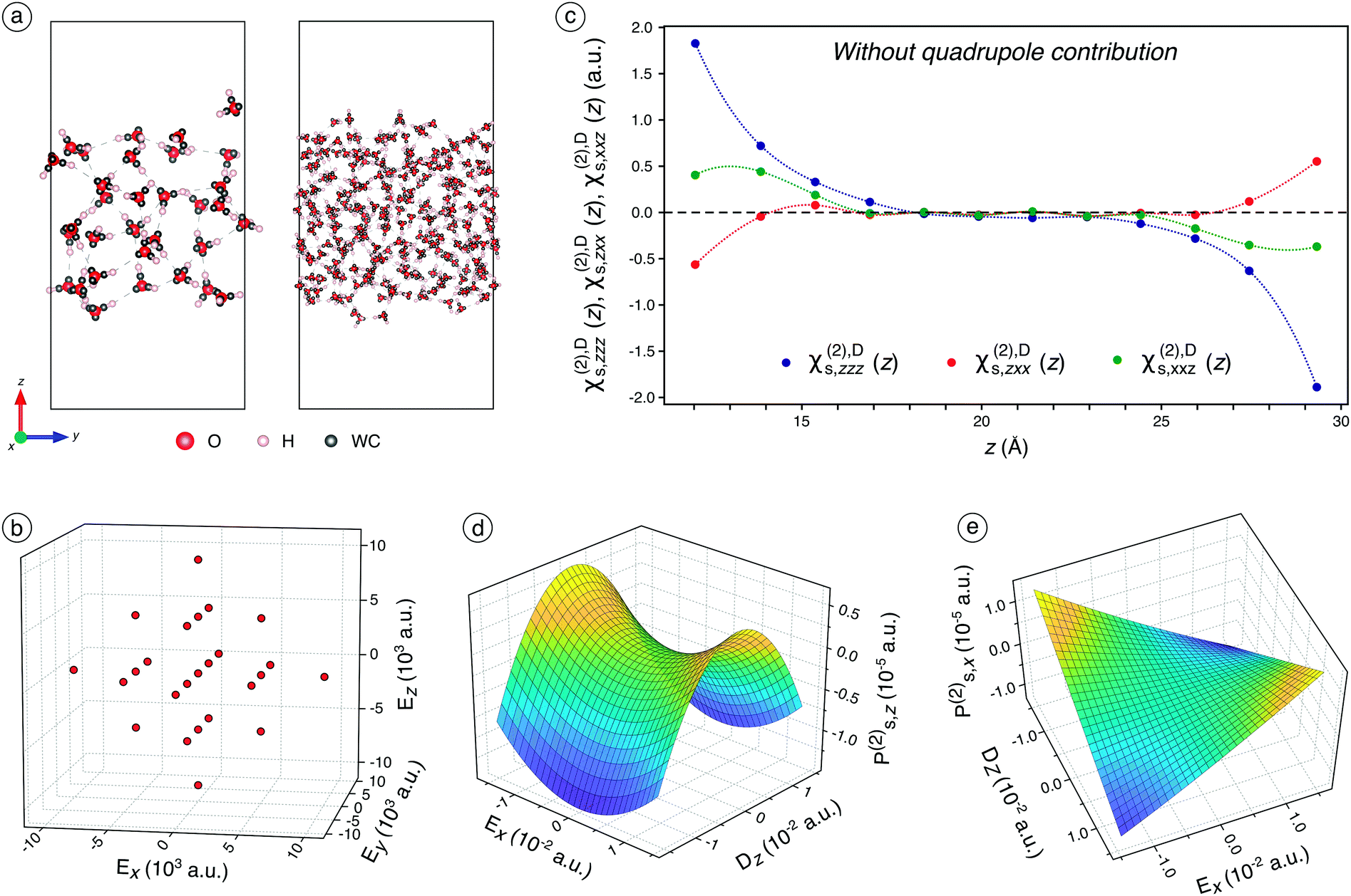

Fig. 1 (a) The two CMD simulation boxes used for the ab initio determination of χ_s,zzz⁽²⁾, χ_s,zxx⁽²⁾, and χ_s,xxz⁽²⁾; WC = Wannier centers. (b) 3D representation of the 25 external electric fields applied on each snapshot of the CMD simulation trajectory. (c) The dipole component of χ_s,zzz⁽²⁾, χ_s,zxx⁽²⁾, and χ_s,xxz⁽²⁾ calculated on slices of the water slab along the z-axis for the system containing 240 water molecules. (d) P_s,z⁽²⁾ as a function of E_x and D_z, without the inclusion of the bulk quadrupole contribution. (e) P_s,x⁽²⁾ as a function of E_x and D_z, without the inclusion of the bulk quadrupole contribution.

The dipole contribution to the SHG signal

Each point of Fig. 1c corresponds to 20 water molecules, which roughly represent half a layer. Only χ_s,zzz^(2),D, χ_s,zxx^(2),D, and χ_s,xxz^(2),D are non-zero and independent (the x ↔ y symmetry is respected), which is consistent with the SHG formalism for a water/air interface.^2–4,11 Those three components are significant only for between 1 and 2 layers of water molecules at the interface, before being zero in the bulk of water. This is consistent with the high interface-specificity of SHG since only the interfacial region displays a non-zero signal. Interestingly, when only the dipole contribution is considered, χ_s,zzz^(2),D and χ_s,xxz^(2),D are negative while χ_s,zxx^(2),D is positive. When whole slab halves are considered, P_s,z⁽²⁾ displays a significant concavity along D_z and a slight convexity along E_x (Fig. 1d). This illustrates the nonlinear dependence of P_s,z to the electric field (or displacement) components in two different ways: the quadratic concave behaviour along D_z indicates a negative χ_s,zzz^(2),D while the quadratic convex behaviour along E_x is attributed to a positive χ_s,zxx^(2),D, which is consistent with the trends observed in Fig. 1c. Meanwhile, E_x and D_z do not interact since the quadratic concave behaviour along D_z remains constant regardless of the value of E_x and vice versa. Thus, the interaction parameter, χ_s,zxz^(2),D, is not significant, which is consistent with the physical formalism of SHG.

Besides, P_s,x⁽²⁾ displays a typical negative interaction between E_x and D_z, which indicates a negative χ_s,xxz⁽²⁾ term (Fig. 1e), in agreement with Fig. 1c observation. Indeed, for E_x = 0, P_s,x⁽²⁾ remains constant around zero regardless of the value of D_z and vice versa while P_s,x⁽²⁾ increased or decreased significantly when both E_x and D_z increased in absolute value. Overall, according to Fig. 1c–e, one of the two calculated ratios is negative due to the negative χ_s,xxz⁽²⁾ and the positive χ_s,zxx⁽²⁾ components (all the fitted components of χ⁽¹⁾_s and χ_s⁽²⁾ are reported and discussed in Table S3† and associated text), which is inconsistent with our experimental values and with the values reported in the literature (reported in Table S2†). This unsound negative ratio is obtained whatever the cell sizes (32 and 240 molecules) and for various exchange-correlation functionals, with and without prior geometry optimisation, and for a high number of considered snapshots.

Adding the bulk quadrupole contribution

Considering the failure of sole dipole terms to predict an appropriate χ_s⁽²⁾, we then include the quadrupole contribution in the surface polarisation for the fitting procedure (see eqn (S25) to (S31)† and associated text). The fitted components of χ_s⁽¹⁾ and χ_s⁽²⁾ including quadrupole contribution are given in Table S3† while the influence of the number of molecules considered in the bulk quadrupole on the ratios is assessed and discussed in Fig. S13† and associated text.

When this is applied, χ_s,zzz⁽²⁾, χ_s,zxx⁽²⁾, and χ_s,xxz⁽²⁾ are still the only non-zero independent components of χ_s⁽²⁾, which is still in accordance with the SHG formalism. Besides, the behaviour of P_s,z⁽²⁾ changes significantly (Fig. 2a) while that of P_s,x⁽²⁾ remains roughly similar (Fig. 2b) compared to the previous case (Fig. 1d and e). The convexity observed for P_s,z⁽²⁾ is now transformed into a concavity, which indicates that χ_s,zxx⁽²⁾ becomes negative. The inclusion of the bulk quadrupole moments therefore induces a change of sign for one of the three non-zero components of χ_s⁽²⁾, which is of paramount importance for an optimal simulation of the SHG signal: since all the non-zero components of χ_s⁽²⁾ are now negative in our calculations, the two studied ratios are positive. The negativity of the three non-zero components of χ_s⁽²⁾ is in accordance with the reported assumptions^37,38 while the positiveness of the two ratios is in agreement with the experimental values, measured in this work and reported in the literature (see Table S2†).^39–46 Moreover, when the bulk quadrupole contribution is included, the permanent polarisation term along the z-axis, P_s,z⁽⁰⁾, represents an inner potential of −4.0991 V (see Table S3†), which is in very good agreement with the value of −3.87 V calculated by Remsing and co-workers⁴⁷ using DFT and with the value of −4.48 V determined experimentally by Yesibolati and co-workers.⁴⁸P_s,z⁽⁰⁾ is already non-zero when the dipole contribution only is considered but leads to a correct inner electric potential of water at the air/water interface only when the bulk quadrupole contribution is included.

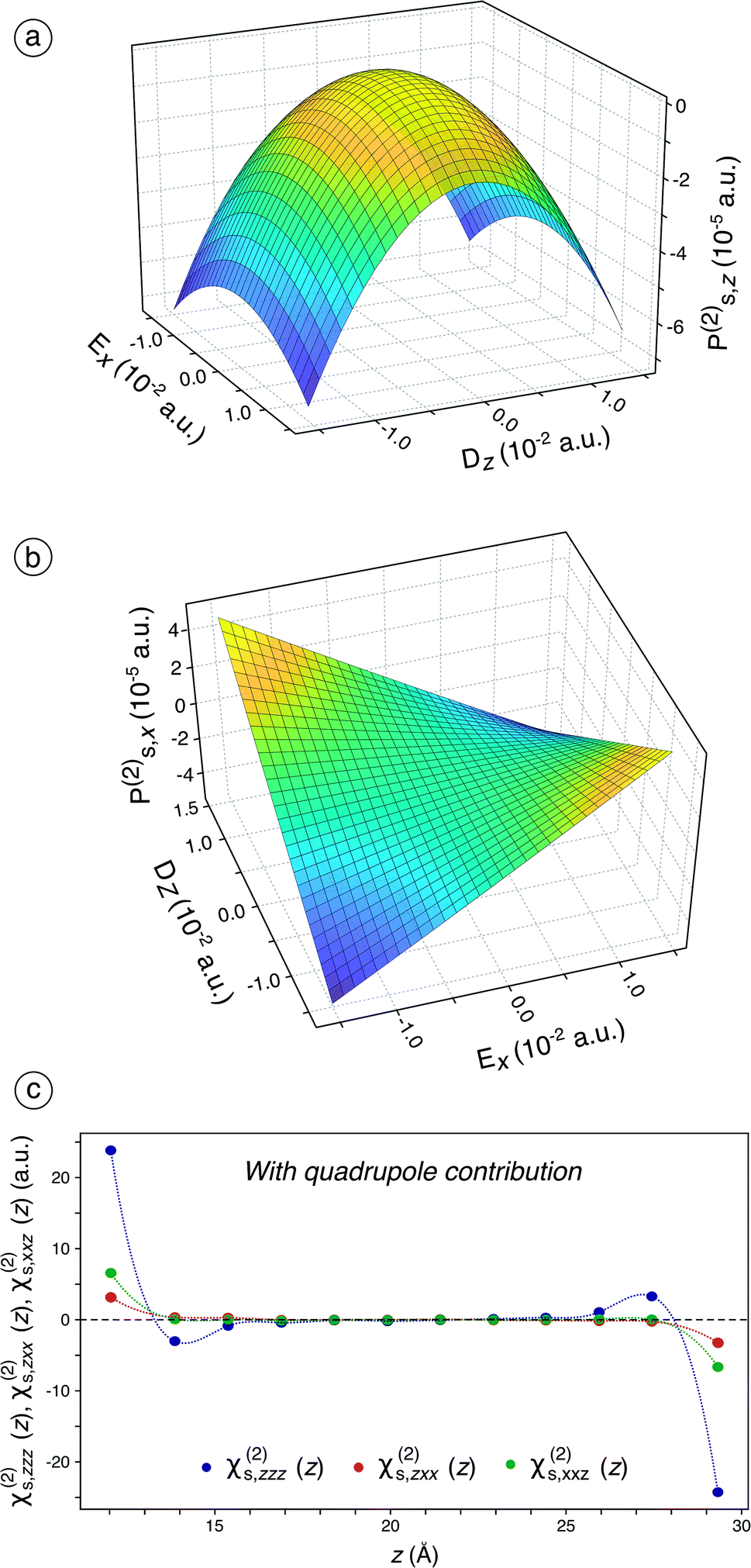Fig. 2 (a) P_s,z⁽²⁾ as a function of E_x and D_z, calculated using χ_s,zzz⁽²⁾, χ_s,zxx⁽²⁾, and χ_s,xxz⁽²⁾ determined on 144 snapshots of the system comprising 240 water molecules, with the inclusion of the bulk quadrupole contribution. (b) P_s,x⁽²⁾ as a function of E_x and D_z, calculated using χ_s,zzz⁽²⁾, χ_s,zxx⁽²⁾, and χ_s,xxz⁽²⁾ determined on 144 snapshots of the system comprising 240 water molecules, with the inclusion of the bulk quadrupole contribution. (c) Evolution of χ_s,zzz⁽²⁾, χ_s,zxx⁽²⁾, and χ_s,xxz⁽²⁾ that include the bulk quadrupole contribution calculated on slices of the water slab along the z-axis for the system containing 240 water molecules, averaged on 144 snapshots. Each slice comprises 20 water molecules, which roughly corresponds to half a layer.

A further crucial point in including the bulk quadrupole in the SHG signal definition is the invariance with respect to the choice of molecular centers. On the one hand, the quadrupole moment of a dipolar molecule depends on the defined molecular center. On the other hand, changing the molecular center affects the selection of molecules that belongs to one or the other interface, depending on their orientation. This induces a change of the interface dipole that is compensated by the change in molecular quadrupole moments. In Fig. S13† and associated text, we show that this invariance is nearly perfect for the z component of the interface polarisation. Recent developments in the modern theory of polarisation demonstrate that this is even true for changes of the electronic gauge.²³ This gauge invariance is not exact for the components of the polarisation parallel to the interface because of the truncation of the multipole expansion but numerical results in Fig. S13† show that higher order terms have negligible effect.

Interestingly, the bulk quadrupole contribution in the total surface polarisation is significantly higher than the interface dipole contribution. When only the dipole term is considered in the surface polarisation, P_s,z⁽²⁾ varies from −1.25 to 0.5 × 10⁻⁵ a.u. (Fig. 1d) while it varies from −7 to 0.5 × 10⁻⁵ a.u when this latter is included (Fig. 2a). Likewise, P_s,x⁽²⁾ varies from −1.0 to 1.0 × 10⁻⁵ a.u. on the whole E_x and D_z ranges when the bulk quadrupole contribution is not included (Fig. 1e) while it varies from −4.0 to 4.0 × 10⁻⁵ a.u on the same ranges when the quadrupole contribution is included (Fig. 2b). Hence, the bulk quadrupole contribution is several times higher than the interface dipole contribution and it largely dominates the simulated SHG signal for a water/air interface. The importance of the bulk quadrupole contribution had been previously suggested theoretically^37,38 and is here demonstrated through direct ab initio determination of the surface dipole response. We will in the next section analyse further how the electronic response induces a surface dipole through this bulk quadrupole contribution.

When the fitting is performed on slices along the z-axis (Fig. 2c), the results previously observed in Fig. 2a and b are confirmed, i.e., all the three components of χ_s⁽²⁾ are now negative. Only the half molecular layer closest to the vacuum phase exhibits non-zero χ_s,zxx⁽²⁾ and χ_s,xxz⁽²⁾. It turns out that the interface-specificity of SHG is increased when the bulk quadrupole term is included. Besides, χ_s,zzz⁽²⁾ is significant and negative for the half layer closest to the vacuum phase but becomes slightly positive for more-buried water molecules, which probably originates from the decrease of the electron density just inside the interface.

The bulk quadrupole from an electronic point of view

From an electronic point of view, the quadrupole contribution represents the overspill of electrons from the interface into the vacuum. Regardless of the orientation of the molecules at the interface and under the zero field, electrons are systematically first encountered when crossing the interface. This induces a negative local charge just outside the Gibbs interface and, therefore, a positive local charge inside the Gibbs interface. This results in the existence of the aforementioned non-zero (negative) permanent surface polarisation that corresponds to an inner electric potential of −4.0991 V. This non-zero permanent surface potential does not arise from the presence of charges – since we did not include any – but rather to the slight separation of the positive and negative charges at the interface, as presented in Fig. 3b. Upon application of an external electric field, we observe the dilatation of the electron density around each atom of the water molecules in the slab, as calculated in Fig. 3a. This results in an exacerbated electron overspill in the vacuum as shown in Fig. 3b. The dipole response of the bulk is zero however since it depends on (1) the orientation of molecules, which is random in the bulk, and on (2) the gradient of the quadrupole moments, which is only significant at the interface.

Fig. 3 (a) Charge density over a cross-section of an oxygen atom. (b) Charge density integrated on small slices over the z-axis. Blue = positive charge; red = negative charge; dashed red = negative charge under the zero field; full red = negative charge under an electric field of 10 a.u.; green = difference between the total charge densities under the two fields. (c) Schematic effect of an electric field on water molecules of a water/air interface, (d) with a global charge density point of view, (e) and by displaying only the second-order variations of the charge density. Yellow = positive, blue = negative. In all sub-figures, the black dashed line represents the Gibbs interface.

The surface dipole moment becomes more negative due to a higher decoupling of the negative and positive charges in atoms (Fig. 3b). The dilatation of the electron density occurs for all atoms in the water slab, as schematically represented in Fig. 3c. However, because of the uniform distribution of molecules, it does not lead to any signal in the bulk. The application of an electric field, due to the increase of the width of the electron clouds, results in a decrease of the quadrupole moments, which become more negative, and therefore induces a decrease of the surface dipole moment, which also becomes more negative. The electronic interface is shifted towards the vacuum phase due to the dilation of the electron clouds as represented in Fig. 3d, while the Gibbs interface, representing the interface under a nuclear point of view, does not move. This is confirmed by the second-order variations of the electron density calculated on our systems with or without an applied electric field (Fig. 3e): positive variations (i.e., higher electron densities) are displayed outside the Gibbs interface, which perfectly highlights the decrease of the surface dipole moment. On overall, the bulk quadrupole moments can be seen as the convolution of the function describing the distribution of atomic layers by the width of the electron clouds. Therefore, the increase of the electron clouds width induces more negative quadrupole moments.

Predicting SHG signals

When the bulk quadrupole contribution is included, we obtain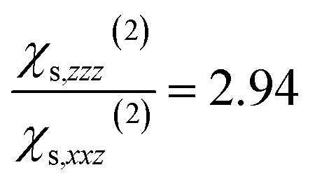 and 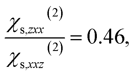calculated on 144 snapshots for the system comprising 240 water molecules. These values are close to our experimental values of 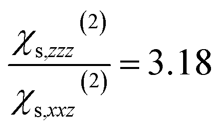and 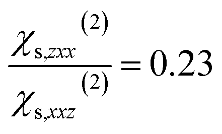and to the average of all the experimental values reported in the literature (see Table S2† and associated text for its determination) of 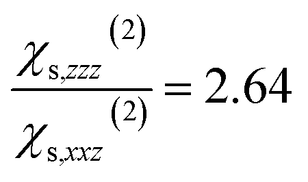and Since significant variations of the two considered ratios are not necessarily related to important variations of the SHG responses (see Fig. S7†), we compare only the SHG responses (experimental and simulated) in terms of normalised intensities and errors committed on them.

As presented in Fig. 4, our SHG simulated signal is in very good agreement with our experimental results, which validates this method and demonstrates its strength. Our simulations are conducted on pure water while, in reality, the experimental system is not pure because of the equilibrium with CO₂ of the atmosphere. However, the proportionality factor, ψ₀, controlling the contribution of ions is zero at pH higher than 3 and, therefore, also at pH 5.8.⁴⁹ At those pH, χ⁽²⁾ is identified to the sole contribution of the neat surface, which makes possible the comparison of our calculations with experimental results for a real surface. The root-mean-square error (RMSE) between our simulated and our experimental SHG responses are 0.0501, 0.0138, and 0.0440 for the P-polarised, S-polarised, and 45°-polarised curves, respectively (in arbitrary normalized units). These values are of the same order of magnitude than the RMSE between various SHG responses reported in the literature and the SHG experiments from this work, as presented in Fig. S7.† Moreover, the mean absolute percentage error, which corresponds to the average error committed on the prediction of the SHG intensities expressed as a percentage of the experimental value, are 4.47%, 1.13%, and 2.92% for the P-polarised, S-polarised, and 45°-polarised curves, respectively. This means that our ab initio predictions estimate the experimental values with less than 5% error. Besides, a limited number of snapshots is required to obtain a satisfactory accuracy on the two ratios, which constitutes a key point of this method: for the system containing 240 water molecules, 13 snapshots allowed reaching the 95% confidence interval located around the average value (calculated on 144 snapshots) for the two ratios, respectively (see Fig. S10 and S11† and associated text). BLYP exchange-correlation functional provides results with satisfactory accuracy compared to other functionals, including hybrid ones, while an eventual geometry optimisation, performed prior the relaxation of the wavefunctions under an applied electric field, does not affect significantly the prediction of the ratios and can therefore be avoided (see Table S4† and associated discussions). The considered snapshots are extracted from CMD simulations, in which the O–H intra-molecular bond length is roughly and approximately set constant to 1 Å. Since the geometry optimisation does not influence the prediction of SHG responses, those latter therefore lowly depend on intra-molecular forces and mostly on the inter-molecular interactions, i.e., hydrogen bonds, which are generally accurately described using CMD simulations. On overall, the agreement with the experimental SHG signal of a water/air interface demonstrates that considering higher order terms such as the third-order terms or the octupole contributions is not required and that those terms are probably negligible in the total response.

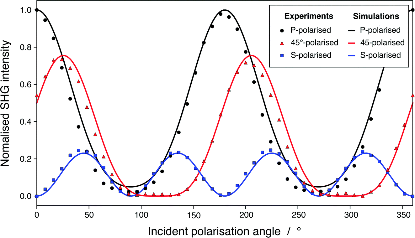Fig. 4 P-(black), S-(blue), and 45°-polarised (red) experimental SHG responses for a water/air interface (points) and simulated SHG responses (lines) plotted using χ_s,zzz⁽²⁾, χ_s,zxx⁽²⁾, and χ_s,xxz⁽²⁾ calculated using the direct ab initio method developed here.

The high dependency of the SHG response to the local environment of molecules partly explains the difficulty to simulate SHG signals using the molecular hyperpolarisability, β. Indeed, from a molecule in vacuo to a molecule in an ice-like configuration, two of the three non-zero independent components of β change their sign and significantly their absolute value (Fig. S1†), which is in accordance with several works reported in the literature.^27–30 This influence of the environment is not limited to water molecules since previous works on molecular crystals and thin films highlighted significant changes of the hyperpolarisability due to the local polarisation originating from the surrounding molecules and to the dynamical structural flexibility of the considered organic molecules.^50,51 Moreover, the influence of the environment is not reduced to the application of a local field in response to the applied field. Indeed, Mikkelsen and co-workers²⁷ demonstrated that the presence of an explicit solvation shell, with explicit hydrogen bonds, is required to observe this change of sign while simply applying a dielectric medium having the dielectric properties of water does not result in such sign inversion. These results are consistent with our calculation of the dipolar contribution to the SHG signal but highlight the strong role played by hydrogen bonds in the SHG signal and the strong dependency of this latter to the local environment. This underlines the need for global models that are freed from local concepts, both in terms of the molecular polarisation response and of the edge polarisation that includes a non-local quadrupole contribution, as the method presented here.

Discussion and conclusion

Overall, the direct ab intio method developed here allows highlighting the large dominance of the SHG signal by the bulk quadrupole contribution, which completely overwhelms the interface dipole term for a water/air interface. Therefore, the SHG experiments are only slightly sensitive to the orientation of the molecules at the interface since the signal mostly relies on the bulk quadrupole term, which does not depend, by definition, upon the molecular orientation. However, this assertion has to be balanced since the bulk quadrupole contribution is proportional to the difference of electron densities or dielectric permittivities between the two media, in accordance with the literature.^20,21,37,52 This difference is maximal in the case of a water/air interface, which explains the overwhelming bulk quadrupole contribution. Hence, in the case of an interface between two liquids presenting closer dielectric permittivities, the dipole and quadrupole contributions could be of the same order of magnitude. Nevertheless, for an accurate prediction of a SHG response, the bulk quadrupole terms should inevitably be included in the calculations; the interpretation of the SHG experimental signal at a molecular level should also consider their significance, which ineluctably decreases the dependence of the SHG response to the orientation of the molecules at the interface. The interfacial dipole signal could however be magnified in experiments by artificially removing the bulk quadrupole contribution: when one investigates an interfacial process, the bulk quadrupole contribution should not vary significantly and, therefore, recording a blank signal could allow isolating the interfacial dipole term and its variation over the interfacial process. Besides, our method can be easily transferred and applied to other systems, including other types of interfaces, organic molecules, or charged species. However, this transfer could require some adaptations and modifications in the method since, as instance, for solid/liquid interfaces with a non-zero ionic strength, authors recently introduced a new imaginary third-order term to determine a sound χ⁽²⁾.^49,53,54 Finally, the simulation and interpretation of the SHG signal cannot rely on a local hyperpolarisability: the effects due to the permanent (local and non-local) electric fields are crucial for the simulation of SHG signals, as it has been demonstrated in previous works.^{49–51,53,54} Similarly to polarisability, the hyperpolarisability depends upon the local chemical environment of the molecules, but unlike the polarisability, the environment does not only change the amplitude, it also changes its sign. As a result, in condensed phase, the use of the concept of an effective molecular hyperpolarisability is only possible by finely characterising its dependence on the local chemical environment of the water molecules, particularly in terms of number and length(s) of hydrogen bonds. This work paves the way to a new consideration of SHG interpretation and understanding and may stimulate further research in this field, in particular to develop new models based on the local hyperpolarisability.

Methods

SHG experiments

The SHG apparatus used in our study was based on a femtosecond Ti-sapphire oscillator laser source that provided 100 fs pulses at a repetition rate of 80 MHz (Spectra-Physics, model Mai Tai). A low-pass filter was placed between the laser and the interface to remove any unwanted harmonic light in the incident beam. The fundamental beam, at a wavelength of 800 nm and an average power of 3 W, was then focused on the water/air interface by a 10 cm-focal lens. To obtain this interface, a Petri dish was filled with water and placed on the optical path so that the incidence angle was 70°. After the interface, the reflected beam was focused by a 10 cm-focal lens and passed through a high-pass filter to remove the fundamental photons (at a wavelength of 800 nm) and only select the second harmonic light, at a wavelength of 400 nm. The second harmonic light was then detected and counted using a Princeton Instruments Acton SP-2358 Czerny-Turner grating (300 grooves per mm with a 500 nm blaze angle) spectrometer, with a PIXIS 400B backilluminated thermoelectrically-cooled CCD detector.

This setup was optimised to cover the wavelength range 300–600 nm. The incident beam was linearly polarised using a rotation half-wave plate. The incident polarisation angle varied from 0° to 360° with a measurement every 8°. The S- and P-polarised second harmonic intensities were selected using an analyser, consisting of a half-wave plate combined with a Glan-Thompson Calcite polariser, placed on the optical path of the reflected beam, in front of the spectrometer. Ultrapure water (Milli-Q Labo, Millipore) was used for the experiments. χ_s,zzz⁽²⁾, χ_s,zxx⁽²⁾, χ_s,xxz⁽²⁾ were fitted by the least-squares method using a Levenburg–Marquardt gradient for the minimisation.^55,56 The fitting was carried out on eqn (S1)–(S3)† using the measured intensities as the y-values and the corresponding incident polarisation angles as the x-values.

Molecular dynamics simulations

Simulation boxes of 1 × 1 × 1 nm and 2 × 2 × 2 nm were created and filled with water molecules using the packmol software.⁵⁷ The boxes contained 32 and 240 water molecules, respectively, which roughly corresponded to a density of 1 g cm⁻³. An NPT simulation at T = 298.15 K and P = 1.01325 bar was conducted on each box during 1 ns to reach the equilibrium. Then, the cell dimension was doubled along the z-axis to create a water/air interface on which an NVT simulation at T = 298.15 K was performed during 10 ns, for each simulation box. The 3-site rigid SPC/E model⁵⁸ was used to describe water molecules, considering the satisfactory performances of this model to reproduce the structure and properties of water at ambient conditions.^58–61 Besides, the inter-molecular interactions were described using a Coulomb and a 12–6 Lennard-Jones potentials. According to the SPC/E model, σ = 3.166 Å and ε = 78.197 K for the oxygen atom while both were zero for the hydrogen atom.⁵⁸ A SHAKE algorithm⁶² was used to constrain water molecular geometry with a tolerance of 10⁻⁴.

The molecular dynamics simulations were performed with the open Large-scale Atomic/Molecular Massively Parallel Simulator (LAMMPS) package⁶³ with periodic boundary conditions upon the three directions. A cut-off distance of 10 Å was applied to calculate the non-bonded potential energies while the long-range electrostatic interactions were computed using the particle–particle particle-mesh (PPPM) solver⁶⁴ with an accuracy value of 10⁻⁴. The equations of motion were solved using the velocity-Verlet integrator with a time-step of 1 fs, under a Nose/Hoover thermostat and barostat (for NPT simulations).^65,66 During the simulation, one snapshot was recorded every 1 ps for the quantum mechanical calculations.

Quantum mechanics calculations

Density functional theory (DFT) calculations were performed using the Car Parrinello Molecular Dynamics (CPMD) package.⁶⁷ The Becke, Lee, Yang, and Parr (BLYP) functional^68,69 in the generalized gradient approximation⁷⁰ was employed for the exchange-correlation term. Since only the valence electrons were considered, norm-conserving Troullier–Martins pseudo-potentials⁷¹ were used in the plane-wave basis set, with an energy cutoff of 150 Rydberg. Considering the large size and disorder of the cell, the calculations were realised at the γ-point of the Brillouin zone only. The method of direct inversion in the iterative subspace (DIIS)⁷² was used for the wave function optimisation and combined with a quasi-Newton method⁷³ for the ionic positions relaxation, when this was carried out. In such cases, to help the optimisation of the ionic positions, the initial approximate Hessian was constructed based on a unit matrix and the limited-memory BFGS method was used.⁷⁴ For the structural and wave function optimisations, convergence criteria of 5 × 10⁻⁴ and 10⁻⁵ were applied, respectively. The atoms, Wannier centers, and electron densities were all visualised using the VESTA software.⁷⁵ For further details about the method used for determining the second-order electric susceptibility, please report to Fig. S2† and associated text.

Author contributions

R. V., J.-F. D. and Y. F. planned the study and derived the formalism. Y. F. performed the simulations and numerical data analysis. O. D. and A. J. carried out the SHG experiments. Y. F., J.-F. D., and R. V. wrote the main paper and methods information. B. S., J.-F. D., R. V., M. D., and Y. F. regularly discussed the results. All authors commented on the manuscript at each stage.

Conflicts of interest

There are no conflicts to declare.

Acknowledgements

The authors thank the CEA program SHG Future and the RCHIM structure for their financial support. This work was granted access to the HPC resources of TGCC under the allocation 2020-A0080911513 made by GENCI.

Notes and references

1. P. A. Franken, A. E. Hill, C. W. Peters and G. Weinreich, Phys. Rev. Lett., 1961, 7, 118–119.
2. Y. R. Shen, Nature, 1989, 337, 519–525.
3. K. B. Eisenthal, Chem. Rev., 1996, 96, 1343–1360.
4. R. M. Corn and D. A. Higgins, Chem. Rev., 1994, 94, 107–125.
5. B. Pozniak and D. A. Scherson, J. Am. Chem. Soc., 2003, 125, 7488–7489.
6. G. C. Gschwend, A. Olaya and H. H. Girault, Chem. Sci., 2020, 11, 10807–10813.
7. C. Macias-Romero, I. Nahalka, H. I. Okur and S. Roke, Science, 2017, 357, 784–788.
8. D. Neshev and Y. Kivshar, Science, 2014, 344, 483–484.
9. E. De Meulenaere, W.-Q. Chen, S. Van Cleuvenbergen, M.-L. Zheng, S. Psilodimitrakopoulos, R. Paesen, J.-M. Taymans, M. Ameloot, J. Vanderleyden, P. Loza-Alvarez, X.-M. Duan and K. Clays, Chem. Sci., 2012, 3, 984.
10. A. C. McGeachy, E. R. Caudill, D. Liang, Q. Cui, J. A. Pedersen and F. Geiger, Chem. Sci., 2018, 9, 4285–4298.
11. R. W. Boyd, Nonlinear Optics, Academic Press Inc, Amsterdam ; Boston, 3rd edn, 2008.
12. Y. R. Shen, Annu. Rev. Phys. Chem., 1989, 40, 327–350.
13. G. Martin-Gassin, P. M. Gassin, L. Couston, O. Diat, E. Benichou and P. F. Brevet, Phys. Chem. Chem. Phys., 2011, 13, 19580.
14. F. C. Boman, M. J. Musorrafiti, J. M. Gibbs, B. R. Stepp, A. M. Salazar, S. T. Nguyen and F. M. Geiger, J. Am. Chem. Soc., 2005, 127, 15368–15369.
15. S. S. Jha, Phys. Rev. Lett., 1965, 15, 412–414.
16. S. S. Jha, Phys. Rev., 1965, 140, A2020–A2030.
17. S. S. Jha and C. S. Warke, Phys. Rev., 1967, 153, 751–759.
18. N. Bloembergen, R. K. Chang, S. S. Jha and C. H. Lee, Phys. Rev., 1968, 174, 813–822.
19. J. Rudnick and E. A. Stern, Phys. Rev. B, 1971, 4, 4274–4290.
20. P. Guyot-Sionnest, W. Chen and Y. R. Shen, Phys. Rev. B, 1986, 33, 8254–8263.
21. P. Guyot-Sionnest and Y. R. Shen, Phys. Rev. B, 1987, 35, 4420–4426.
22. I. López-Duarte, J. E. Reeve, J. Pérez-Moreno, I. Boczarow, G. Depotter, J. Fleischhauer, K. Clays and H. L. Anderson, Chem. Sci., 2013, 4, 2024.
23. S. Ren, I. Souza and D. Vanderbilt, Phys. Rev. B, 2021, 103, 035147.
24. N. Bloembergen and P. S. Pershan, Phys. Rev., 1962, 128, 606–622.
25. J. Ducuing and N. Bloembergen, Phys. Rev. Lett., 1963, 10, 474–476.
26. P. Guyot-Sionnest and Y. R. Shen, Phys. Rev. B, 1988, 38, 7985–7989.
27. K. V. Mikkelsen, Y. Luo, H. Ågren and P. Jo/rgensen, J. Chem. Phys., 1995, 102, 9362–9367.
28. P. Kaatz, E. A. Donley and D. P. Shelton, J. Chem. Phys., 1998, 108, 849–856.
29. A. V. Gubskaya and P. G. Kusalik, Mol. Phys., 2001, 99, 1107–1120.
30. C. Liang, G. Tocci, D. M. Wilkins, A. Grisafi, S. Roke and M. Ceriotti, Phys. Rev. B, 2017, 96, 041407.
31. G. H. Wannier, Phys. Rev., 1937, 52, 191–197.
32. N. Marzari and D. Vanderbilt, Phys. Rev. B, 1997, 56, 12847–12865.
33. N. Marzari, A. A. Mostofi, J. R. Yates, I. Souza and D. Vanderbilt, Rev. Mod. Phys., 2012, 84, 1419–1475.
34. R. Resta, Europhys. Lett., 1993, 22, 133–138.
35. D. Vanderbilt and R. D. King-Smith, Phys. Rev. B, 1993, 48, 4442–4455.
36. R. D. King-Smith and D. Vanderbilt, Phys. Rev. B, 1993, 47, 1651–1654.
37. K. Shiratori, S. Yamaguchi, T. Tahara and A. Morita, J. Chem. Phys., 2013, 138, 064704.
38. S. Yamaguchi, K. Shiratori, A. Morita and T. Tahara, J. Chem. Phys., 2011, 134, 184705.
39. A. J. Fordyce, W. J. Bullock, A. J. Timson, S. Haslam, R. D. Spencer-Smith, A. Alexander and J. G. Frey, Mol. Phys., 2001, 99, 677–687.
40. W.-k. Zhang, D.-s. Zheng, Y.-y. Xu, H.-t. Bian, Y. Guo and H.-f. Wang, J. Chem. Phys., 2005, 123, 224713.
41. T. T. Pham, A. Jonchère, J.-F. Dufrêche, P.-F. Brevet and O. Diat, J. Chem. Phys., 2017, 146, 144701.
42. Q. Wei, D. Zhou and H. Bian, Phys. Chem. Chem. Phys., 2018, 20, 11758–11767.
43. A. A. T. Luca, P. Hébert, P. F. Brevet and H. H. Girault, J. Chem. Soc., Faraday Trans., 1995, 91, 1763–1768.
44. H.-t. Bian, R.-r. Feng, Y.-y. Xu, Y. Guo and H.-f. Wang, Phys. Chem. Chem. Phys., 2008, 10, 4920.
45. H.-t. Bian, R.-r. Feng, Y. Guo and H.-f. Wang, J. Chem. Phys., 2009, 130, 134709.
46. M. C. Goh, J. M. Hicks, K. Kemnitz, G. R. Pinto, T. F. Heinz, K. B. Eisenthal and K. Bhattacharyya, J. Phys. Chem., 1988, 92, 5074–5075.
47. R. C. Remsing, M. D. Baer, G. K. Schenter, C. J. Mundy and J. D. Weeks, J. Phys. Chem. Lett., 2014, 5, 2767–2774.
48. M. N. Yesibolati, S. Laganà, H. Sun, M. Beleggia, S. M. Kathmann, T. Kasama and K. Mølhave, Phys. Rev. Lett., 2020, 124, 065502.
49. L. Dalstein, K.-Y. Chiang and Y.-C. Wen, J. Phys. Chem. Lett., 2019, 10, 5200–5205.
50. C. Bouquiaux, C. Tonnelé, F. Castet and B. Champagne, J. Phys. Chem. B, 2020, 124, 2101–2109.
51. T. Seidler, A. Krawczuk, B. Champagne and K. Stadnicka, J. Phys. Chem. C, 2016, 120, 4481–4494.
52. K. Shiratori and A. Morita, Bull. Chem. Soc. Jpn., 2012, 85, 1061–1076.
53. E. Ma, P. E. Ohno, J. Kim, Y. Liu, E. H. Lozier, T. F. Miller, H.-F. Wang and F. M. Geiger, J. Phys. Chem. Lett., 2021, 12, 5649–5659.
54. E. Ma, J. Kim, H. Chang, P. E. Ohno, R. J. Jodts, T. F. Miller and F. M. Geiger, J. Phys. Chem. C, 2021, 125, 18002–18014.
55. K. LEVENBERG, Q. Appl. Math., 1944, 2, 164–168.
56. D. W. Marquardt, J. Soc. Ind. Appl. Math., 1963, 11, 431–441.
57. L. Martínez, R. Andrade, E. G. Birgin and J. M. Martínez, J. Comput. Chem., 2009, 30, 2157–2164.
58. H. J. C. Berendsen, J. R. Grigera and T. P. Straatsma, J. Phys. Chem., 1987, 91, 6269–6271.
59. Y. Wu, H. L. Tepper and G. A. Voth, J. Chem. Phys., 2006, 124, 024503.
60. P. G. Kusalik and I. M. Svishchev, Science, 1994, 265, 1219–1221.
61. M. W. Mahoney and W. L. Jorgensen, J. Chem. Phys., 2000, 114, 363–366.
62. J.-P. Ryckaert, G. Ciccotti and H. J. C. Berendsen, J. Comput. Phys., 1977, 23, 327–341.
63. S. Plimpton, J. Comput. Phys., 1995, 117, 1–19.
64. R. W. Hockney and J. W. Eastwood, Computer simulation using particles, A. Hilger, Bristol ; Philadelphia, 1988.
65. S. Nosé, J. Chem. Phys., 1984, 81, 511–519.
66. W. G. Hoover, Phys. Rev. A, 1985, 31, 1695–1697.
67. CPMD, http://www.cpmd.org/, copyright IBM Corp 1990-2008, copyright MPI für Festkörperforschung Stuttgart, 1997–2001.
68. C. Lee, W. Yang and R. G. Parr, Phys. Rev. B, 1988, 37, 785–789.
69. A. D. Becke, Phys. Rev. A, 1988, 38, 3098–3100.
70. J. P. Perdew, K. Burke and M. Ernzerhof, Phys. Rev. Lett., 1996, 77, 3865–3868.
71. N. Troullier and J. L. Martins, Phys. Rev. B, 1991, 43, 1993–2006.
72. J. Hutter, H. P. Lüthi and M. Parrinello, Comput. Mater. Sci., 1994, 2, 244–248.
73. P. Császár and P. Pulay, J. Mol. Struct., 1984, 114, 31–34.
74. C. Grossmann, Z. Angew. Math. Mech., 1981, 61, 408.
75. K. Momma and F. Izumi, J. Appl. Crystallogr., 2008, 41, 653–658.

---

Footnote

† Electronic supplementary information (ESI) available. See DOI: 10.1039/d1sc03960a

---