DOI:
10.1039/D2RA06433B
(Paper)
RSC Adv., 2022,
12, 33479-33487
DLBLS_SS: protein secondary structure prediction using deep learning and broad learning system
Received
12th October 2022
, Accepted 16th November 2022
First published on 23rd November 2022
Abstract
Protein secondary structure prediction (PSSP) is not only beneficial to the study of protein structure and function but also to the development of drugs. As a challenging task in computational biology, experimental methods for PSSP are time-consuming and expensive. In this paper, we propose a novel PSSP model DLBLS_SS based on deep learning and broad learning system (BLS) to predict 3-state and 8-state secondary structure. We first use a bidirectional long short-term memory (BLSTM) network to extract global features in residue sequences. Then, our proposed SEBTCN based on temporal convolutional networks (TCN) and channel attention can capture bidirectional key long-range dependencies in sequences. We also use BLS to rapidly optimize fused features while further capturing local interactions between residues. We conduct extensive experiments on public test sets including CASP10, CASP11, CASP12, CASP13, CASP14 and CB513 to evaluate the performance of the model. Experimental results show that our model exhibits better 3-state and 8-state PSSP performance compared to five state-of-the-art models.
1 Introduction
As an important part of cell composition, proteins are not only the basis of life activities, but also play an important role in transporting substances, catalyzing chemical reactions and immune functions. The tertiary structure of a protein determines its function. However, existing techniques for predicting tertiary structure are time-consuming and expensive.1,2 Secondary structure is the spatial arrangement of atoms in the backbone of a peptide chain. The tertiary structure is formed by further folding on the basis of the secondary structure. Therefore, the study of protein secondary structure directly affects the prediction of tertiary structure.3,4 As an important task in bioinformatics, protein secondary structure prediction (PSSP) not only contributes to the study of protein function and structure but also facilitates the design and development of new drugs.
According to the division method of the DSSP program, the 8 states of protein secondary structure include G (helix), I (π-helix), H (α-helix), B (β-bridge), E (β-sheet), T (turn), S (bend) and C (coil).5 The 8-state protein secondary structure can also be classified into 3 states: H (helix), B (strand) and C (coil).6,7 In the early stages of research, machine learning methods such as support vector machines,8,9 K-nearest neighbors,10,11 and neural networks12,13 focused extensively on 3-state PSSP. However, the complex 8-state secondary structure has richer protein information and is more conducive to protein research.
In recent years, continuously developed and improved deep learning techniques have been widely used in PSSP, which exhibit superior performance and can improve computing speed. The PSIPRED14 method utilized two feedforward neural networks for PSSP. The JPred4 (ref. 15) method utilized the JNet algorithm to predict the secondary structure. The SSpro16 model used an ensemble of BRNN for prediction. The DeepCNF17 model utilized shallow neural networks and conditional neural fields to model the mapping relationship between features and labels. Zhou et al. introduced a convolutional architecture in a supervised generative stochastic network to improve PSSP.18 The SSREDNs3 model used deep recurrent encoder-decoder networks for PSSP. The SPIDER3 server utilized a deep model LSTM-BRNN for 3-state prediction.19 The SPOT-1D method utilized an ensemble model consisting of LSTM-BRNN and residual network for prediction.20 The NrtSurfP-2.0 model utilized CNN and BLSTM to extract local and global dependencies between amino acid residues.21 The SAINT method introduced a self-attention mechanism in the Deep3I network to extract secondary structure features.22 The OPUS-TASS method combined CNN, BLSTM and Transformer architectures to improve accuracy.23 The MLPRNN method used two MLP blocks and one BGRU to predict the secondary structure.24
Inspired by the application and effectiveness of deep learning in PSSP, we propose SETCN to extract key deep features in protein sequences by introducing Squeeze-and-Excitation25 (SE) blocks in temporal convolutional networks26 (TCN). Since secondary structure recognition is affected by residues in front and rear positions, we further propose SEBTCN to extract deep features bidirectionally.
To improve PSSP, we propose a novel prediction model DLBLS_SS for 3-state and 8-state PSSP based on bidirectional long short-term memory27 (BLSTM) network, SEBTCN and broad learning system28 (BLS). The input features of the model are position-specific scoring matrix (PSSM)29 profiles and one-hot encoding. In DLBLS_SS, BLSTM can extract global interactions in residue sequences, SEBTCN can capture bidirectional key long-range dependencies between residues, and BLS can further quickly extract local optimal features and complete classification.
The main contributions of this paper include: (1) we propose SETCN by introducing the channel attention mechanism SE block in TCN, which can extract key deep features in the sequence. (2) We further propose SEBTCN by improving SETCN, which can bidirectionally extract key deep features in sequences. (3) We propose a novel PSSP model using BLSTM, SETCN and BLS to improve feature extraction of residue sequences. To the best of our knowledge, this is the first application of BLS in PSSP. (4) Experimental results on seven benchmark datasets demonstrate that the proposed method achieves state-of-the-art performance compared to five popular methods.
2 Material and methods
2.1. Bidirectional long short-term memory networks (BLSTM)
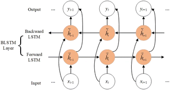
For long protein sequences, recurrent neural networks30 not only have inevitable error accumulation when transmitting useful information, but also may have problems such as exploding gradients. Therefore, we use BLSTM to capture the global features of the sequence, which can extract important information while automatically discarding useless information. As shown in Fig. 1, BLSTM contains forward LSTM and backward LSTM, which can obtain bidirectional interactions of sequences through forward and backward extraction of information. The computation of a standard LSTM31 cell at time t is as follows:| | |
it = σ(Wxi × xt + Whi × ht−1 + bi)
| (1) |
| | |
ft = σ(Wxf × xt + Whf × ht−1 + bf)
| (2) |
| | |
ot = σ(Wxo × xt + Who × ht−1 + bo)
| (3) |
| | |
ct = ft ⊙ ct−1 + it ⊙ tanh(Wxc × xt + Whc × ht−1 + bc)
| (4) |
where i is the input gate, f is the forget gate, o is the output gate, σ is the activation function, xt is the input, ht is the output, W is the weight, b is the bias, ct is the unit state, ☉ represents the element-wise multiplication, and tanh represents the hyperbolic tangent function.
 |
| | Fig. 1 The architecture of BLSTM. | |
2.2. The proposed SEBTCN
As a sequence-to-sequence prediction network, TCN has the characteristics of stable training, low memory requirements, flexible receptive field, and parallel computing. To enhance the ability to extract key features in residue sequences, we introduce a channel attention module in the TCN residual block. Furthermore, secondary structure recognition is not only affected by residues in past positions, so we further propose SEBTCN to capture bidirectional deep features between residues.
2.2.1. Dilated causal convolution. The network uses causal convolution to prevent the loss of future information, so the output at time t depends on the input at time t and historical time. However, for sequences that rely on long histories, the network requires extremely deep architectures or large filters, which brings huge computational workload.To expand the receptive field to obtain long historical information, the network introduces dilated convolutions. The computation of the dilated convolution F on the sequence element s is:
| |
 | (6) |
where
x is the input,
f and
k are the filter and filter size,
d is the dilation factor, and
s −
d·
i is the history direction. Since the dilation factor increases exponentially with the number of layers in the network (
d = 2
n at layer
n), the network has an extremely large receptive field and its top layers can get more information. The dilated causal convolution structure is shown in
Fig. 2(a).
 |
| | Fig. 2 Architecture in the network. (a) The dilated causal convolution. (b) The residual connection. | |
2.2.2. Residual connections. For high-dimensional sequences, the network may require extremely deep layers, but it is difficult to maintain stability during training. Therefore, as shown in Fig. 2(b), the network introduces residual connections, which operate on the input X as follows:| | |
O = activation(X + F(X))
| (7) |
where F is a series of transformations. Residual connections can allow each layer to learn to modify the identity map rather than all transformations, which is beneficial for very deep networks.
2.2.3. SETCN residual block. The architecture of the SETCN residual block is shown in Fig. 3. We utilize three dilated causal convolutional layers with the same dilation factor to extract features. After each layer of convolution, we also set an instance normalization layer to speed up network convergence, a ReLU layer to keep training stable, and a spatial dropout layer to avoid network overfitting. We add a channel attention module to extract key features after a series of convolutional transformations in the SETCN residual block. In channel attention, the global average pooling operation can compress the input features x ∈ RH×W×C (H and W are the length and width of the input, C is the number of channels) into 1 × 1 × C. Two fully connected layers are used for dimensionality reduction and restoration, respectively. We multiply the input of the channel attention with the weights normalized by the sigmoid function element-wise to obtain the output of the channel attention. Global average pooling of channel attention is defined as:| |
 | (8) |
 |
| | Fig. 3 The SETCN residual block. | |
The input of the SETCN residual block is added to the output of the channel attention, where 1 × 1 convolution is used to ensure that the input and output have the same channels. Therefore, the output yn = ReLU(f(W × yn−1 + b) + yn−1) of the nth residual block.
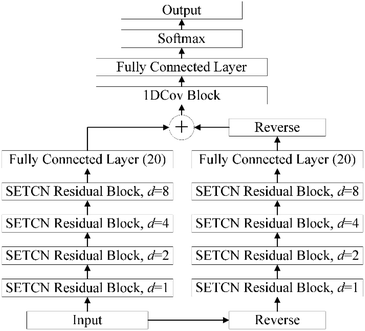
2.2.4. Architecture of SEBTCN. Secondary structure prediction is not only influenced by past information but also related to future information. However, SETCN using dilated causal convolution does not rely on future features for sequence prediction. Therefore, we propose SEBTCN to extract bidirectional key features in sequences.As shown in Fig. 4, the SEBTCN contains forward SETCN and backward SETCN. Let the protein sequence be X = {x1, x2, …, xL}24 and the reverse sequence be X← = {xL, xL−1, …, x1}, where L is the sequence length. SEBTCN can be calculated as:
| |
 | (9) |
| |
 | (10) |
| |
 | (11) |
where
Ŷ and
Ŷ1 represent the outputs of the forward and backward SETCN,

and

represent the forward and backward SETCN,
Output represents the output of SEBTCN, softmax represents the activation function,
F represents the operation of the fully connected layer, 1DCov represents operations such as convolution optimization of the 1DCov block,

represents the reverse vector of
Ŷ1, and ⊕ represents an element-wise addition operation.
 |
| | Fig. 4 The architecture of SEBTCN. | |
Therefore, our SEBTCN can not only extract key feature information but also extract bidirectional deep dependencies. Furthermore, SEBTCN can be applied to all classification problems.
2.3. Broad learning system (BLS)
BLS is a flat network based on random vector functional-link neural networks,32 which can effectively solve local optimal problems. As an efficient incremental learning system that does not require a deep network architecture, BLS has a simple structure, an efficient modeling process, and can be updated dynamically and incrementally. As shown in Fig. 5, the architecture of BLS mainly consists of three parts: feature mapping layer, enhancement node layer and output layer. The network can randomly map input features to feature nodes. Then, the mapped features are expanded to the generated enhancement nodes. Finally, feature nodes and enhancement nodes are connected to the output.
 |
| | Fig. 5 The architecture of the BLS. | |
Let the input feature matrix be X ∈ RN×D, and the secondary structure label be Y ∈ RN×C, where N is the number of samples, D is the sample dimension, and C is the number of categories. The mapping feature generated by the ith mapping feature node is:
| | |
Zi = ϕ(XWei + βei), i = 1, …, n
| (12) |
where
ϕ is the mapping function, and
W and
β are randomly generated weights and biases. To speed up the learning process during training, features are randomly mapped to enhancement nodes to improve nonlinear learning ability in feature extraction.
Let all feature nodes be Zn ![[triple bond, length half m-dash]](https://www.rsc.org/images/entities/char_e007.gif) [Z1, Z2, …, Zn], so the mth group of enhancement nodes can be calculated as:
[Z1, Z2, …, Zn], so the mth group of enhancement nodes can be calculated as:
| |
Hm ![[triple bond, length half m-dash]](https://www.rsc.org/images/entities/char_e007.gif) ξ(ZnWhm + βhm) ξ(ZnWhm + βhm)
| (13) |
where
ξ is the activation function of the enhancement node. BLS can be calculated as follows:
| |
 | (14) |
where
Wm = [
Zn|
Hm]
+Y is the output connection weight of BLS. Let
A = [
Zn|
Hm], the network computes
A+ by solving the ridge regression approximation:
| |
 | (15) |
2.4. The proposed DLBLS_SS
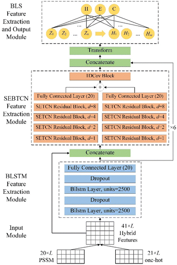
The detailed architecture of DLBLS_SS is shown in Fig. 6. To improve PSSP, the proposed model combines deep learning and BLS to predict 3-state and 8-state secondary structure. DLBLS_SS is mainly divided into four modules: input module, BLSTM feature extraction module, SEBTCN feature extraction module, BLS feature extraction and output module.
 |
| | Fig. 6 The detailed architecture of DLBLS_SS. | |
In the input module, we use the initial protein data to generate one-hot features and PSSM profiles. The input to the model is a 41 × L hybrid feature PSSM + one-hot, where L represents the residue length of the protein.
In the BLSTM feature extraction module, we use two BLSTM layers to extract global features in residue sequences. We also use a dropout layer after the BLSTM layer to avoid the risk of overfitting during training.
In SEBTCN feature extraction module, we fuse input features and global features extracted by BLSTM. We then use four SETCN residual blocks with channel attention to further bidirectionally capture key deep long-range dependencies between amino acid residues. Furthermore, a 1DCov block is used for fast optimization of features. The broad receptive field of SEBTCN can establish better long-range bidirectional interactions between sequence elements.
In the BLS feature extraction and output module, we first fuse the long-range features extracted by SEBTCN and BLSTM. Secondary structure prediction is mainly affected by local residues, so we use the sliding window technique to segment the fusion features into sequences of size 40 × 19 and further transform them so that the model can extract local interactions. We use 40 feature node groups with 40 nodes to transform the input data into the mapping feature space. Then, the mapping features are expanded in a broad sense to 10![[thin space (1/6-em)]](https://www.rsc.org/images/entities/char_2009.gif) 000 enhancement feature nodes for nonlinear learning. Finally, we obtain the output weights by computing the pseudo-inverse of the mapping and enhancement features to complete the classification of the secondary structure.
000 enhancement feature nodes for nonlinear learning. Finally, we obtain the output weights by computing the pseudo-inverse of the mapping and enhancement features to complete the classification of the secondary structure.
The proposed model can not only capture key long-range interactions in protein sequences but also utilize local optimal features for 3-state and 8-state PSSP. Furthermore, the powerful feature extraction capability of our model can better model complex sequence–structure relationships between input sequences and structural labels.
3 Experiments
3.1. Datasets
The PISCES33 server is widely used for PSSP, which can generate sequence subsets from the Protein Data Bank based on structural quality and mutual sequence identity. Therefore, we selected 14![[thin space (1/6-em)]](https://www.rsc.org/images/entities/char_2009.gif) 991 proteins using the PISCES server with parameters including: the percent identity cutoff was set to 25%, the resolution cutoff was set to 3 Å, and the R-factor cutoff was set to 0.25. We removed sequences that were duplicated with the test set. In addition, proteins with sequence lengths less than 40 or more than 800 were also deleted. The final constructed CullPDB33 dataset has 14
991 proteins using the PISCES server with parameters including: the percent identity cutoff was set to 25%, the resolution cutoff was set to 3 Å, and the R-factor cutoff was set to 0.25. We removed sequences that were duplicated with the test set. In addition, proteins with sequence lengths less than 40 or more than 800 were also deleted. The final constructed CullPDB33 dataset has 14![[thin space (1/6-em)]](https://www.rsc.org/images/entities/char_2009.gif) 562 proteins. For testing purpose, we randomly divided the dataset into training set (11
562 proteins. For testing purpose, we randomly divided the dataset into training set (11![[thin space (1/6-em)]](https://www.rsc.org/images/entities/char_2009.gif) 650), validation set (1456) and test set (1456). We randomly divided the dataset three times for classification three times. The final prediction accuracy is the mean of the three prediction accuracy.
650), validation set (1456) and test set (1456). We randomly divided the dataset three times for classification three times. The final prediction accuracy is the mean of the three prediction accuracy.
To evaluate the performance of the proposed model, we also use six public test sets CASP10,34 CASP11,35 CASP12,36 CASP13,37 CASP14 (ref. 38) and CB513,39 where all CASP datasets are available at https://predictioncenter.org/. The statistics of the six datasets are shown in Table 1.
Table 1 Number of proteins and residues in the six datasets
| Number |
CASP10 |
CASP11 |
CASP12 |
CASP13 |
CASP14 |
CB513 |
| Proteins |
99 |
81 |
19 |
22 |
23 |
513 |
| Residues |
24![[thin space (1/6-em)]](https://www.rsc.org/images/entities/char_2009.gif) 048 048 |
20![[thin space (1/6-em)]](https://www.rsc.org/images/entities/char_2009.gif) 084 084 |
4257 |
5948 |
4644 |
84![[thin space (1/6-em)]](https://www.rsc.org/images/entities/char_2009.gif) 119 119 |
3.2. Features
In this work, we use two feature representation methods one-hot encoding and PSSM as the input to the model. Amino acids include 20 standard amino acids (A, C, D, E, F, G, H, I, K, L, M, N, P, Q, R, S, T, V, W, Y and X) and 6 non-standard amino acids such as B, X, and Z. Because the number of non-standard amino acids is low, they can be classified as one type. Therefore, we can consider that amino acids have 21 types. The one-hot encoding method can represent each type of amino acid as a 21-dimensional vector, in which the corresponding component of the amino acid is 1, and the remaining components are 0. Since the vectors of the 21 amino acid types are mutually orthogonal, one-hot encoding can also be called orthogonal encoding.
PSSM is a scoring matrix generated by aligning the sequence itself with multiple sequences, which is widely used for feature representation. We use the PSI-BLAST40 procedure to generate PSSM profiles, where the threshold E is set to 0.001 and the number of iterations is set to 3. PSSM can express an amino acid sequence of length L as an L × 20 feature matrix by scoring 20 standard amino acid types.
3.3. Evaluation metrics
In this work, to evaluate the overall prediction accuracy of the proposed model, we use four commonly used metrics: Q3 accuracy, Q8 accuracy and SOV41 score for 3-state and 8-state PSSP. The secondary structure corresponding to the amino acid sequence was obtained by the DSSP5 program. Let the 3-state secondary structure S3 = {H, E, C}, and the 8-state secondary structure S8 = {G, I, H, B, E, S, T, C}. Q3 and Q8 overall accuracy is defined as:| |
 | (16) |
where N is the total number of residues and ns is the correct number of predicted type s. Let the total number of residues of the sequence be NSOV, the observed segment be S1, the predicted segment be S2, and the overlapping segment of S1 and S2 be S0. The SOV score can be calculated as follows:| |
 | (17) |
where maxov(S1, S2) and minov(S1, S2) represent the union length and overlap length of the segments S1 and S2, respectively. The σ(S1, S2) allowed to vary at the segment edges is calculated as:| |
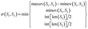 | (18) |
3.4. Performance analysis of the proposed model
In this section, to demonstrate the impact of the hyperparameters of the three modules in DLBLS_SS on the performance of 3-state and 8-state PSSP, we conduct extensive experiments using the CullPDB dataset.
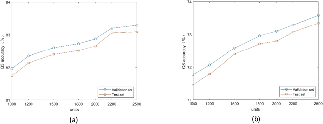
3.4.1. Influence of BLSTM module parameters. To explore the effect of the number of units in the BLSTM layer on the proposed method, we conduct comparative experiments on the validation and test sets. We use two BLSTM layers, which is the best number demonstrated experimentally. As shown in Fig. 7, the model achieves the highest Q3 and Q8 accuracy on two datasets when using 2500 units. Because the number of units directly affects the ability to analyze high-dimensional residue sequences, too many hidden units can also lead to network overfitting.
 |
| | Fig. 7 (a) Q3 accuracy of the proposed method under different number of units. (b) Q8 accuracy of the proposed method under different number of units. | |
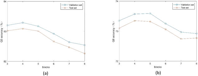
3.4.2. Influence of SEBTCN module parameters. Since the number of SETCN residual blocks determines the receptive field of the model, we use different numbers of residual blocks to classify the validation and test sets. As shown in Fig. 8, the model achieves the best 3-state PSSP performance when the number of residual blocks is 4, and the model achieves the best 8-state PSSP performance on the two datasets when the number of residual blocks is 4 and 5, respectively. The main reason is that the number of residual blocks affects the depth of the network. Also, too many residual blocks can trap the model in local optima.
 |
| | Fig. 8 (a) Q3 accuracy of the proposed method under different number of SETCN blocks. (b) Q8 accuracy of the proposed method under different number of SETCN blocks. | |
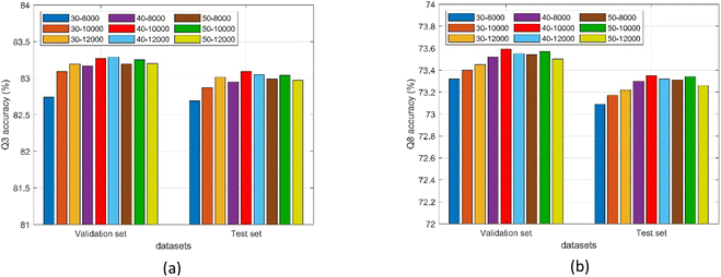
3.4.3. Influence of SEBTCN module parameters. The number of feature nodes and enhancement nodes in the BLS module determines the network width. Fig. 9 shows the 3-state and 8-state PSSP performance of the proposed method on validation and test sets under different numbers of nodes. The Q3 accuracy of the model on the two datasets reaches the maximum when the feature nodes are 40 and the enhancement nodes are 10![[thin space (1/6-em)]](https://www.rsc.org/images/entities/char_2009.gif) 000 and 12
000 and 12![[thin space (1/6-em)]](https://www.rsc.org/images/entities/char_2009.gif) 000 respectively. The model achieves the highest Q8 accuracy on two datasets when using 40 feature nodes and 10
000 respectively. The model achieves the highest Q8 accuracy on two datasets when using 40 feature nodes and 10![[thin space (1/6-em)]](https://www.rsc.org/images/entities/char_2009.gif) 000 enhancement nodes. Furthermore, the number of nodes not only determines the prediction performance but also affects the size of the model.
000 enhancement nodes. Furthermore, the number of nodes not only determines the prediction performance but also affects the size of the model.
 |
| | Fig. 9 (a) Q3 accuracy of the proposed method under different number of nodes. (b) Q8 accuracy of the proposed method under different number of nodes. | |
3.5. Ablation study
To demonstrate the effectiveness of the proposed models, we conduct comparative experiments with Q3 accuracy and Q8 accuracy as evaluation metrics. The comparison results of the six models on the seven datasets are shown in Table 2. Compared with SETCN, SEBTCN achieves an average improvement of 5.27% and 5.37% in Q3 accuracy and Q8 accuracy on seven datasets, which indicates that the proposed SEBTCN can sufficiently extract bidirectional key features in sequences. SETCN consistently outperforms LSTM in PSSP, while SEBTCN outperforms BLSTM in most cases, mainly because SEBTCN has a broad receptive field, but it also loses some important information. The integration of BLSTM and SEBTCN achieves higher 3-state and 8-state PSSP accuracy, which proves that SEBTCN can further extract long-range features. Furthermore, DLBLS_SS achieves better prediction performance compared to BLSTM + SEBTCN, which proves that the introduction of BLS can effectively extract local features to improve classification accuracy.
Table 2 3-state and 8-state PSSP results of six models on seven datasets. Bold indicates the best performance
| Models |
CullPDB |
CASP10 |
CASP11 |
CASP12 |
CASP13 |
CASP14 |
CB513 |
| Q3 |
Q8 |
Q3 |
Q8 |
Q3 |
Q8 |
Q3 |
Q8 |
Q3 |
Q8 |
Q3 |
Q8 |
Q3 |
Q8 |
| LSTM |
74.05 |
62.87 |
75.66 |
65.47 |
74.68 |
63.22 |
74.67 |
62.98 |
73.91 |
61.68 |
73.55 |
62.77 |
76.87 |
66.87 |
| SETCN |
75.62 |
64.79 |
77.79 |
66.95 |
75.73 |
64.89 |
76.14 |
64.85 |
74.96 |
63.01 |
74.69 |
63.85 |
80.11 |
68.12 |
| SEBTCN |
81.39 |
70.92 |
82.75 |
71.79 |
80.96 |
70.07 |
80.57 |
69.97 |
80.91 |
67.96 |
80.54 |
69.39 |
84.82 |
73.94 |
| BLSTM |
82.16 |
72.38 |
83.21 |
72.64 |
80.91 |
70.16 |
80.37 |
69.30 |
80.46 |
67.43 |
80.49 |
68.81 |
84.79 |
75.86 |
| BLSTM + SEBTCN |
82.97 |
73.22 |
83.73 |
73.54 |
81.60 |
71.52 |
81.14 |
70.39 |
81.27 |
68.41 |
81.18 |
69.97 |
85.74 |
77.06 |
| DLBLS_SS |
83.10 |
73.35 |
84.06 |
73.95 |
81.76 |
71.65 |
81.28 |
70.54 |
81.39 |
68.59 |
81.32 |
70.24 |
85.90 |
77.35 |
As shown in Table 3, we compare the prediction performance of the proposed model under different input features on seven datasets. When the input is the hybrid feature PSSM + one-hot, the prediction accuracy of DLBLS_SS reaches the maximum. Furthermore, it can be seen that PSSM features are significantly better than one-hot features, mainly because PSSM contains richer biological information.
Table 3 Q3 and Q8 accuracy of DLBLS_SS under different features on seven datasets. Bold indicates the best performance
| Features |
CullPDB |
CASP10 |
CASP11 |
CASP12 |
CASP13 |
CASP14 |
CB513 |
| Q3 |
Q8 |
Q3 |
Q8 |
Q3 |
Q8 |
Q3 |
Q8 |
Q3 |
Q8 |
Q3 |
Q8 |
Q3 |
Q8 |
| PSSM |
82.08 |
72.13 |
82.96 |
72.71 |
80.63 |
70.37 |
80.13 |
69.28 |
80.22 |
67.31 |
80.17 |
68.95 |
84.74 |
76.05 |
| One-hot |
72.74 |
62.79 |
73.59 |
63.18 |
72.27 |
61.97 |
72.79 |
62.01 |
71.92 |
59.57 |
72.41 |
61.21 |
75.02 |
65.97 |
| PSSM + one-hot |
83.10 |
73.35 |
84.06 |
73.95 |
81.76 |
71.65 |
81.28 |
70.54 |
81.39 |
68.59 |
81.32 |
70.24 |
85.90 |
77.35 |
3.6. Comparison with popular models
In this section, we compare the proposed method with five state-of-the-art methods DCRNN,42 CNN_BIGRU,43 DeepACLSTM,44 MUFOLD-SS45 and ShuffleNet_SS46 on seven test sets CullPDB, CASP10, CASP11, CASP12, CASP13, CASP14 and CB513. The DCRNN model utilizes a multi-scale convolutional neural network to extract local features and a bidirectional neural network composed of gated units to extract global features. The CNN_BIGRU model utilizes convolutional networks and bidirectional gating units to improve the accuracy of PSSP. The DeepACLSTM model predicts secondary structure using local and long-range dependencies extracted by asymmetric convolutional and bidirectional long short-term memory networks. The MUFOLD-SS predictor utilizes the deep inception-inside-inception method for prediction. ShuffleNet_SS introduces label distribution-aware margin loss in lightweight convolutional networks to improve rare class recognition. For the purpose of fair comparison, we use our dataset to train all models in the experiments, where the hybrid feature PSSM + one-hot is used as input.
To evaluate the prediction performance of the proposed model for 3-state and 8-state secondary structure, we employ Q3 accuracy, Q8 accuracy and SOV score as evaluation measures. The 3-state and 8-state PSSP comparison results of the proposed model and five existing popular models on seven benchmark datasets are shown in Tables 4 and 5. The comparison of Q3 accuracy and SOV score in Table 4 shows that DLBLS_SS exhibits better prediction performance in most cases compared to five popular methods. Table 5 shows that the 8-state PSSP performance of DLBLS_SS consistently outperforms the five state-of-the-art models on the seven test sets. This is mainly because the powerful analytical ability and broad receptive field of DLBLS_SS can effectively capture the key local and long-range dependencies in high-dimensional protein sequences, which can optimize the problem of insufficient feature extraction and enhance the ability of secondary structure recognition. Furthermore, we performed a paired t-test47 on the Q8 accuracy of each protein of these models on the CB513 dataset with a confidence level of 0.05. In the t-test, there are significant differences between DLBLS_SS and the other five state-of-the-art models. Among them, our model is the closest to the mean of ShuffleNet_SS.
Table 4 Performance comparison with state-of-the-art models on seven datasets in 3-state PSSP. Bold indicates the best performance
| Models |
CullPDB |
CASP10 |
CASP11 |
CASP12 |
CASP13 |
CASP14 |
CB513 |
| Q3 |
SOV |
Q3 |
SOV |
Q3 |
SOV |
Q3 |
SOV |
Q3 |
SOV |
Q3 |
SOV |
Q3 |
SOV |
| DCRNN |
82.12 |
78.51 |
82.57 |
75.71 |
80.57 |
75.53 |
80.41 |
74.75 |
80.49 |
77.09 |
80.27 |
71.46 |
84.65 |
79.63 |
| CNN_BIGRU |
82.32 |
78.68 |
82.42 |
76.20 |
81.05 |
76.58 |
80.38 |
75.62 |
80.66 |
76.94 |
80.46 |
71.92 |
84.83 |
79.90 |
| DeepACLSTM |
82.64 |
79.45 |
83.43 |
77.76 |
81.32 |
76.04 |
80.49 |
75.56 |
80.92 |
77.43 |
80.79 |
71.73 |
85.02 |
80.12 |
| MUFOLD-SS |
83.02 |
79.62 |
83.28 |
78.04 |
81.67 |
77.41 |
80.92 |
77.47 |
81.15 |
78.02 |
81.13 |
70.97 |
85.30 |
80.23 |
| ShuffleNet_SS |
83.06 |
78.79 |
83.85 |
76.27 |
81.70 |
76.37 |
80.87 |
76.39 |
81.41 |
77.46 |
81.24 |
71.32 |
85.61 |
79.98 |
| DLBLS_SS |
83.10 |
79.15 |
84.06 |
78.13 |
81.76 |
77.71 |
81.28 |
75.98 |
81.39 |
77.18 |
81.32 |
72.55 |
85.90 |
80.67 |
Table 5 Performance comparison with state-of-the-art models on seven datasets in 8-state PSSP. Bold indicates the best performance
| Models |
CullPDB |
CASP10 |
CASP11 |
CASP12 |
CASP13 |
CASP14 |
CB513 |
| Q8 |
SOV |
Q8 |
SOV |
Q8 |
SOV |
Q8 |
SOV |
Q8 |
SOV |
Q8 |
SOV |
Q8 |
SOV |
| DCRNN |
72.06 |
70.42 |
72.10 |
69.74 |
70.51 |
68.44 |
69.40 |
67.24 |
68.05 |
68.01 |
68.87 |
63.27 |
75.63 |
73.06 |
| CNN_BIGRU |
72.30 |
70.15 |
71.89 |
69.17 |
70.95 |
69.05 |
69.68 |
68.06 |
67.84 |
67.92 |
68.69 |
62.95 |
75.55 |
72.84 |
| DeepACLSTM |
72.87 |
71.34 |
73.08 |
71.42 |
71.24 |
69.93 |
69.82 |
68.18 |
68.46 |
69.31 |
69.55 |
63.46 |
76.02 |
73.46 |
| MUFOLD-SS |
73.32 |
71.59 |
72.99 |
71.51 |
71.59 |
69.84 |
70.22 |
69.32 |
68.23 |
68.89 |
69.24 |
62.69 |
76.64 |
74.04 |
| ShuffleNet_SS |
73.30 |
71.12 |
73.62 |
70.23 |
71.55 |
69.17 |
70.21 |
68.73 |
68.52 |
68.36 |
69.89 |
63.17 |
76.87 |
73.32 |
| DLBLS_SS |
73.35 |
71.96 |
73.95 |
72.07 |
71.65 |
70.04 |
70.54 |
69.34 |
68.59 |
69.33 |
70.24 |
63.58 |
77.35 |
75.08 |
4 Conclusions
In this paper, we combine deep learning and BLS to propose a novel model DLBLS_SS for 3-state and 8-state PSSP. In DLBLS_SS, the BLSTM module can extract global features in protein sequences, the SEBTCN module can bidirectionally capture key deep long-range dependencies in residue sequences, and the BLS module can further capture local interactions between residues while rapidly optimizing the extracted features. SEBTCN is our proposed sequence-to-sequence prediction network based on TCN and channel attention mechanism. We test the prediction performance of the proposed DLBLS_SS on the public test sets CASP10, CASP11, CASP12, CASP13, CASP14 and CB513 using the evaluation metrics Q3 accuracy, Q8 accuracy and SOV score. Experimental results show that the proposed DLBLS_SS exhibits state-of-the-art prediction performance compared to five popular models. The proposed model has powerful feature extraction ability, which can comprehensively utilize local and global optimal features for prediction to improve secondary structure recognition. In the future, we will continue to study techniques such as feature extraction and fusion in PSSP while exploring complex sequence–structure relationships.
Data availability
The dataset and code for this study are at https://github.com/yuanlu9707/DLBLS_SS.
Author contributions
LY, XH, YM and YL conceived the idea for this research. LY and XH implement the model. LY, XH and YM collected the data. LY and YM wrote the manuscript, YM and YL supervised the research and reviewed the manuscript. All authors contributed to the article and approved the submitted version.
Conflicts of interest
There are no conflicts to declare.
Acknowledgements
This work was supported by the National Natural Science Foundation of China [grant number 61375013] and the Natural Science Foundation of Shandong Province [grant number ZR2013FM020].
Notes and references
- Y. Yang, J. Gao, J. Wang, R. Heffernan, J. Hanson, K. Paliwal and Y. Zhou, Briefings Bioinf., 2018, 19, 482–494 CAS.
- P. Kumar, S. Bankapur and N. Patil, Appl. Soft Comput., 2020, 86, 105926 CrossRef.
- Y. Wang, H. Mao and Z. Yi, Knowl.-Based Syst., 2017, 118, 115–123 CrossRef.
- G. Wang, Y. Zhao and D. Wang, Neurocomputing, 2008, 72, 262–268 CrossRef.
- W. Kabsch and C. Sander, Biopolymers, 1983, 22, 2577–2637 CrossRef CAS PubMed.
- A. Yaseen and Y. Li, BMC Bioinf., 2014, 15, 1–8 CrossRef PubMed.
- Y. Ma, Y. Liu and J. Cheng, Sci. Rep., 2018, 8, 1–10 Search PubMed.
- S. Hua and Z. Sun, J. Mol. Biol., 2001, 308, 397–407 CrossRef CAS.
- B. Yang, Q. Wu, Z. Ying and H. Sui, Knowl.-Based Syst., 2011, 24, 304–313 CrossRef.
- S. Salzberg and S. Cost, J. Mol. Biol., 1992, 227, 371–374 CrossRef CAS PubMed.
- R. Bondugula, O. Duzlevski and D. Xu, Profiles and fuzzy k-nearest neighbour algorithm for protein secondary structure prediction, 2005 Search PubMed.
- N. Qian and T. J. Sejnowski, J. Mol. Biol., 1988, 202, 865–884 CrossRef CAS PubMed.
- E. Faraggi, T. Zhang, Y. Yang, L. Kurgan and Y. Zhou, J. Comput. Chem., 2012, 33, 259–267 CrossRef CAS PubMed.
- L. J. McGuffin, K. Bryson and D. T. Jones, Bioinformatics, 2000, 16, 404–405 CrossRef CAS PubMed.
- A. Drozdetskiy, C. Cole, J. Procter and G. J. Barton, Nucleic Acids Res., 2015, 43, W389–W394 CrossRef CAS PubMed.
- C. N. Magnan and P. Baldi, Bioinformatics, 2014, 30, 2592–2597 CrossRef CAS PubMed.
- S. Wang, J. Peng, J. Ma and J. J. Xu, Sci. Rep., 2016, 6, 1–11 CrossRef PubMed.
- J. Zhou and O. Troyanskaya, Deep supervised and convolutional generative stochastic network for protein secondary structure prediction, 2014 Search PubMed.
- R. Heffernan, Y. Yang, K. Paliwal and Y. Zhou, Bioinformatics, 2017, 33, 2842–2849 CrossRef CAS PubMed.
- J. Hanson, K. Paliwal, T. Litfin, Y. Yang and Y. Zhou, Bioinformatics, 2019, 35, 2403–2410 CrossRef CAS PubMed.
- M. S. Klausen, M. C. Jespersen, H. Nielsen, K. K. Jensen, V. I. Jurtz, C. K. Soenderby, M. O. A. Sommer, O. Winther, M. Nielsen and B. Petersen, Proteins: Struct., Funct., Bioinf., 2019, 87, 520–527 CrossRef CAS PubMed.
- M. R. Uddin, S. Mahbub, M. S. Rahman and M. S. Bayzid, Bioinformatics, 2020, 36, 4599–4608 CrossRef CAS PubMed.
- G. Xu, Q. Wang and J. Ma, Bioinformatics, 2020, 36, 5021–5026 CrossRef CAS PubMed.
- Z. Lyu, Z. Wang, F. Luo, J. Shuai and Y. Huang, Front. Bioeng. Biotechnol., 2021, 404 Search PubMed.
- J. Hu, L. Shen and G. Sun, Squeeze-and-excitation networks, 2018 Search PubMed.
- S. Bai, J. Z. Kolter and V. J. Koltun, An empirical evaluation of generic convolutional and recurrent networks for sequence modeling, 2018 Search PubMed.
- A. Graves and J. Schmidhuber, Neural Networks, 2005, 18, 602–610 CrossRef.
- C. P. Chen and Z. Liu, IEEE Trans. Neural Networks Learn. Syst., 2017, 29, 10–24 Search PubMed.
- D. T. Jones, J. Mol. Biol., 1999, 292, 195–202 CrossRef CAS PubMed.
- M. Schuster and K. K. Paliwal, IEEE Trans. Signal Process., 1997, 45, 2673–2681 CrossRef.
- S. Hochreiter and J. Schmidhuber, Neural Comput., 1997, 9, 1735–1780 CrossRef CAS PubMed.
- Y.-H. Pao and Y. Takefuji, IEEE Comput., 1992, 25, 76–79 Search PubMed.
- G. Wang and R. L. Dunbrack, Nucleic Acids Res., 2005, 33, W94–W98 CrossRef CAS PubMed.
- J. Moult, K. Fidelis, A. Kryshtafovych, T. Schwede and A. Tramontano, Proteins: Struct., Funct., Bioinf., 2014, 82, 1–6 CrossRef CAS PubMed.
- J. Moult, K. Fidelis, A. Kryshtafovych, T. Schwede and A. Tramontano, Proteins: Struct., Funct., Bioinf., 2016, 84, 4–14 CrossRef PubMed.
- J. Moult, K. Fidelis, A. Kryshtafovych, T. Schwede and A. J. P. S. Tramontano, Proteins: Struct., Funct., Bioinf., 2018, 86, 7–15 CrossRef CAS PubMed.
- A. Kryshtafovych, T. Schwede, M. Topf, K. Fidelis and J. Moult, Proteins: Struct., Funct., Bioinf., 2019, 87, 1011–1020 CrossRef CAS PubMed.
- A. Kryshtafovych, T. Schwede, M. Topf, K. Fidelis and J. Moult, Proteins: Struct., Funct., Bioinf., 2021, 89, 1607–1617 CrossRef CAS PubMed.
- J. A. Cuff and G. Barton, Proteins: Struct., Funct., Bioinf., 1999, 34, 508–519 CrossRef CAS.
- S. F. Altschul, T. L. Madden, A. A. Schäffer, J. Zhang, Z. Zhang, W. Miller and D. J. Lipman, Nucleic Acids Res., 1997, 25, 3389–3402 CrossRef CAS PubMed.
- A. Zemla, Č. Venclovas, K. Fidelis and B. Rost, Proteins: Struct., Funct., Bioinf., 1999, 34, 220–223 CrossRef CAS.
- Z. Li and Y. J. Yu, Protein secondary structure prediction using cascaded convolutional and recurrent neural networks, 2016 Search PubMed.
- I. Drori, I. Dwivedi, P. Shrestha, J. Wan, Y. Wang, Y. He, A. Mazza, H. Krogh-Freeman, D. Leggas and K. J. Sandridge, High quality prediction of protein q8 secondary structure by diverse neural network architectures, 2018 Search PubMed.
- Y. Guo, W. Li, B. Wang, H. Liu and D. Zhou, BMC Bioinf., 2019, 20, 1–12 CrossRef.
- C. Fang, Y. Shang and D. Xu, Proteins: Struct., Funct., Bioinf., 2018, 86, 592–598 CrossRef CAS PubMed.
- W. Yang, Z. Hu, L. Zhou and Y. J. Jin, Knowl.-Based Syst., 2022, 237, 107771 CrossRef.
- H. Hsu and P. A. Lachenbruch, Paired t test, 2014 Search PubMed.
|
| This journal is © The Royal Society of Chemistry 2022 |
Click here to see how this site uses Cookies. View our privacy policy here.  Open Access Article
 ,
Xiaopei Hu,
Yuming Ma* and
Yihui Liu*


 and
and  represent the forward and backward SETCN, Output represents the output of SEBTCN, softmax represents the activation function, F represents the operation of the fully connected layer, 1DCov represents operations such as convolution optimization of the 1DCov block,
  represents the reverse vector of Ŷ1, and ⊕ represents an element-wise addition operation.
![[triple bond, length half m-dash]](https://www.rsc.org/images/entities/char_e007.gif) [Z1, Z2, …, Zn], so the mth group of enhancement nodes can be calculated as:
[Z1, Z2, …, Zn], so the mth group of enhancement nodes can be calculated as:![[triple bond, length half m-dash]](https://www.rsc.org/images/entities/char_e007.gif) ξ(ZnWhm + βhm)
ξ(ZnWhm + βhm)


![[thin space (1/6-em)]](https://www.rsc.org/images/entities/char_2009.gif) 000 enhancement feature nodes for nonlinear learning. Finally, we obtain the output weights by computing the pseudo-inverse of the mapping and enhancement features to complete the classification of the secondary structure.
000 enhancement feature nodes for nonlinear learning. Finally, we obtain the output weights by computing the pseudo-inverse of the mapping and enhancement features to complete the classification of the secondary structure.![[thin space (1/6-em)]](https://www.rsc.org/images/entities/char_2009.gif) 991 proteins using the PISCES server with parameters including: the percent identity cutoff was set to 25%, the resolution cutoff was set to 3 Å, and the R-factor cutoff was set to 0.25. We removed sequences that were duplicated with the test set. In addition, proteins with sequence lengths less than 40 or more than 800 were also deleted. The final constructed CullPDB33 dataset has 14
991 proteins using the PISCES server with parameters including: the percent identity cutoff was set to 25%, the resolution cutoff was set to 3 Å, and the R-factor cutoff was set to 0.25. We removed sequences that were duplicated with the test set. In addition, proteins with sequence lengths less than 40 or more than 800 were also deleted. The final constructed CullPDB33 dataset has 14![[thin space (1/6-em)]](https://www.rsc.org/images/entities/char_2009.gif) 562 proteins. For testing purpose, we randomly divided the dataset into training set (11
562 proteins. For testing purpose, we randomly divided the dataset into training set (11![[thin space (1/6-em)]](https://www.rsc.org/images/entities/char_2009.gif) 650), validation set (1456) and test set (1456). We randomly divided the dataset three times for classification three times. The final prediction accuracy is the mean of the three prediction accuracy.
650), validation set (1456) and test set (1456). We randomly divided the dataset three times for classification three times. The final prediction accuracy is the mean of the three prediction accuracy.
![[thin space (1/6-em)]](https://www.rsc.org/images/entities/char_2009.gif) 048
048![[thin space (1/6-em)]](https://www.rsc.org/images/entities/char_2009.gif) 084
084![[thin space (1/6-em)]](https://www.rsc.org/images/entities/char_2009.gif) 119
119


![[thin space (1/6-em)]](https://www.rsc.org/images/entities/char_2009.gif) 000 and 12
000 and 12![[thin space (1/6-em)]](https://www.rsc.org/images/entities/char_2009.gif) 000 respectively. The model achieves the highest Q8 accuracy on two datasets when using 40 feature nodes and 10
000 respectively. The model achieves the highest Q8 accuracy on two datasets when using 40 feature nodes and 10![[thin space (1/6-em)]](https://www.rsc.org/images/entities/char_2009.gif) 000 enhancement nodes. Furthermore, the number of nodes not only determines the prediction performance but also affects the size of the model.
000 enhancement nodes. Furthermore, the number of nodes not only determines the prediction performance but also affects the size of the model.

