
 Open Access Article
 This Open Access Article is licensed under a Creative Commons Attribution-Non Commercial 3.0 Unported Licence
Uncertainty quantification for predictions of atomistic neural networks†
Luis Itza
Vazquez-Salazar
 a,
Eric D.
Boittier
b and
Markus
Meuwly
*cd
a,
Eric D.
Boittier
b and
Markus
Meuwly
*cd
aDepartment of Chemistry, University of Basel, Basel, Switzerland. E-mail: luisitza.vazquezsalazar@unibas.ch
bDepartment of Chemistry, University of Basel, Basel, Switzerland
cDepartment of Chemistry, University of Basel, Basel, Switzerland. E-mail: m.meuwly@unibas.ch
dDepartment of Chemistry, Brown University, USA
First published on 17th October 2022
Abstract
The value of uncertainty quantification on predictions for trained neural networks (NNs) on quantum chemical reference data is quantitatively explored. For this, the architecture of the PhysNet NN was suitably modified and the resulting model (PhysNet-DER) was evaluated with different metrics to quantify its calibration, the quality of its predictions, and whether prediction error and the predicted uncertainty can be correlated. Training on the QM9 database and evaluating data in the test set within and outside the distribution indicate that error and uncertainty are not linearly related. However, the observed variance provides insight into the quality of the data used for training. Additionally, the influence of the chemical space covered by the training data set was studied by using a biased database. The results clarify that noise and redundancy complicate property prediction for molecules even in cases for which changes – such as double bond migration in two otherwise identical molecules – are small. The model was also applied to a real database of tautomerization reactions. Analysis of the distance between members in feature space in combination with other parameters shows that redundant information in the training dataset can lead to large variances and small errors whereas the presence of similar but unspecific information returns large errors but small variances. This was, e.g., observed for nitro-containing aliphatic chains for which predictions were difficult although the training set contained several examples for nitro groups bound to aromatic molecules. The finding underlines the importance of the composition of the training data and provides chemical insight into how this affects the prediction capabilities of a ML model. Finally, the presented method can be used for information-based improvement of chemical databases for target applications through active learning optimization.
1 Introduction
Undoubtedly machine learning (ML) models are becoming part of the standard computational/theoretical chemistry toolbox. This is because it is possible to develop highly accurate trained models in an efficient manner. In chemistry, such ML models are used in various branches ranging from the study of reactive processes,1,2 sampling equilibrium states,3 the generation of accurate force fields,4–8 to the generation and exploration of chemical space.9–11 Nowadays, an extensive range of robust and complex models can be found.12–16 The quality of these models is only limited by the quality and quantity of the data used for training.7,17 For the most part, however, the focus was on obtaining more extensive and complex databases as an extrapolation from applications in computer science. Therefore, it is believed that more significant amounts of data will beat the best algorithms.18On the other hand, it has been found that even the best model can be tricked by poor data quality.19–22 For example, in malware detection it was found that ML-based models can fail if the training data does not contain the event the model had been designed for.19,21 The notion of underperforming models trained on low-quality data (“garbage in-garbage out”) can be traced back to Charles Babbage.23 The ML community is starting to notice the importance of data quality used for training and the relevance to balance amount of data (“big data”) versus quality of data. From other fields in Science, it is known that using biased and low-quality data in ML can result in catastrophic outcomes24 such as discrimination towards minorities,25 reduction in patient survival, and the loss of billions of dollars.26 As a result of these findings, the concept of “smart data” emerged27–29 which describes data sets that contain validated, well-defined and meaningful information that can be processed.28 However, specifically for chemical applications, an important additional consideration concerns the type of data that is required for predicting a particular target property.
Considering that data generation for training quantum ML models implies the use of considerable amounts of computational power30–32 which increases the carbon footprint and makes the use of ML difficult for researchers without sufficient resources, it is essential to optimize the full workflow from conception to a trained model. With this in mind, the concept of smart data is of paramount importance for conceiving future ML models in chemistry. This necessity has been considered in previous reviews about ML in chemistry;7,17 however, it is still poorly understood how the choice of training data influences the prediction quality of a trained machine-learned model. One such effort quantitatively assessed the impact of different commonly used quantum chemical databases on predicting specific chemical properties.33 The results showed that the predictions from the ML model are heavily affected by data redundancy and noise implicit in the generation of the training dataset.
Identifying missing/redundant information in chemical databases is a challenging but necessary step to ensure the best performance of ML models. In transfer learning from a lower level of quantum chemical treatment (e.g. Møller–Plesset second order theory – MP2) to the higher coupled cluster with singles, doubles and perturbative triples (CCSD(T)) it has been found for the H-transfer barrier height in malonaldehyde (MA) that it is the selection of geometries included in TL rather than the number of additional points that leads to a quantitatively correct model.34 This has been further confirmed by computing tunneling splittings for MA from quantum instanton calculations.35 It is also likely that depending on the chemical target quantity of interest the best database differs from the content of a more generic chemical database. Under such circumstances, uncertainty quantification (UQ) on the prediction provides valuable information on how prediction quality depends on the underlying database used for training the statistical model.
For chemical applications, ensemble methods which involve the training and evaluation of several independently trained statistical models to obtain the quantities of interest (average and variance for an observation) have been used.36,37 Despite their widespread use their disadvantage is the high computational cost they incur. An alternative to this are methods based on Gaussian process regression.38,39 However, these are limited by the size of the database that can be used. As ML models become more prevalent in different fields, new and efficient techniques for UQ have emerged which are potentially useful in chemical applications as well. These include Bayesian NNs40 and single deterministic networks41 with good prospects to be used in chemistry. One challenge for Bayesian NNs is that they need to be able to predict probability distributions over network parameters. This can become computationally intractable for NNs with a large number of parameters and data.40 On the other hand, single deterministic networks are of particular interest because they are computationally cheaper given that these models need to train and evaluate only one model allowing to predict the variance for forecasting using a single deterministic model.
Some methods for UQ based on single deterministic networks have been proposed, among them regression prior networks,42 mean variance estimation,43 or Deep Evidential Regression (DER).44 This last method has been recently applied in molecular discovery and inference for virtual screening.45 In a recent benchmark study43 four different UQ approaches were tested on a range of datasets. However, none of the methods tested performed best on all tasks. Part of this finding may be related to the notion that 2D networks were applied to the 3D problem of molecular structure which implies that such methods do not describe the system adequately and are not suitable to for uncertainty prediction.43 Finally, it was concluded that UQ is a challenging task which can be highly specific for the problem at hand. However, high dimensional NNs together with random forest or mean variance estimation (which is a type of single deterministic networks) were among the best-performing approaches.
The aim of the present study is twofold. First a model for uncertainty prediction and quantification rooted in deep evidential regression is implemented as a final layer in a message passing NN based on the PhysNet architecture. This model is referred to as PhysNet-DER. Starting from the QM9 dataset a variety of metrics for hyperparameter optimization are tested quantitatively. Secondly, the trained model is used to address two concrete chemical questions at a molecular level to highlight the value of UQ in practical applications. They include characterization of a biased database and the prediction of tautomerization energies. Both applications pose different challenges to the trained model and associated uncertainty quantification in that details of chemical bonding encoded in the data set used for training directly impacts the quality of the predictions. Finally, the results are discussed in a broader context.
2 Methods
As a regression model, PhysNet46 was selected for the present purpose. PhysNet was implemented within the PyTorch framework47 to make it compatible with modern GPU architectures and in line with community developments. The original architecture of PhysNet was modified to output the energy and three extra parameters required for the representation of the uncertainty (Fig. 1). Following earlier work,44 it is assumed that the targets to predict (here energies E_i for samples i) are drawn from an independent and identically distributed (i. i. d) Gaussian distribution with unknown mean (μ) and variance (σ2) for which probabilistic estimates are desired:
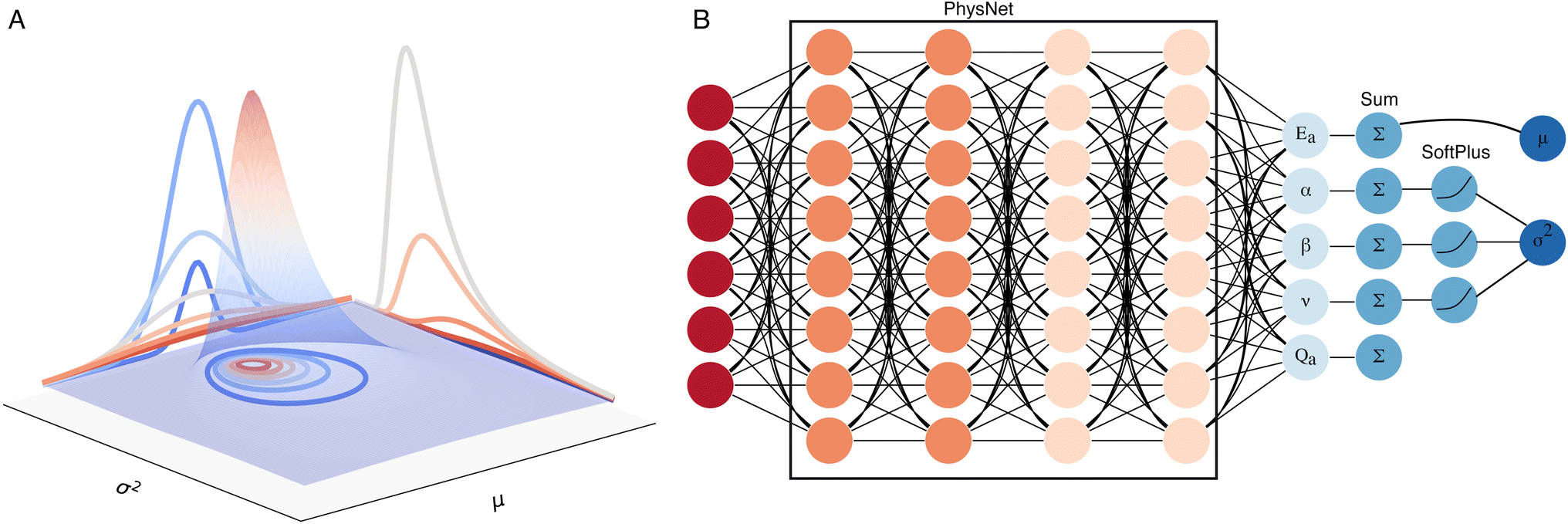 | ||
| Fig. 1 Modified PhysNet for uncertainty quantification. (A) Schematic 3D representation of the negative inverse gamma distribution as a function of the mean (μ) and the variance (σ2) (See eqn (1)). (B) The modified architecture of PhysNet for the addition of the ‘evidential’ layer. The input layer receives atomic positions, atomic numbers, charges, and energies. In the next step, those values are passed to the regular architecture of PhysNet. The final layer is modified to output five values (Ea, Qa, α, β, and ν) per each atom in a molecule. In the next step, the values of the outputs are summed by each molecule. Then, the three extra parameters are passed to a SoftPlus activation function (See eqn (3)). The final output of the model are the values that characterize the normal inverse gamma distribution. The mean value for the prediction (eqn (4)) corresponds to the energy of the predicted molecule, and the parameters to determine the variance of the predicted energy which can be obtained using eqn (5) and (6). | ||
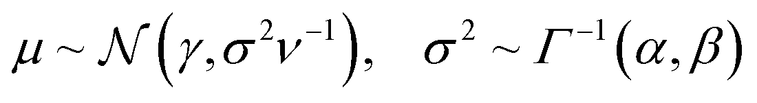
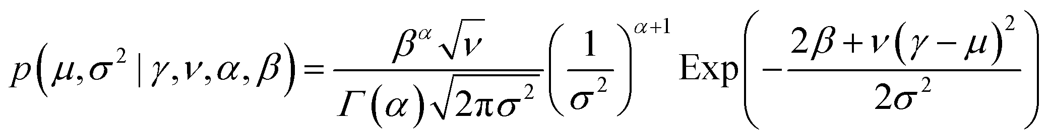
For modeling the unknown energy distribution, a prior distribution is placed on the unknown mean (μ) and variance (σ2). Following the assumption that the values are drawn from a Gaussian distribution, the mean can be represented by a Gaussian distribution and the variance as an inverse-gamma distribution
 , ν > 0, α > 1 and β > 0.
The desired posterior distribution has the form:
| q(μ, σ2) = p(μ,σ2|E1,…,EN). |
 | (1) |
The four parameters that represent the normal-inverse gamma distribution are the output of the final layer of the trained PhysNet model (Fig. 1) and the total predicted energy for a molecule composed of N atoms is obtained by summation of the atomic energy contributions Ei:
 | (2) |
In a similar fashion, the values for the three parameters (ν, α, and β) that describe the distribution of the variance for a molecule composed of N atoms are obtained by summation of the atomic contributions and are then passed to a softplus activation function to fulfill the conditions given for the distribution ( and ν, α, β > 0)
 | (3) |
Finally, the expected mean (eqn (4)), and the aleatory (eqn (5)) and epistemic (eqn (6)) uncertainty of predictions can be calculated as:
 | (4) |
 | (5) |
 | (6) |
Including the new parameters in the output of the neural network changes the loss function of the model. The new loss function consists of a dual-objective loss  with two terms: the first term maximizes model fitting and the second penalizes incorrect predictions according to
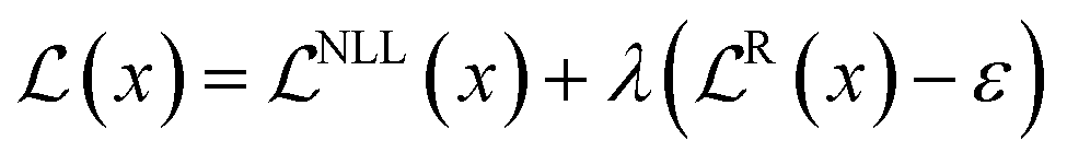 | (7) |
In eqn (7), the first term corresponds to the negative log-likelihood (NLL) of the model evidence that can be represented as a Student-t distribution (eqn (8))
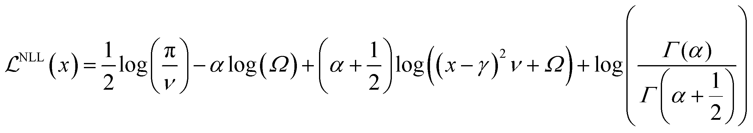 | (8) |
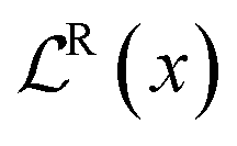 , corresponds to a regularizer that minimizes the evidence for incorrect predictions (eqn (9)).
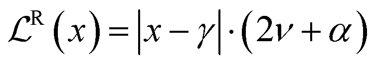 | (9) |
The hyperparameter λ controls the influence of uncertainty inflation on the model fit and can be calibrated to obtain more confident predictions. For λ = 0, the model is overconfident. i.e. results are less likely to be correct. Alternatively, for λ > 0, the variance is inflated, resulting in underconfident predictions.
The neural network architecture was that of standard PhysNet, with 5 modules consisting of 2 residual atomic modules and 3 residual interaction modules. Finally, the result is pooled into one residual output module. The number of radial basis functions was kept at 64, and the dimensionality of the feature space was 128. Electrostatic and dispersion corrections were not used for the training to keep the model as simple as possible. All other parameters were identical to the standard version of PhysNet,46 unless mentioned otherwise.
For training, a batch size of 32 and a learning rate of 0.001 were used. An exponential learning rate scheduler with a decay factor of 0.1 every 1000 steps and the ADAM optimizer48 with a weight decay of 0.1 were employed. An exponential moving average for all the parameters was used to prevent overfitting. A validation step was performed every five epochs.
2.1 Hyperparameter optimization
The hyperparameter λ in eqn (7) was optimized by training a range of models with different values of λ, using a portion of the QM9 dataset consisting of 31![[thin space (1/6-em)]](https://www.rsc.org/images/entities/char_2009.gif) 250 structures: 25000 structures for training, 3125 for validation and the remaining 3125 for testing. The splitting of the selected molecules of QM9 was performed randomly. The top panel of Fig. S7† shows that the energy distributions from the training and test sets overlap closely which demonstrates that the dataset used for training is representative of the overall distribution of energies. Models were trained for 1000 epochs and the values for λ were 0.01, 0.1, 0.2, 0.4, 0.5, 0.75, 1.0, 1.5, and 2.0. The calibration of the NN models is required to assure that the computed uncertainties can be related with the obtained errors on the prediction. It should be mentioned that although this procedure is computationally expensive, it only needs to be done once.
250 structures: 25000 structures for training, 3125 for validation and the remaining 3125 for testing. The splitting of the selected molecules of QM9 was performed randomly. The top panel of Fig. S7† shows that the energy distributions from the training and test sets overlap closely which demonstrates that the dataset used for training is representative of the overall distribution of energies. Models were trained for 1000 epochs and the values for λ were 0.01, 0.1, 0.2, 0.4, 0.5, 0.75, 1.0, 1.5, and 2.0. The calibration of the NN models is required to assure that the computed uncertainties can be related with the obtained errors on the prediction. It should be mentioned that although this procedure is computationally expensive, it only needs to be done once.
2.2 Metrics for model assessment and classification
In order to compare the performance/quality of the trained models, suitable metrics are required. These metrics are used to select the best value for the hyperparameter λ. Different metrics that have been reported in the literature49–51 were evaluated.The first metric considered is the Root Mean Variance (RMV) defined as:
 | (10) |
The next metric was the empirical Root Mean Squared Error (RMSE):
 | (11) |
 | (12) |
 | (13) |
In eqn (13), μσ is the mean predicted standard deviation and σt is the predicted standard deviation for M samples.
The last metric used for the characterization of the predicted variance of the tested models is the ‘sharpness'
 | (14) |
In eqn (14), the value Var(Fn) corresponds to the variance of the random variable with cumulative distribution function F at point n.50 The purpose of this metric is to measure how close the predicted values of the uncertainty are to a single value.52
In addition to the above metrics, calibration diagrams were constructed with the help of the uncertainty toolbox suite.53 Calibration diagrams report the frequency of correctly predicted values in each interval relative to the predicted fraction of points in that interval.50,54 Another interpretation of the calibration diagram is to quantify the “honesty” of a model by displaying the true probability in which a random variable is observed below a given quantile; if a model is calibrated this probability should be equal to the expected probability in that quantile.53
The results obtained for the test dataset were then classified into four different categories following the procedure described in Kahle and Zipoli.55 For the present purpose, ε* = MSE (mean squared error) and σ* = MV (mean variance), and the following classes were distinguished:
• True Positive (TP): εi > ε* and σi > σ*. The NN identifies a molecule with a large error through a large variance. In this case, it is possible to add training samples with relevant chemical information to improve the prediction of the identified TP. Alternatively, additional samples from perturbed structures for a particular molecule could be added to the increase chemical diversity.
• False Positive (FP): εi < ε* and σi > σ* in which case the NN identifies a molecule as a high-error point but the prediction is correct. In this case, the model is underconfident about its prediction.
• True Negative (TN): εi < ε* and σi < σ*. Here the model recognizes that a correct prediction is made with a small value for variance. For such molecules the model has sufficient information to predict them adequately by assigning a small variance. Therefore, the model does not require extra chemical information for an adequate prediction.
• False Negative (FN): εi > ε* and σi < σ*. The model is confident about its prediction for this molecule but it actually performs poorly on it. One possible explanation for this behaviour is that molecules in this category are rare56 in the training set. The model recognizes them with a small variance but because there is not sufficient information the target property (here energy) cannot be predicted correctly.
In the above classifications, i refers to a particular molecule considered for the evaluation. The classification relies on the important assumption that the MSE and the MV are comparable in magnitude which implies that the variance predicted by the model is a meaningful approximation to the error in the prediction. A second desired requirement is to assure the validity of the classification procedure and that the obtained variance is meaningful is that MSE > MV. This requirement is a consequence of the bias-variance decomposition of the squared error57
 | (15) |
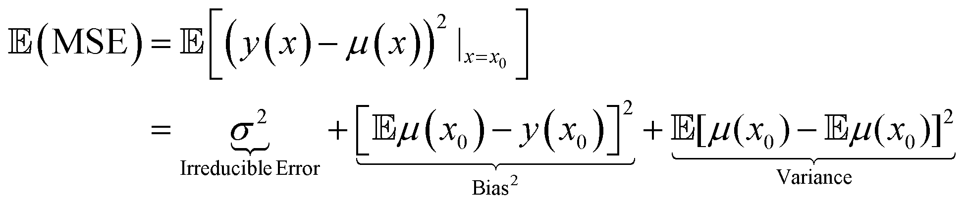
Eqn (15) states that the expected value  of the MSE consists of three terms: the irreducible error, the bias, and the variance. Therefore, the MSE will always be smaller than the variance except for the case that μ(x) = y for which those quantities are equal.58
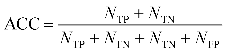
As a measure of the overall performance of the model, the accuracy is determined as:59
 | (16) |
In eqn (16), NTP, NTN, NFP, and NFN refers to the number of true positive, true negative, false positive, and false negative samples, respectively. Additionally, it is possible to compute the true positive rate (RTP) or sensitivity as:
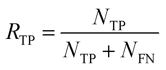 | (17) |
As a complement to eqn (17), the true positive predictive value (PTP) or precision is
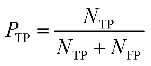 | (18) |
2.3 Model performance for tautomerization
As a final test, the performance of the evidential model was evaluated using a subset of the Tautobase,60 a public database containing 1680 pairs. Previously, those molecules were calculated at the level of theory of the QM9 database.33,61 For the purpose of the present work, only molecules that contain less than nine heavy atoms were included. Three neural networks with λ values of 0.2, 0.4, and 0.75 were trained with the QM9 database. The QM9 database was filtered to remove molecules containing fluorine and those that did not pass the geometry consistency check. The size of final database size was 110426 molecules. That number was split on 80% for training, 10% for validation and 10% for testing. The three models were trained for 500 epochs with the same parameters as for the hyperparameter optimization.
3 Results
In this section the calibration of the network is analyzed and its performance for different choices of the hyperparameter is assessed. Then, an artificial bias experiment is carried out and finally, the model is applied to the tautomerization data set. Before detailing these results, a typical learning curve for the model is shown in Fig. S1.† As expected, the root mean squared error obtained for the test set decreases with increasing number of samples. For the mean variance, see Fig. S2,† it is found that its magnitude reduces up to a certain size of the training set after which it increases again. This observation is further discussed in “Discussion and conclusions”.3.1 Calibration of the neural network
The selection of the best value for the hyperparameter λ can be related to the calibration of the neural network model. Ideally, a calibrated regression model should fulfill the condition49 thatwhere
 is the expected value for the squared difference of the predicted mean evaluated at x minus the observed value y. In other words: the squared error for a prediction can be directly related to the variance predicted by the model.49
Fig. 2 compares the root mean squared error with the root mean variance for a number of bins (N = 100) and shows that the correlation between RMSE and RMV can change between different intervals. Analyses were also carried out for different numbers N of bins and the effect on RMV was found to be negligible, see Fig. S3.† Additionally, the slope of the data can be used as an indicator as to whether the model over- or underestimates the error in the prediction. A slope closer to 1 indicates that the model is well-calibrated. Consequently, the predicted variance can be used as an indicator of the error with respect to the value to be predicted. The results in Fig. 2 also show that smaller values of λ = (0.01, 0.2, 0.4) result in increased slopes of the RMSE vs. RMV curve, i.e. leads to less well-calibrated models, resulting in a model that is overconfident in its predictions. Results that are more consistent with a slope of 1 are obtained for λ = 1. However, for all trained models it is apparent that RMSE and RMV are not related by a “simple” linear relationship as is sometimes assumed in statistical modeling.
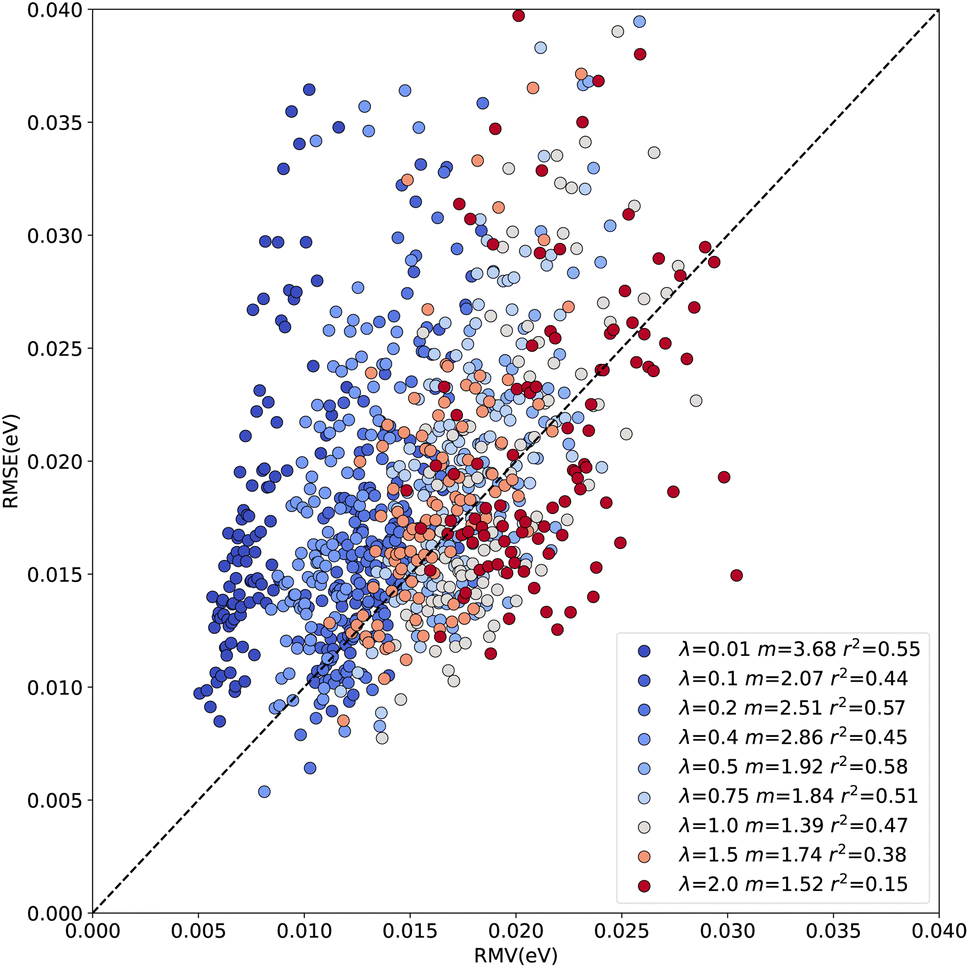 | ||
| Fig. 2 Empirical root mean squared error compared with the root mean variance of the evidential model trained on 25000 structures from the QM9 database. The values were divided in 100 bins ranked with respect to the predicted variance, 25 bins with 32 samples and 75 with 31 samples were considered. The value of λ together with the slope (m) from a linear regression analysis and the Pearson correlation coefficient (r2) are given in the legend. | ||
In previous studies,50 the dispersion of the predicted standard deviation was considered as a measure of the quality of a regression model. Hence a wider distribution of the predicted standard deviation by the model is desired. To remove the influence of pronounced outliers, Fig. 3A shows the distributions up to 99% of the predicted variance. It is clear that the center of the distribution, and its width, depend on λ. Larger values of the hyperparameter lead to wider distributions. However, the displacement of the center of mass of the distribution indicates that the standard deviation will be consistently overestimated. Also, p(σ) is not Gaussian but rather resembles the inverse gamma distribution that was used as prior for the variance.
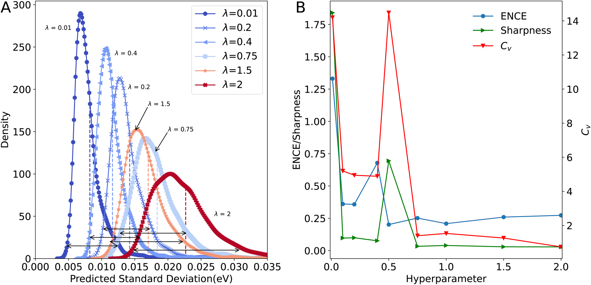 | ||
Fig. 3 Metrics for the distribution of predicted variance. (A) Kernel density estimate of standard deviation (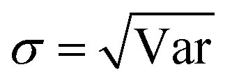 ) for different values of hyperparameter λ. Values up to the 99% percentile of the variance were considered. The internal arrows show the ‘width’ of the distributions. Dotted lines inside the distribution report their sharpness. Not all distributions are shown for clarity. (B) Evolution of the Expected Normalized Calibration Error (ENCE), sharpness, and the Coefficient of Variation (Cv) depending on λ. ) for different values of hyperparameter λ. Values up to the 99% percentile of the variance were considered. The internal arrows show the ‘width’ of the distributions. Dotted lines inside the distribution report their sharpness. Not all distributions are shown for clarity. (B) Evolution of the Expected Normalized Calibration Error (ENCE), sharpness, and the Coefficient of Variation (Cv) depending on λ. | ||
Predicted standard deviations from machine learned models must follow some characteristics that help to assess the quality of model predictions.50 Among those characteristics, it is expected that the distribution of the predicted variance is narrow, i.e. will be ‘sharp’. This has two objectives, the first is that the model returns uncertainties that are as tight as possible to a specific value.52 With this property the model gains confidence on its prediction. The second goal of a ‘sharp’ model is that it is able to capture the ‘trueness',62i.e. the distance between the true value and the mean of the predictions, on the forecast. Another desired characteristic is that p(σ) is disperse and does not return a constant value for the uncertainty which would make the model likely to fail for predictions on molecules outside the training data and compromise its generalizability.
The previously described characteristics of the distribution of uncertainties are related to the value of the hyperparameter λ in the loss function (eqn (7)) because, as can be seen in Fig. S6,† the MSE by percentile is independent on the choice of λ. Therefore, the model should be calibrated by selecting a value of the hyperparameter that fulfills the desired characteristics for the distribution of uncertainties.
Fig. 3A shows that the spread of the distribution of standard deviations increases with increasing λ. However, the second desired feature for those distribution – sharpness – decreases with increasing λ to become almost constant for λ ≥ 0.75. In consequence of this contradictory behaviour, it is necessary to find a value of λ that yields an accurate estimation of the uncertainty but it does not return a distribution of uncertainties but rather a constant value for each case. It is important to notice that both characteristics, sharpness and width of the distribution, are equally important and one of them should not be sacrificed in favour of the other.50 In other words: a calibrated model is characterized by uncertainty distributions with a certain sharpness and a certain width.
A deeper understanding of the difference between the error of a predicted value and the predicted variance can be obtained through the ENCE (eqn (12)) as described in the Methods section. This metric is similar to the expected calibration error used in classification.50 The ENCE quantifies the probability that the model incorrectly predicts the uncertainty of the prediction made. Fig. 3B reports the values of ENCE (blue line) and shows that, typically, smaller values for ENCE are expected for increasing hyperparameter λ. For λ = 0.4, the value of ENCE increases as opposite of the expected trend because the predicted value of the RMSE is larger than the value for RMV for most of the considered bins. However, it is clear that for λ ≥ 0.5, the ENCE is almost constant – which indicates that, on average, the model has a low probability to make incorrect predictions.
As a complement to the ENCE metric, the coefficient of variation (Cv) was also computed (red trace in Fig. 3B). This metric is considered to be less informative because the dispersion of the prediction depends on the validation/test data distribution.50,63 However, it is useful to characterize the spread of standard deviations because it is desired that the predicted uncertainties are spread and therefore cover systems outside the training data which help to generalize the model and make it transferable to molecules outside the training set. Comparing the results from Fig. 3A and the values for Cv in Fig. 3B, it is found that the largest dispersion is obtained for small values of λ. This indicates that the standard deviations for all predictions are concentrated in a small range of values for values in the 95th percentile of the distribution. For λ ≥ 0.75 both ENCE and Cv values do not show pronounced variation. It should be noted that the distributions in Fig. 3A are restricted to the 99% quantile of the data; on the other hand, the values for Cv covered the whole range of data. If the complete range of data is analyzed, it is possible to arrive at wrong conclusions. Fig. 3B shows that for λ = 0.5, the Cv value is large which suggests a flat distribution (Fig. S4†), however it should be noticed that this behaviour arises primarily due to pronounced outliers that impact the averages used for the calculation. However, 95% of the distribution is concentrated around a small range of variances as shown in Fig. 3A. Nevertheless, if only 95% of the data is studied, it is found that λ ≥ 0.5 yields increased CV (see Fig. S5†).
As shown in Fig. 3A, the center of mass of P(σ) displaces to larger σ with increasing λ. A more detailed analysis of the difference between MSE and MV for different percentiles of the variance was performed (Fig. S6†). Following the bias-variance decomposition of the squared error (eqn (15)), the bias of the model can be quantified as a function of the different values of λ. Fig. S6† shows that the MSE is constant regardless of the value of the hyperparameter λ or the percentile of the variance. On the other hand, the variance increases as a function of λ but it is constant regarding the value of the percentile with the exception of λ = 1. Thus, the MV is larger than the MSE which is counter-intuitive in view of the bias-variance decomposition of the squared error. Finally, it is clear that the difference between MSE and MV decreases as the value of λ increases. This indicates that the assumed posterior distribution does not correctly describe the data and, as a consequence, it cannot adequately capture the variance of a prediction. In other words, a better “guess” of the posterior will improve the predicted variance.
A common method to judge whether a model is well-calibrated is by considering the calibration curves described in the Methods section. The results in Fig. 4 show that, as λ increases, the model is closer to the diagonal which indicates perfect calibration. The best calibrated models are obtained for small values of λ (λ = 0.1 and λ = 0.2). Calibration curves help to evaluate the ‘honesty’ of the model predictions. Previously,45 calibration curves were employed to select a suitable value for λ using the SchNet architecture64 for QM9. These results largely agree with what is found here with λ = 0.1 and λ = 0.2 as the best values. Although calibration curves are extensively used in the literature to assess the quality of uncertainty predictions by ML models, they also have weaknesses that complicate their use. For example, it was reported49 that perfect calibration is possible for a model even if the output values are independent of the observed error. Furthermore, it was noticed49 that calibration curves work adequately when the uncertainty prediction is degenerate (i.e. all the output distributions have the same variance) which is not the desired behavior. In addition to this, it was found that the shape of these curves can be misleading because there are percentiles for which the model under- or overestimates the uncertainty. Then the calibration curves need to be complemented with additional metrics for putting their interpretation in perspective. Here, the analysis of calibration curves was complemented by using the miscalibration area (the area between the calibration curve and the diagonal representing perfect calibration). Using this metric, it is clear that λ values of 0.75 have a performance as good as λ = 0.1 and λ = 0.2.
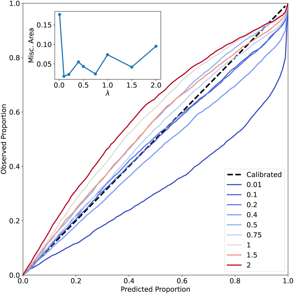 | ||
| Fig. 4 Calibration curves with respect to the hyperparameter λ. The x-axis shows the predicted probability to obtain the correct value for the error in a given percentile, the y-axis shows the true probability. The trend line shows the behavior of a perfectly calibrated model. Inside the plot, the area between the curve and the trend line, also called miscalibration area, is shown as a function of the hyperparameter λ. A smaller miscalibration area indicates a better model. | ||
3.2 Classification of predictions
The effect of bias in the training set for PhysNet-type models was previously found to negatively impact prediction capabilities across chemical space.33 In the context of uncertainty quantification, it is also of interest to understand how the predicted variance can be related to the error in the prediction for an individual prediction. For this, the relationship between the predicted variance and the error of prediction was studied following a classification scheme, see Methods section. To this end, the subset of QM9 used for hyperparameter optimization was considered. Then the molecules in the test set were evaluated with the models trained with different values of the hyperparameter λ.For all the tested models, the largest percentage of molecules (≈80%) was found to be True Negatives (TN), see Fig. 5A. This indicates that the model recognizes for most of the samples that there is sufficient information for a correct prediction. On the other hand, molecules classified as True Positives (TP) correspond to samples for which predictions are difficult. Hence, these molecules lie outside the training distribution because they are associated with large prediction errors and the model is ‘aware’ of this. As expected, the number of TP and FP increases with increasing λ. This is a consequence of the inflation of uncertainty by making the model less confident about its prediction which results in misclassification of molecules because – as described before – the error in the prediction is independent on the value of λ, see Fig. S6.† Finally, the number of False Negative (FN) samples in the data is approximately independent on λ. As described before, the molecules in this category contain information on the boundary of the training distribution which compromises the model's prediction capability. The constant number of FN is indicative of a systematic problem that can only be corrected by providing additional samples of similar molecules. The distribution of FP and FN was further analyzed in Fig. S7.† The results indicate that the categories distribute uniformly over the energies sampled. It is also observed that false negatives (i.e. “underconfident”) tend to be more present at smaller total energy (≈−65 eV) whereas false positives (“overconfident”) are more common for larger total energy (≈−80 eV). Furthermore, the number of FPs decreases rapidly with decreasing value of the hyperparameter λ, whereas for FNs this number is rather insensitive to λ, see also Fig. 5A.
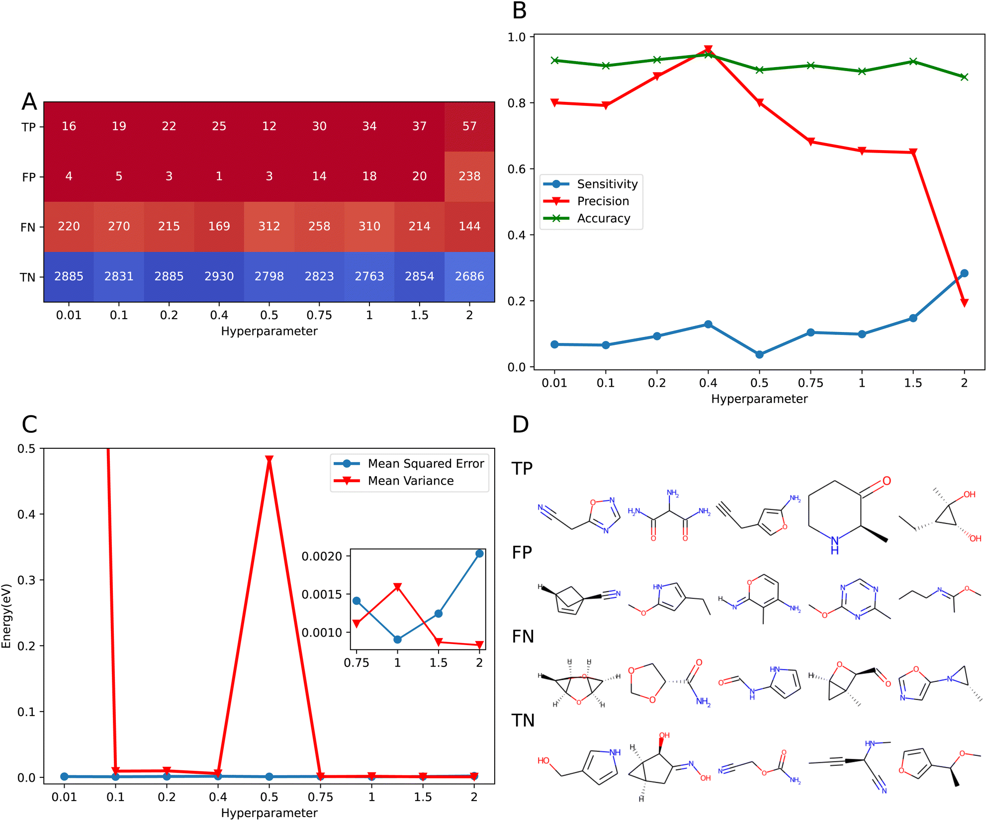 | ||
| Fig. 5 Results of the classification procedure. (A) Confusion matrix with respect to the value of the hyperparameter λ, inside each panel is the number of molecules that belong to the defined categories. The abbreviations refer to TP: True Positive, FP: False Positive, TN: True Negative, and FN: False Negative for information in how those categories are defined consult the Methods section. (B) Accuracy (green, eqn (16)), sensitivity (blue, eqn (17)), and precision (red, eqn (18)) depending on λ. (C) The MSE and MV for the full set of molecules as a function of λ. The mean variance for λ = 0.01 is not shown for clarity. The inset of the plot shows the behavior for λ ≥ 0.75. (D) Chemical structures of the top 5 most common molecules in each of the four classes. | ||
A summary of the relationship between the four classifications in term of model accuracy, sensitivity, and precision is given in Fig. 5B. In all cases the accuracy of the model is appropriate, since the largest part (≈90%) of the studied samples are correctly predicted (i.e. TN) and the variance reflects the prediction error. On the other hand, the precision of the model is also high (≈80%) but starts to decrease as λ increases. In the present context, precision is a measure for the model's capability to recognize ‘problematic’ cases which also correspond to a real deficiency in the model which can be assessed by comparing the prediction with the true value and the predicted variance. It is expected that as the model becomes more underconfident, the precision decreases as there are more molecules misclassified due to inflation of the uncertainty. Conversely, sensitivity describes how many of the molecules that present a problem in the prediction are identified by the model. Here, the sensitivity increases for λ > 0.5: as the model becomes less confident, the probability to detect samples that are truly problematic increases. It should, however, also be pointed out that the numerical values for (ε*, σ*) to define the different categories will impact on how the classifications impact model characteristics such as “precision” or “sensitivity”.
The MV and MSE for the complete set of samples as a function of λ are provided in Fig. 5C. It is found that with the exception of λ = 0.01 and λ = 0.5, MV and MSE are comparable, which is a desired characteristic of the model. However, since it is additionally desirable that MV < MSE the variance obtained by the model accounts for the variance term in eqn (15). Therefore, the difference between MSE and MV is a constant value that corresponds to the combination of the bias of the model and the irreducible error. The advantage of this definition is that the variance can be mainly attributed to the data used for training. This provides a rational basis for further improvement of the training data. It is noted that the condition MV < MSE is only fulfilled for λ = 0.75 and λ > 1.5. A summary with the values of all the metrics tested for calibration is given in Table S1.†
Fig. 5D and S8 to S11† present concrete molecules from each of the four categories. Although the molecules used in the training, validation and test sets were kept constant for the different models, the molecules identified as outliers differed for each value of λ. However, it is instructive to identify molecules that appear more frequently in the various tests. These chemical structures are studied in more detail on the following sections with the aim to identify systematic errors and sampling problems and how they can be corrected.
3.3 Artificial bias experiment
To provide a more chemically motivated analysis of predicted energies and associated variances, a model was trained using the first 25k molecules of QM9. The question addressed is whether predicted energies and variances for molecules not used in the training of the model are more likely to be true positives than for molecules with little coverage in the training set. Since the structures in QM9 were derived from graph enumeration, the order of the molecules in the database already biases certain chemical motifs, such as rings, chains, branched molecules and other features.Fig. 6A reports the Tree MAP (TMAP) projection65 of the entire QM9 database (pink) and the first 25k molecules (blue). TMAP is a dimensionality reduction technique with good locality-preserving properties for high dimensional data such as molecular fingerprints. Analysis of the projection suggests that, as a general structural bias, the first 25k molecules over-represent aromatic heterocyclic, 5- and 6- membered rings, and structures with multiple substituted heteroatoms with regards to the relative probability of other structures also present in QM9.
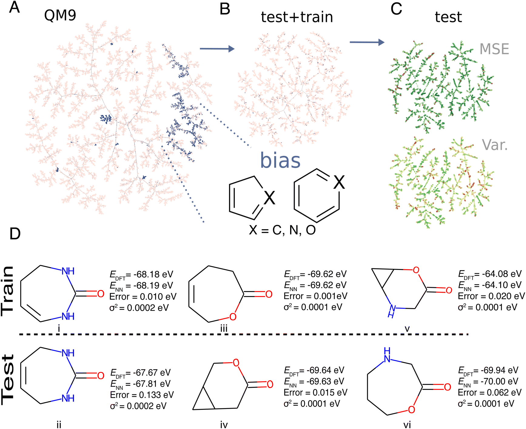 | ||
| Fig. 6 Artificial bias experiment. (A) TMAP of the QM9 database. In blue the structures used for training, the inset shows that the selected part of the database bias the data towards specific chemistry, in this case, aromatic 6- and 5-membered heterocyclic rings scaffolds. In pink, the rest of the structures on QM9. (B) TMAP of the reduced dataset. In pink the structures used for training and validation and in blue the selected random compounds used for test. (C) TMAP of the test set. On top TMAP, for the MSE and down the corresponding for variance. The colormaps which span from the minimum value (green) to 1σ (red). D Pairs of similar molecules (i/ii), (iii/iv), and (v/vi) for which one molecule was in the training set (top) and the related molecule was in the test set (bottom) with reference, prediction and difference energies displayed together with associated variance. | ||
For training the NN, as described in the Methods section, 31500 structures were randomly split (train/validation/test of 0.8/0.1/0.1) and a model with λ = 0.4 was trained to make predictions on the test set. A TMAP projection of the test and train compounds is shown in Fig. 6C. The connectivity of the different tree branches on the TMAP provides information about the local similarity of the molecules where dense regions of the map correspond to clusters of high similarity. The average degree i.e. number of edges between one molecule and its neighbors, for the TNs in the test set – which was the majority class (≈90% of the test samples) – was 2.0 compared with classes FN (169 molecules), TP (25 molecules), and FP (1 molecule) which had average degrees of 1.7, 1.3, 1.0. The lower connectivity for FP compared with TN indicates that “good predictions for the right reason” are more likely if coverage of particular structural and/or chemical motifs is better. Furthermore, it is observed that FPs have a low connectivity which indicates that these molecules are “rare” in the training set. On the other hand, the different sample sizes of the four classes need to be kept in mind when generalizing such conclusions.
The TMAP projection of the test set in Fig. 6B shows the chemical similarity between specific molecules seen during training or testing. In general, molecules identified as TPs contained common scaffolds seen during training in combination with unusual substituents. For example, the moiety of imidazole (a five-membered 1,3-C3N2 ring) was a common fragment in the training set and lies in the biased region of chemical space depicted in Fig. 6A. Common true positives contained this imidazole scaffold inside uncommon fused three ring systems. When the model makes predictions for compounds close in chemical space to molecules of which it has seen diverse examples in the training set, the estimates of variance appear to be more reliable.
Fig. 6D reports three examples of false positives (i.e. molecules with high error and low predicted variance) in the test set. The molecules in the training set are labelled as (i), (iii) and (v), whereas those used for prediction from the test set were (ii), (iv) and (vi). The pair (i/ii) consists of a diazepane core that goes through a double bond migration. Although the rest of the structure is conserved for (i) and (ii), the error in the prediction for molecule (ii) (test) is ≈0.1 eV, but the predicted variance is the same for molecules (i) and (ii). A possible explanation is that the model recognizes that (i) and (ii) are similar which leads to assigning a small variance to (ii). However, this contrasts with the energy difference between molecules i and ii which is ≈0.5 eV.
Pair (iii/iv) involves an oxepane ring with a carbonyl (iii) which is in the training set and the prediction is for an oxabicycloheptane (iv). In this case the model predicts the energy with an error of 0.015 eV. Hence, for pair (iii/iv) the information that the model has from molecule (iii), in addition to the significant presence of bicycles in the training set, makes it easier to predict the energy for molecule iv. Finally, pair (v/vi) is opposite to (iii/iv): training on an Oxa-azabicycloheptane for predicting an Oxazepane. The error for this prediction is considerably higher (≈0.06 eV). This shows that it is easier for the NN to predict bicycles than seven-membered rings and reflects the fact that there are more bicycles in the training set than seven-membered rings. An intriguing aspect of the totality of molecules shown in Fig. 6D is that they all have the same number of heavy atoms, and that they share multiple structural and bonding motifs. This may be the reason why the model assigns a small variance to all of them because the NN is primed to make best use of structural information at the training stage. However, additional tests are required to further generalize this.
Similarly, cases where a ring was expanded or contracted by a single atom between molecules in the training and test set commonly resulted in similar failure modes due to over-confidence. This observation is particularly interesting because it suggests that the model might be overconfident when predicting compounds it has seen sparse but highly similar examples of during training. Uncertainty quantification, in this conception, is effective at predicting in-distribution errors, however, out-of-distribution errors are not as easily quantified by this model.
3.4 Tautomerization set
As a concrete chemical application of how uncertainty quantification can be used, the prediction of energy of tautomer pairs was considered. Tautomerization is a form of reversible isomerization involving the rearrangement of a charged leaving group within a molecule.66 The structures of the molecules involved in a tautomeric pair (A/B) only differ little which makes this an ideal application for the present developments. For the study of tautomeric pairs, three NN models with different values of λ = 0.2, 0.4, 0.75 were trained with QM9 database as described on the Methods section. The test molecules considered come from the Tautobase database.61 For the purpose of this work, only molecules with less than nine heavy atoms (C, N and O) were tested. A total of 442 pairs (884 molecules) was evaluated.The training of PhysNet involves learning of the Atomic Embeddings (AtE) and the centers and widths of the Radial Basis Functions (RBF). These features encode the chemical environment around each atom and therefore contain the “chemical information” about a molecule. This opens the possibility to further analyze the potential relationship contained in the learned parameters to the information about the chemical space contained in the training dataset and how it compares with the chemical space of the test molecules that are the target for prediction. Hence, for the following the mean distances between each of the tested molecules and the molecules in the training set of the database for 〈AtE〉 and 〈RBF〉 were determined according to the procedure described in Section 1 of the ESI.†Fig. 7 shows the results for the relationship between the mean distance of the AtE and RBF, the error, variance and number of atoms for the molecules in the tautobase.
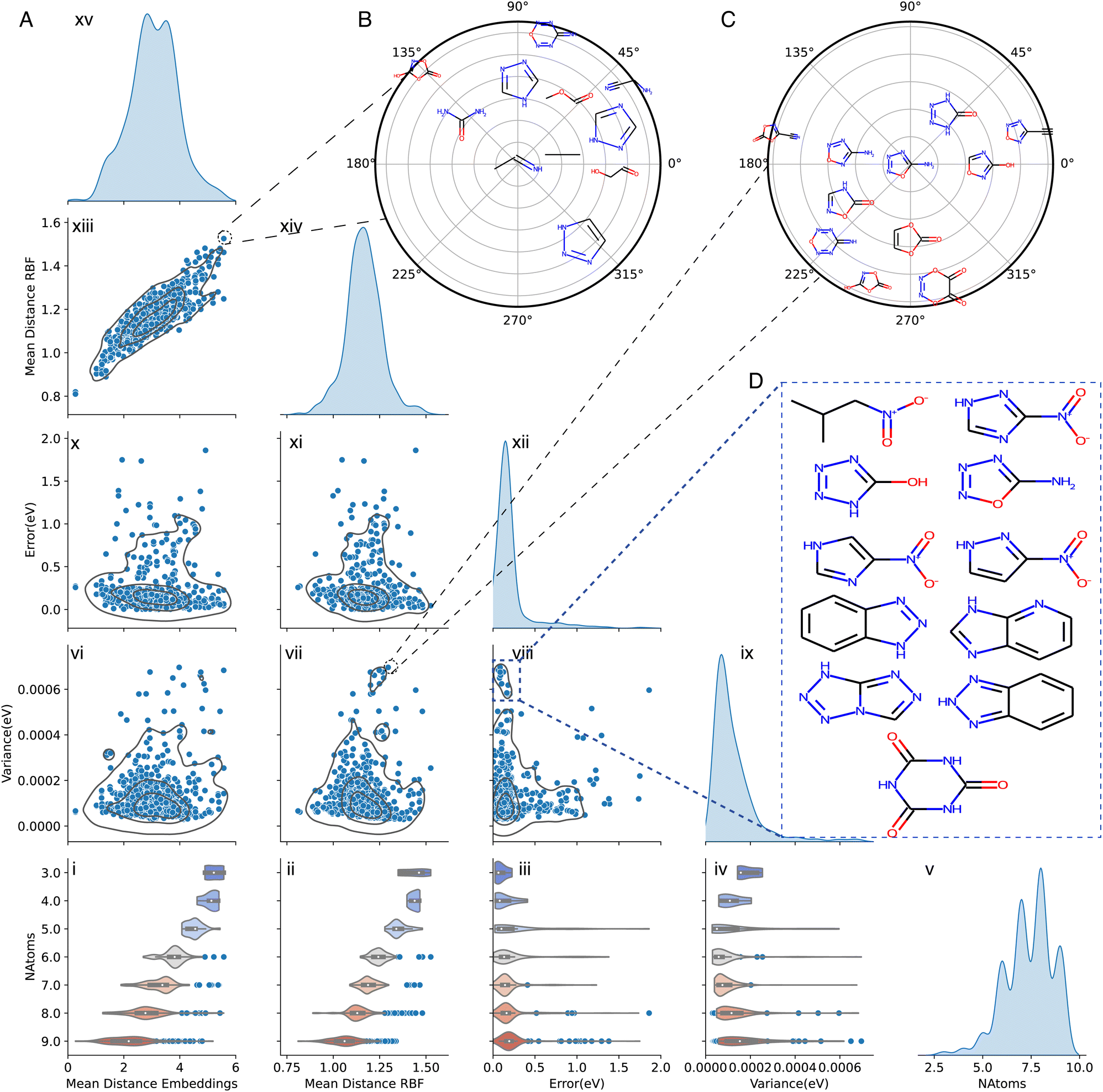 | ||
| Fig. 7 (A) Overview of the comparison between different results for the evaluation of molecules on the tautobase for λ = 0.75 up to the 95th percentile. The diagonal of the Fig. shows the kernel density estimate of the considered properties (mean distance embeddings, mean distance RBF, error (in eV), variance (in eV) and number of atoms). For each of the panels a correlation plot between the variable and a 2D kernel density estimate is shown. On the last row, violin plots for the different considered properties with respect to the number of atoms is shown. Similar plots for λ = 0.2 and λ = 0.4 can be found in the ESI.† (B) Radial plot of the ten closest molecules of the training set on feature space for the molecule in tautobase with the largest distance in embedding and RBF space. (C) Radial plot of the ten closest molecules for the molecule in tautobase with the largest predicted variance and the largest distance in RBF space. (D) Examples of molecules with large predicted variance and small error. Enlarged views of panels (B) and (C) are provided in Fig. S14 and S16†. | ||
The bottom row of Fig. 7A (panels i to v) report 〈AtE〉 and 〈RBF〉, the prediction errors and associated variances sorted by the number of heavy atoms N = 3 to 9 together with the distribution P(N). The dependence of 〈AtE〉 and 〈RBF〉 on N shows that with decreasing number of heavy atoms the mean distance with respect to the molecules with the same number of atoms increases (Fig. 7A(i and ii)). Additionally, the violin plots in Fig. 7A(i and ii) show that the mean distance values are more spread as the number of atoms increases. One explanation for these results is that the available chemical space to explore increases with N which is also reflected in the number of samples with a given number of heavy atoms in the training dataset; consequently, the distance between the molecules with a low number of atoms increases. In other words, a larger molecule explores chemical space more extensively in terms of chemical environments, atom types, bonding patterns and other characteristics of chemical space. The relationship between error and the number of atoms illustrates how the smaller mean distance in RBF and AtE leads to a smaller error. Furthermore, the number of outliers also scales with the size of the molecules. Comparing error and variance by the number of heavy atoms, it is clear that for up to 5 atoms they behave similarly (Fig. 7A(iii and iv)). From Fig. 7A(iii), it is clear that the error distribution shifts with increasing number of atoms in the molecule. The center of mass of the predicted variance distribution, (see Fig. 7A(iv)) is initially at a high value and progressively decreases until 5 heavy atoms and then to increase again. It should be noted that the number of outliers for error and variance increases with the number of heavy atoms which affects the displacement on the center of mass. Finally, the spread of error and variance by the number of atoms (Fig. 7A(iii and iv)) presents similar shapes up to 8 heavy atoms. For molecules with 8 and 9 atoms, the variance is more spread out whereas the error distribution is more compact.
Panels vi, vii, x, and xi in Fig. 7A show that variance and error are similarly distributed depending on 〈AtE〉 and 〈RBF〉, respectively. For the entire range of 〈AtE〉 and 〈RBF〉 low variance (<0.0002 eV) and low prediction errors (<0.25 eV) are found. Increased variance (≈0.0005 eV) is associated with both, larger 〈AtE〉 and 〈RBF〉 whereas larger prediction errors (>1.0 eV) are found for intermediate to large 1.0 ≤ 〈RBF〉 ≤ 1.5. This similarity is also reflected in a near-linear relationship between 〈AtE〉 and 〈RBF〉 reported in panel (xiii) of Fig. 7A.
Prediction error and variance are less well correlated for the evaluated molecules from tautobase, see panel (viii) of Fig. 7A. This can already be anticipated when comparing panels (i) and (ii). With increasing N, the position of the maximum error shifts monotonously to larger values whereas the variance is higher for N = 3, decreases until N = 6, after which it increases again. Hence, for tautobase and QM9 as the reference data, base error and variance are not necessarily correlated.
To gain a better understanding of the prediction performance of QM9 for molecules in the Tautobase from the point of view of feature space, polar plots considering extreme cases were constructed, see ESI† for technical details. Fig. 7B shows the case for the molecule (center) with the largest average distance in RBF and AtE for molecules with the same number of atoms used for training for this representation; only the ten closest neighbours are shown. Although the molecule is relatively simple, no structure in the training set contains sufficient and appropriate information for a correct prediction. Despite abundant information about similar chemical environments but with different spatial arrangements, combination with different functional groups or different bonding arrangements, potentially conflicting information in the training set leads to uncertainties in the prediction. A second example, that of the molecule with largest variance and largest distance in RBF, is shown in Fig. 7C. As for molecule ii in Fig. 6D this case also highlights how seemingly small changes in bonding pattern, functional groups and atom arrangements can lead to large errors. However, in this case the abundant and similar structural information in the training set leads to a large predicted variance. In other words, “redundancy” in the training set can lead to vulnerabilities in the trained model as was previously found for predictions based on training with the ANI-1 database compared with the much smaller ANI-1E set: despite its larger size, predictions based on ANI-1 were less accurate than those based on ANI-1E.33
As a final example of the relationship between error and variance, the chemical structures for a set of molecules with low error but high variance is highlighted in Fig. 7D and shows that heterocyclic rings and bicycles are well covered in the training set. An interesting aspect is that molecules with a nitro-group (–NO2) appear with high variance and low error. This effect can be rationalized by considering the design of the GDB-17 Database67 which is the source of the QM9 set: for GDB-17 aliphatic nitro groups were excluded, but aromatic nitro groups were retained. Therefore, the trained model will have similar information based on structural considerations but the quality of the data in view of a molecules' energetics is low which leads to significant variance.
Finally, it is of interest to analyze tautomer pairs (A/B) for which the difference in the predicted variance is particularly large. Fig. 8A reports the distribution p(σ2A − σ2B) for trained models with different values of the hyperparameter λ. First, it is found that the distribution of variance differences depends on the value of λ. Therefore, particularly prominent outliers can be avoided by careful evaluation of the predictions. Secondly, large differences (star in Fig. 8A) in the variances can occur and indicate that the trained models are particularly uncertain in their prediction. To illustrate this, three tautomer pairs were identified and are analyzed in more detail in the following. For molecules B1 to B3 it is found that their functional groups are not present or are poorly represented in QM9. These include the N![[double bond, length as m-dash]](https://www.rsc.org/images/entities/char_e001.gif) O nitro group in an aliphatic chain (B3), vinyl alcohol (B1), and hydroxyl imine (B2, only one representative in QM9). Furthermore, the pair (A3/B3) is zwitterionic.
O nitro group in an aliphatic chain (B3), vinyl alcohol (B1), and hydroxyl imine (B2, only one representative in QM9). Furthermore, the pair (A3/B3) is zwitterionic.
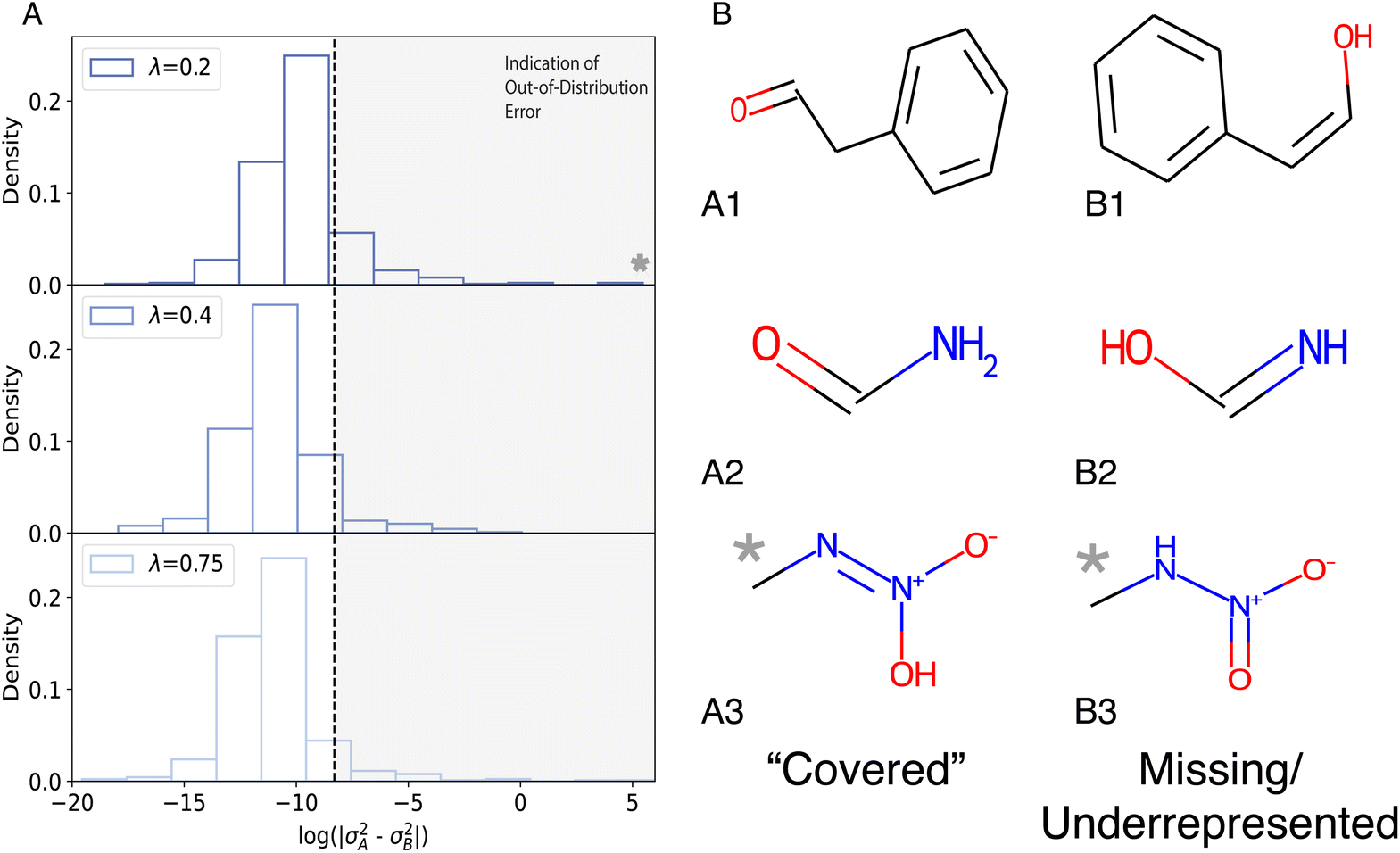 | ||
| Fig. 8 (A) The log distribution of differences in predicted variance between tautomer pairs, A (low variance) and B (high variance). (B) Tautomer pairs (A/B) containing chemical groups, nitro and vinyl alcohols, outside the training set (B1-3) are easily identified. The imine group in B2 was present in only one molecule in the training set. Numerical values for energies and variances are summarized in Table 1. | ||
| Molecule | E DFT | E NN | σ 2 | ||||
|---|---|---|---|---|---|---|---|
| λ | 0.2000 | 0.4000 | 0.7500 | 0.2000 | 0.4000 | 0.7500 | |
| A1 | −79.8900 | −79.6800 | −79.6900 | −79.6800 | 0.0018 | 0.0002 | 0.0002 |
| Δ | 0.2100 | 0.2000 | 0.2100 | ||||
| B1 | −79.5900 | −79.2800 | −79.4400 | −79.3600 | 0.0249 | 0.0002 | 0.0002 |
| Δ | 0.3100 | 0.1500 | 0.2300 | ||||
| A2 | −23.5900 | −23.5200 | −23.5200 | −23.5200 | 0.0016 | 0.0012 | 0.0002 |
| Δ | 0.0700 | 0.0700 | 0.0700 | ||||
| B2 | −23.0200 | −22.7500 | −22.8800 | −22.9100 | 0.0019 | 0.0011 | 0.0007 |
| Δ | 0.2700 | 0.1400 | 0.1100 | ||||
| A3 | −30.8600 | −32.6700 | −32.5800 | −32.2000 | 0.0046 | 0.0004 | 0.2243 |
| Δ | 1.8100 | 1.7200 | 1.3400 | ||||
| B3 | −31.6300 | −32.0200 | −32.0800 | −32.6900 | 229.6200 | 0.0035 | 0.0033 |
| Δ | 0.3900 | 0.4500 | 1.0600 | ||||
As is shown in Fig. 8B the chemical motifs and functional groups in A1 to A3 are covered by QM9 whereas those in their tautomeric twins (B1 to B3) are not. For molecule B1 (vinyl alcohol) examples are entirely absent in QM9 and the presence of hydroxyl groups bound to sp2 (aromatic) carbons is not sufficient for a reliable prediction for B1. It is also noted that the difference Δ between the target energy (EDFT) and the predictions (ENN) are largely independent on λ for A1 but differ by a factor of two for B1. This is also observed for the pair (A2/B2) for which the uncertainties are more comparable than for (A1/B1).
Finally, the pair (A3/B3) poses additional challenges. First, the variance for one value of λ for B3 is very large and for A3 one of the variances is also unusually large, given that similar examples to A3 are part of the training set. Secondly, although A3 is better represented in the training set, the difference between target value and prediction is larger than 1 eV for all models. These observations are explained by the fact that (A3/B3) are both zwitterionic and the uncertainty associated with B3 may in part be related to the fact that QM9 only contains few examples of sp2 NO bonds except for a small number of heterocyclic rings which are chemically dissimilar compounds compared with B3. Furthermore, for B3 some of the atom–atom separations (“bond lengths”) are poorly covered by QM9. For the N–N distance, the QM9 database contains the range from 1.2 Å to 1.4 Å (see Fig. S17†) whereas N–N in B3 is 1.383 Å which is a low probability region for p(rNN). This is also the case for compound A3 although p(rNN) has a local maximum at the corresponding N–N separation. In conclusion, the majority of prediction problems in Fig. 8B can be related to origins in the underlying chemistry. Interestingly, even a careful analysis of the performance of a trained model on the training set (see compound A3) may provide insight into coverage and potential limitations when making predictions from the trained model.
4 Discussion and conclusions
The present work introduces uncertainty quantification for the prediction of total energies and variances for molecules based on a trained atomistic neural network. The approach is generic and it is expected that it can be generalized to other NN-architectures and observables.With respect to computational effort it is noted that the current approach requires training of several independent models for a range of values for the hyperparameter λ. However, the uncertainty on a prediction can be obtained from evaluating a single model. This is an advantage compared to ensemble models which require the evaluation of all trained models to obtain an estimate of the uncertainty. For ensemble-based approaches the statistical error of a prediction 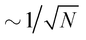 whereas for DER considered here this is not the case. Rather, a number of models needs to be trained for calibration but as demonstrated here, N = 10 is a meaningful estimate for this. On the other hand, Bayesian methods rapidly become impractical for larger data sets as already mentioned in the Introduction. One possible way to avoid training for a range of λ – values is to use recalibration methods.53,68 However, such methods are quite new and still need to be validated by different metrics. Finally, the results obtained here can be used as a starting point for model training on other databases but it remains to be seen if the calibration results are transferable to other databases.
Data completeness and quality directly impact the forecasting capabilities of statistical models. Although quantum chemical models are trained, for example, on total energies of a set of molecules, it is not evident how to select the best suitable training set for most accurately predicting energy differences between related compounds, such as structural isomers as demonstrated in this work. PhysNet-DER is a step towards the design of validated, well-defined databases containing meaningful information (“smart data”).27–29 In this process one also anticipates that targeted databases will become available for specific applications in chemistry, such as tautomerization energies, hydration energies, or HOMO–LUMO gaps, to name a few. Also, the findings from the present work will be useful to be employed together with established methods like Gaussian process approximation.39
A large part of the present work was concerned with the impact of redundant/missing information in the databases used to train a model on the prediction of specific properties in chemical space. The results confirm that redundancies can impact heavily the prediction of a property and its variance. However, it is still necessary to systematically identify and remove conflicting information while retaining training quality. In this regard, the combination of unsupervised machine learning methods69–72 with the approach introduced here will hopefully allow to design workflows to broadly explore chemical space at low computational cost. Another point that requires attention is the underlying assumption in many similar applications that the predicted property can be represented as a normal (Gaussian) distribution. The present and earlier studies73 indicate that this assumption is only valid approximately.
It was noted in Fig. S2† that the average predicted variance for a hold-out set of molecules decreased with increasing training set size until a certain point. Beyond that, models trained on the most extensive training corpus predicted higher variance. This is consistent with the expectation that as new molecules are introduced to the training set, the probability of adding previously unseen information is initially large, but decreases as the training set grows. This is indicative of the law of diminishing returns.74 The artificial bias experiment carried out here suggests that the model may become sensitive to redundant information which leads to overconfident estimates of variance for over-represented chemical motifs at the expense of being under-confident for motifs with fewer training examples. The observation that larger training sets can introduce higher uncertainties is compelling and highlights the need for a deeper understanding of the role of bias when evaluating atomistic neural networks for predictions made across chemical space.
Distances in the embedding space (AtE/RBF) of the neural network were studied to visualize and analyze the proximity between molecules in the training and test set, see Fig. S14 and S16.† This allowed to assess how similar molecules can influence the prediction by making the model less confident. On the other hand, it was also possible to recognize molecules for which insufficient information was available in the database for a prediction. In other words, analysis of the embedding space also hinted towards the role of similar information on model degradation. It is of interest to note that analysis of the embedding space was previously done for uncertainty determination.36,43 As used in the present work, distances in embedding space provide a qualitative picture for what information influences a prediction. This can be used in a more targeted fashion for model improvement but more systematic studies for this natural next step are required.
Some of the essential findings of the present work concern the notion that single metrics are not particularly meaningful to judge the calibration of a trained model. Exploration and development of meaningful metrics will benefit evidence-based inference.75 Also, it is not always true that error and variance are directly related which is counter typical expectations in statistical learning. It is also demonstrated that mean variance and mean squared error can behave in counter-intuitive ways which points towards deficiencies in the assumed posterior distribution.
As found here, uncertainty quantification is essential and reveals that the nature and coverage of the training set used for model construction plays an important role when applied to specific chemical tasks. For example, it is demonstrated for tautomerization energies that classification of predictions can be used to identify problematic cases at the prediction stage. Furthermore, it was found that similar information in low quantity returns low uncertainties but high errors, whereas similar information in large quantities results in small errors but high predicted uncertainties. A notable example of this is the nitro group in the training database, which is not present for aliphatic chains but for aromatic rings. Thus, for a balanced ML-based model for chemical exploration an equilibrium between the quantity and the quality of data in the database is required. The information from UQ can be used in the future to build targeted and evidence-based datasets for a broad range of chemical observables based on active learning strategies and for constructing robust high-dimensional potential energy surfaces of molecules.
Data availability
The code for the new PhysNet-DER model can be found at: https://github.com/LIVazquezS/PhysNet_DER and https://github.com/MMunibas/PhysNet_DER.Author contributions
Design of research: LIVS, EDB, MM; performing research: LIVS, EDB; software development: LIVS; new analytic tools: LIVS; data analysis and interpretation: LIVS, EDB, MM; manuscript writing: LIVS, EDB, MM.Conflicts of interest
There are no conflicts to declare.Acknowledgements
The authors acknowledge financial support from the Swiss National Science Foundation (NCCR-MUST and Grant No. 200021-7117810, to MM) and the University of Basel. LIVS acknowledges fruitful discussions with Dr Kai Töpfer and Dr Oliver Unke.Notes and references
- M. Meuwly, Chem. Rev., 2021, 121, 10218–10239 CrossRef PubMed.
- K. Töpfer, S. Käser and M. Meuwly, Phys. Chem. Chem. Phys., 2022, 24, 13869–13882 RSC.
- F. Noé, S. Olsson, J. Köhler and H. Wu, Science, 2019, 365, eaaw1147 CrossRef PubMed.
- S. Manzhos and T. Carrington Jr, Chem. Rev., 2020, 121, 10187–10217 CrossRef PubMed.
- D. Koner and M. Meuwly, J. Chem. Theory Comput., 2020, 16, 5474–5484 CrossRef CAS.
- R. Conte, C. Qu, P. L. Houston and J. M. Bowman, J. Chem. Theory Comput., 2020, 16, 3264–3272 CrossRef CAS.
- O. T. Unke, S. Chmiela, H. E. Sauceda, M. Gastegger, I. Poltavsky, K. T. Schütt, A. Tkatchenko and K.-R. Müller, Chem. Rev., 2021, 121, 10142–10186 CrossRef CAS.
- O. T. Unke, M. Stöhr, S. Ganscha, T. Unterthiner, H. Maennel, S. Kashubin, D. Ahlin, M. Gastegger, L. M. Sandonas, A. Tkatchenko, et al., arXiv preprint arXiv:2205.08306, 2022.
- D. Schwalbe-Koda and R. Gómez-Bombarelli, Machine Learning Meets Quantum Physics, Springer, 2020, pp. 445–467 Search PubMed.
- B. Huang and O. A. von Lilienfeld, Chem. Rev., 2021, 121, 10001–10036 CrossRef CAS PubMed.
- P. Ramos-Sánchez, J. N. Harvey and J. A. Gámez, J. Comput. Chem., 2022, 1 DOI:10.1002/jcc.27011.
- K. T. Schütt, H. E. Sauceda, P.-J. Kindermans, A. Tkatchenko and K.-R. Müller, J. Chem. Phys., 2018, 148, 241722 CrossRef PubMed.
- J. S. Smith, O. Isayev and A. E. Roitberg, Chem. Sci., 2017, 8, 3192–3203 RSC.
- X. Gao, F. Ramezanghorbani, O. Isayev, J. S. Smith and A. E. Roitberg, J. Chem. Inf. Model., 2020, 60, 3408–3415 CrossRef CAS PubMed.
- T. W. Ko, J. A. Finkler, S. Goedecker and J. Behler, Nat. Commun., 2021, 12, 1–11 CrossRef.
- O. T. Unke, S. Chmiela, M. Gastegger, K. T. Schütt, H. E. Sauceda and K.-R. Müller, Nat. Commun., 2021, 12, 1–14 CrossRef PubMed.
- J. A. Keith, V. Vassilev-Galindo, B. Cheng, S. Chmiela, M. Gastegger, K.-R. Müller and A. Tkatchenko, Chem. Rev., 2021, 121, 9816–9872 CrossRef.
- P. Domingos, Commun. ACM, 2012, 55, 78–87 CrossRef.
- H. Sanders and J. Saxe, Proceedings of Blackhat, 2017, 2017 Search PubMed.
- M. F. Kilkenny and K. M. Robinson, Health Inf. Manag. J., 2018, 47, 103–105 Search PubMed.
- G. Canbek, Wiley Interdiscip. Rev. Data Min. Knowl. Discov., 2022, 12, e1456 Search PubMed.
- R. L. Tweedie, K. L. Mengersen and J. A. Eccleston, Chance, 1994, 7, 20–27 CrossRef.
- C. Babbage, Passages from the Life of a Philosopher, Cambridge University Press, 2011 Search PubMed.
- R. S. Geiger, D. Cope, J. Ip, M. Lotosh, A. Shah, J. Weng and R. Tang, Quant. sci. stud., 2021, 2, 795–827 CrossRef.
- J. C. Weyerer and P. F. Langer, Proceedings of the 20th Annual International Conference on Digital Government Research, 2019, pp. 509–511 Search PubMed.
- B. Saha and D. Srivastava, 2014 IEEE 30th international conference on data engineering, 2014, pp. 1294–1297 Search PubMed.
- F. Iafrate, Digital Enterprise Design & Management, Springer, 2014, pp. 25–33 Search PubMed.
- M. T. Baldassarre, I. Caballero, D. Caivano, B. Rivas Garcia and M. Piattini, Proceedings of the 1st ACM SIGSOFT International Workshop on Ensemble-Based Software Engineering, 2018, pp. 19–24 Search PubMed.
- I. Triguero, D. García-Gil, J. Maillo, J. Luengo, S. García and F. Herrera, Wiley Interdiscip. Rev. Data Min. Knowl. Discov., 2019, 9, e1289 Search PubMed.
- O. A. Von Lilienfeld, Angew. Chem., Int. Ed., 2018, 57, 4164–4169 CrossRef CAS PubMed.
- S. Heinen, M. Schwilk, G. F. von Rudorff and O. A. von Lilienfeld, Mach. Learn. Sci. Technol., 2020, 1, 025002 CrossRef.
- S. Käser, D. Koner, A. S. Christensen, O. A. von Lilienfeld and M. Meuwly, J. Phys. Chem. A, 2020, 124, 8853–8865 CrossRef PubMed.
- L. I. Vazquez-Salazar, E. D. Boittier, O. T. Unke and M. Meuwly, J. Chem. Theory Comput., 2021, 17, 4769–4785 CrossRef CAS.
- S. Käser, O. T. Unke and M. Meuwly, New J. Phys., 2020, 22, 055002 CrossRef.
- S. Käser, J. O. Richardson and M. Meuwly, arXiv preprint arXiv:2208.01315, 2022.
- J. P. Janet, C. Duan, T. Yang, A. Nandy and H. J. Kulik, Chem. Sci., 2019, 10, 7913–7922 RSC.
- P. Zheng, W. Yang, W. Wu, O. Isayev and P. O. Dral, J. Phys. Chem. Lett., 2022, 13, 3479–3491 CrossRef.
- F. Musil, M. J. Willatt, M. A. Langovoy and M. Ceriotti, J. Chem. Theory Comput., 2019, 15, 906–915 CrossRef PubMed.
- V. L. Deringer, A. P. Bartók, N. Bernstein, D. M. Wilkins, M. Ceriotti and G. Csányi, Chem. Rev., 2021, 121, 10073–10141 CrossRef PubMed.
- J. Gawlikowski, C. R. N. Tassi, M. Ali, J. Lee, M. Humt, J. Feng, A. Kruspe, R. Triebel, P. Jung, R. Roscheret al., arXiv preprint arXiv:2107.03342, 2021.
- M. Abdar, F. Pourpanah, S. Hussain, D. Rezazadegan, L. Liu, M. Ghavamzadeh, P. Fieguth, X. Cao, A. Khosravi and U. R. Acharya, et al. , Inf. Fusion, 2021, 76, 243–297 CrossRef.
- A. Malinin, S. Chervontsev, I. Provilkov and M. Gales, arXiv preprint arXiv:2006.11590, 2020.
- L. Hirschfeld, K. Swanson, K. Yang, R. Barzilay and C. W. Coley, J. Chem. Inf. Model., 2020, 60, 3770–3780 CrossRef CAS PubMed.
- A. Amini, W. Schwarting, A. Soleimany and D. Rus, Advances in Neural Information Processing Systems, 2020, pp. 14927–14937 Search PubMed.
- A. P. Soleimany, A. Amini, S. Goldman, D. Rus, S. N. Bhatia and C. W. Coley, ACS Cent. Sci., 2021, 7, 1356–1367 CrossRef CAS.
- O. T. Unke and M. Meuwly, J. Chem. Theory Comput., 2019, 15, 3678–3693 CrossRef CAS PubMed.
- A. Paszke, S. Gross, F. Massa, A. Lerer, J. Bradbury, G. Chanan, T. Killeen, Z. Lin, N. Gimelshein, L. Antiga, A. Desmaison, A. Kopf, E. Yang, Z. DeVito, M. Raison, A. Tejani, S. Chilamkurthy, B. Steiner, L. Fang, J. Bai and S. Chintala, Adv. Neural Inf. Process Syst., 2019, 32, 8024–8035 Search PubMed.
- D. P. Kingma and J. Ba, arXiv preprint arXiv:1412.6980, 2014.
- D. Levi, L. Gispan, N. Giladi and E. Fetaya, arXiv preprint arXiv:1905.11659, 2019.
- K. Tran, W. Neiswanger, J. Yoon, Q. Zhang, E. Xing and Z. W. Ulissi, Mach. learn.: sci. technol., 2020, 1, 025006 Search PubMed.
- J. Busk, P. B. Jørgensen, A. Bhowmik, M. N. Schmidt, O. Winther and T. Vegge, Mach. learn.: sci. technol., 2021, 3, 015012 Search PubMed.
- V. Kuleshov, N. Fenner and S. Ermon, International conference on machine learning, 2018, pp. 2796–2804 Search PubMed.
- Y. Chung, I. Char, H. Guo, J. Schneider and W. Neiswanger, arXiv preprint arXiv:2109.10254, 2021.
- P. Pernot, J. Chem. Phys., 2022, 156, 114109 CrossRef PubMed.
- L. Kahle and F. Zipoli, Phys. Rev. E, 2022, 105, 015311 CrossRef PubMed.
- K. Cheng, F. Calivá, R. Shah, M. Han, S. Majumdar and V. Pedoia, Medical Imaging with Deep Learning, 2020, pp. 121–135 Search PubMed.
- T. Hastie, R. Tibshirani, J. H. Friedman and J. H. Friedman, The elements of statistical learning: data mining, inference, and prediction, Springer, 2009 Search PubMed.
- M. J. Schervish and M. H. DeGroot, Probability and statistics, Pearson Education London, UK, 2014 Search PubMed.
- J. Watt, R. Borhani and A. K. Katsaggelos, Machine learning refined: Foundations, algorithms, and applications, Cambridge University Press, 2020 Search PubMed.
- O. Wahl and T. Sander, J. Chem. Inf. Model., 2020, 60, 1085–1089 CrossRef PubMed.
- L. I. Vazquez-Salazar and M. Meuwly, QTautobase: A quantum tautomerization database, 2021, DOI:10.5281/zenodo.4680972.
- B. Ruscic, Int. J. Quantum Chem., 2014, 114, 1097–1101 CrossRef.
- G. Scalia, C. A. Grambow, B. Pernici, Y.-P. Li and W. H. Green, J. Chem. Inf. Model., 2020, 60, 2697–2717 CrossRef CAS PubMed.
- K. Schutt, P. Kessel, M. Gastegger, K. Nicoli, A. Tkatchenko and K.-R. Müller, J. Chem. Theory Comput., 2018, 15, 448–455 CrossRef PubMed.
- D. Probst and J.-L. Reymond, J. Cheminf., 2020, 12, 12 Search PubMed.
- A. Wilkinson and A. McNaught, IUPAC Compendium of Chemical Terminology (the “Gold Book”), International Union of Pure and Applied Chemistry, Zürich, Switzerland, 1997 Search PubMed.
- L. Ruddigkeit, R. Van Deursen, L. C. Blum and J.-L. Reymond, J. Chem. Inf. Model., 2012, 52, 2864–2875 CrossRef CAS PubMed.
- G. Palmer, S. Du, A. Politowicz, J. P. Emory, X. Yang, A. Gautam, G. Gupta, Z. Li, R. Jacobs and D. Morgan, npj Comput. Mater., 2022, 8, 1–9 CrossRef.
- P.-A. Cazade, W. Zheng, D. Prada-Gracia, G. Berezovska, F. Rao, C. Clementi and M. Meuwly, J. Chem. Phys., 2015, 142, 01B6101 Search PubMed.
- M. Ceriotti, J. Chem. Phys., 2019, 150, 150901 CrossRef PubMed.
- A. Glielmo, B. E. Husic, A. Rodriguez, C. Clementi, F. Noé and A. Laio, Chem. Rev., 2021, 121, 9722–9758 CrossRef CAS.
- G. Fonseca, I. Poltavsky, V. Vassilev-Galindo and A. Tkatchenko, J. Chem. Phys., 2021, 154, 124102 CrossRef CAS.
- O. T. Unke and M. Meuwly, J. Chem. Phys., 2018, 148, 241708 CrossRef PubMed.
- A. V. Joshi, in Essential Concepts in Artificial Intelligence and Machine Learning, Springer International Publishing, Cham, 2020, pp. 9–20 Search PubMed.
- M. Naser and A. H. Alavi, Archit. Struct. and Const., 2021, 1–19 Search PubMed.
Footnote |
| † Electronic supplementary information (ESI) available: Details of the calculation of mean distance between molecules of test set and the training set in feature space, construction of polar plots. See DOI: https://doi.org/10.1039/d2sc04056e |
| This journal is © The Royal Society of Chemistry 2022 |