 Open Access Article
Creative Commons Attribution 3.0 Unported Licence
Quantum circuit learning as a potential algorithm to predict experimental chemical properties†
Kan
Hatakeyama-Sato
 *a,
Yasuhiko
Igarashi
b,
Takahiro
Kashikawa
c,
Koichi
Kimura
c and
Kenichi
Oyaizu
 *a
*a
aDepartment of Applied Chemistry, Waseda University, Tokyo 169-8555, Japan. E-mail: satokan@toki.waseda.jp; oyaizu@waseda.jp
bFaculty of Engineering, Information and Systems, University of Tsukuba, 1-1-1 Tennodai, Tsukuba 305-8573, Japan
cFujitsu Ltd, Kanagawa 211-8588, Japan
First published on 2nd December 2022
Abstract
We introduce quantum circuit learning (QCL) as an emerging regression algorithm for chemo- and materials-informatics. The supervised model, functioning on the rule of quantum mechanics, can process linear and smooth non-linear functions from small datasets (<100 records). Compared with conventional algorithms, such as random forest, support vector machine, and linear regressions, the QCL can offer better predictions with some one-dimensional functions and experimental chemical databases. QCL will potentially help the virtual exploration of new molecules and materials more efficiently through its superior prediction performances.
1 Introduction
Recent data-oriented science provides chemical and material research insights by treating versatile experimental data with statistical tools.1–5 Compared to human-based data recognition and accumulation, experimental data are analyzed and stored more objectively by data science.1,3 Such a data-oriented approach offers a more solid platform for interdisciplinary research conducted by chemists, data scientists, physicists, and experts in any other fields.3,5Evaluating molecular and material properties is essential in materials and chemo-informatics.4,5 Various supervised models, trained to predict specific properties from explanatory variables by learning their statistical relationships, have been developed in machine learning.5 There are many supervised models represented by linear algorithms, support vector machines, and decision tree-based ensembles.5 Also, recent deep learning technology of neural networks has broken the limit of prediction accuracy by drastically increasing the model complexity.6 In chemical and material fields, appropriate use of such supervised models afforded the prediction of versatile material and chemical properties, such as conductivity,7,8 energy level,9 photoconversion efficiency,10 and toxicity.4 Their prediction accuracy can exceed human experts and traditional computational simulations, gradually forming a solid platform for data-oriented science.4,5,8–10
On the other hand, most data science projects still have difficulty with the reliable prediction of experimental properties. The main challenges are (a) the lack of trainable records and (b) complex molecular interactions. Due to the high cost of actual experiments, typical database sizes of material projects are around 101–102,7 whereas deep learning mainly targets databases with over 104 records.4–6 Although recent deep learning approaches, represented by fine-tuning (transfer learning) and multipurpose learning, may offer an opportunity for small datasets, they may not be the complete solutions due to the still insufficient and diverse material databases to learn.2,7,11
As a promising approach, sparse modeling aims to extract linearity between explanatory and target variables.12,13 The method is powerful against small datasets owing to the simple linear assumption, and successful data analyses have been reported.12,14 Still, material and chemical properties appear from complex, non-linear atomic interactions.5,8 The linear approximation would face difficulties in expressing the non-linear system.
Here, we introduce quantum circuit learning (QCL), an emerging algorithm for supervised learning.15–18 QCL works on the rule of quantum mechanics. It can predict various parameters likewise to classical models. The current quantum systems (noisy intermediate-scale quantum computers: NISQ)19,20 face the problems of calculation noise and the limited processable number of information units (qubits). Nevertheless, the advantage of quantum nature would appear under the support of classical computers.19,20
Quantum machines and simulators have been examined in several fields, including quantum chemistry, combinatorial optimization, and machine learning.21–26 Quantum neural networks, such as autoencoders, and generative adversarial networks, are the main prototypes of quantum machine learning.21–24 They offer new potential as supervised or unsupervised algorithms.
Since QCL is a frontier for machine learning, few reports have been published on authentic regression tasks.15,17,27 The success of prediction with a toxicity dataset of organic molecules was reported,17 whereas the study was still conceptual. The prediction processes and advantages have been unclear, especially from chemical and material viewpoints.
Here, we conducted a more comprehensive study on QCL with standard datasets of one-dimensional functions and chemical properties. Both simulated and actual quantum computing was undertaken to clarify the challenges of QCL. Various hyperparameters were optimized for higher accuracy. The comparison with conventional models contrasted the benefits of the new approach: capable of learning both linear and non-linear functions even from small datasets. The property was also favorable for predicting the so-called extrapolating data region, which is essential for chemical and material research.
2 Theory of quantum circuit learning
First, we briefly explain the basic idea of quantum computing and circuit learning,28 especially for readers unfamiliar with quantum systems. Quantum computers have qubits to maintain the information, whereas standard computers process information with bits (0 or 1). A qubit does not have one fixed state but supports multiple states probabilistically (superposition properties). Mathematically, the condition can be described by a two-dimensional complex vector.In the case of an n-qubit system, a 2n-dimensional complex vector is needed for the qubit state expression.28 This seems confusing from the viewpoint of standard Euclidean space, but it is required to express complex interactions of qubits, called quantum entanglement. Quantum systems become more complicated at exponential speed along with n, affording massively parallel computing, which is harder to be simulated by classical computers.
In a similar way to conventional machine learning, QCL treats a task of ŷ = fθ(x),15 where ŷ is the predicted value for a target parameter y, x is an explanatory variable, and θ is a trainable parameter. Generation of fθ only by a current quantum system (NISQ) is not feasible due to the limited computation power. Currently, only the prediction part of fθ(x) is assigned to the quantum system (or simulator), and other parts, such as loss calculation (e.g., (ŷ − y)2) and parameter optimization, are done by classical computers.15
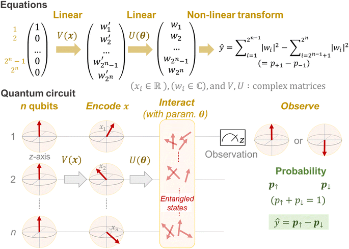
A mathematical expression of QCL for regression is not so complex (Fig. 1, see the Experimental section for derivation). The initial 2n-dimensional quantum state vector, expressed by (1, 0, …, 0)T, is transformed into another state w = (w1, w2, …, wn2)T by multiplying two complex operational matrices of V(x) and U(θ) (eqn (1)). Then, ŷ is calculated from the squares of w1, w2, …, wn2 (eqn (2)).
 | (1) |
 | (2) |
In a quantum circuit, V(x) and U(θ) correspond to the encoding and interaction steps of qubits, respectively (Fig. 1). Before calculation, all directions of qubit vectors are set upward along with the z-axis (corresponding to a vector of (1, 0, …, 0)T). The vectors are changed by the rotation gates of V(x). The encoded states are further rotated and interacted with according to another matrix U(θ). Finally, the direction of one qubit (or theoretically any number of qubits) is observed to obtain the interacted result.15,17 The regression model can learn a variety of functions because of the universality of the quantum circuit28 and the non-linear transformation steps during prediction (i.e., x ↦ V(x), θ ↦ U(θ) and the final prediction by eqn (2)).15
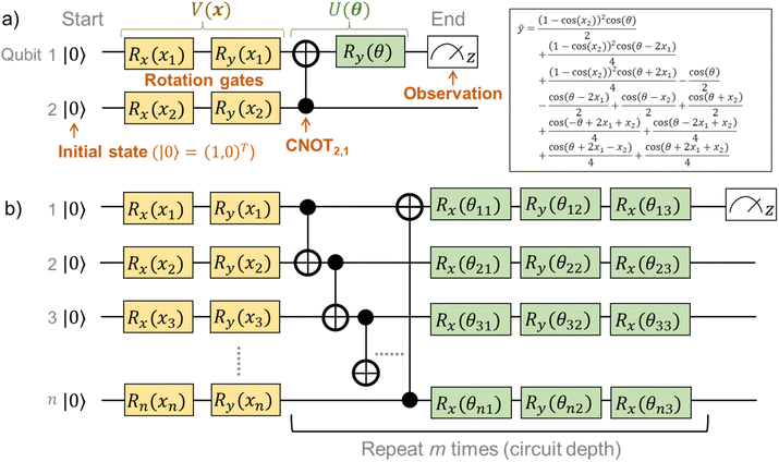
In eqn (1), the naïve determination of V and U is not easy because they are 2n × 2n-dimensional matrices (i.e., over 1018 parameters with n = 30). In QCL, the matrices are prepared by repeated products of elementary gate components, such as Ri,x(t), Ri,y(t), and CNOTi,j (eqn (3), Fig. 2).
 | (3) |
R i,x(t) and Ri,y(t) are rotation gates, changing the i-th qubit state and affecting nothing against the others.28 One qubit state (without entanglement) can be visualized as an arrow in a sphere (Bloch sphere, Fig. 2a). The gates change the angle of an i-th qubit along with the x- (or y-) axis (eqn (4), eqn (5)). A CNOTi,j gate can switch the state of the j-th qubit according to the condition of the i-th qubit (Fig. 2b, eqn (6)). The gate is similar to an XOR operation in classical circuits. The three components are known as universal gate sets, which can make an arbitrary quantum circuit from their products.28
 | (4) |
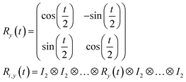 | (5) |
 | (6) |
Due to the restriction of quantum physics, the interacted state w itself is not observable by actual quantum systems. Instead, other parameters, such as the probabilities of upward (↑) or downward (↓) eigenstates, are experimentally observable (p↑ and p↓, respectively, Fig. 1). During actual quantum computing, such eigenstates are sampled via repeated calculations, and the probability difference between the two is calculated to obtain ŷ (eqn (7)).
 | (7) |
For clearer understanding, we calculated analytical solutions of ŷ with some simple quantum circuits (Table S1†). An example quantum circuit, encoding x = (x1,x2)T by four rotational gates, and interacting by one CNOT and one rotational gate, is shown in Fig. 3a. Even the simple circuit gives a very complex analytical solution of ŷ from eqn (2), consisting of repeated trigonometric functions (Fig. 3a). The complexity should mathematically correspond to the superparallel and entangled nature of the quantum system.
Regardless of the complex equation of ŷ in QCL, the value always ranges from −1 to +1 because of the unitary nature of the operational matrices, V and U (V†V = I, U†U = I, where † indicates complex conjugates).15,28 This study tries to clarify the actual effects of such complex yet systematic prediction algorithms for various regression tasks.
3 One-dimensional regression
We examined the basic regression properties of QCL models with simple one-dimensional functions of y = x, sin(x), and ex−1 (Fig. 4a). There are three major approaches to obtain ŷ: (a) calculate state vectors (eqn (1) and (2)) using classical computers, (b) sample frequencies of upward and downward eigenvalues to get their probabilities (p↑ and p↓, eqn (7)) using classical computers, and (c) conduct the sampling using real quantum computers. Currently, many studies obtain values by (a) or (b) due to the limited power of the quantum system.15,20–24 In the future, the role of (c) will be more critical with larger qubits because of the exponential calculation cost (in the order of 2n, eqn (1)). Here, predictions were mainly made by the most precise method of (a).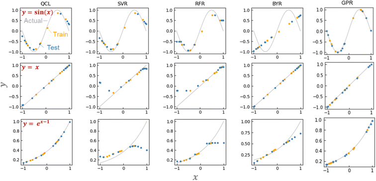 | ||
| Fig. 4 Predicting the function of y = sin(x), x, or, ex−1 using QCL, support vector machine for regression (SVR), random forest regression (RFR), Bayesian ridge regression (BYR), and Gaussian process regressor (GPR) (RBF + Dot-product). In the case of QCL, circuit parameters of n = 2 and m = 3 are chosen. Predictions were made from state-vector calculations. Other results are shown in Fig. S2.† (b) Predicting the function of y = sin(x) using an actual quantum computer (IBM Quantum) with m = 2, 3, or 4. Models were trained by state-vector calculations. Full results are shown in Fig. S12.† | ||
Preliminary optimization of quantum circuits15,17 and our optimization revealed that the following configuration was concise and practical for regression tasks (for details, see results and explanations in Fig. S1†). First, the inputted value x should be encoded by two rotational gates Ri,y(xi) and Ri,x(xi). Then, neighboring qubits had to be made to interact with CNOT gates, with θ-dependent gate rotation Ri,y(θj)Ri,x(θj+1)Ri,y(θj+2). The CNOT interaction and rotation should be repeated m times (Fig. 3b and S1†).
Some 1notes on circuit design should be mentioned. Mitarai et al. proposed15 the use of sin−1 or cos−1 to preconvert xi for linear encoding of the inputted value (Table S1†). On the other hand, we noticed that the conversion induced unfavorable bending of ŷ around |xi| ≅ 1, giving prediction errors (Fig. S1†). The bending was caused by the large curvature of the inverse functions (sin−1, cos−1) near ±1.
For qubit interaction, three gates, such as Ry, Rx, and Ry, were introduced for one qubit. The selection was because at least three gates are needed for arbitrary rotation for the complex vectors (i.e., X–Y decomposition).15 Instead of using systematic CNOT gates,17 non-parameterized random qubit interactions, known as the Transverse-field Ising model, could be employed.15 However, the regression was unstable and sometimes failed, depending on the randomness of the qubit interactions with a small circuit depth m ≤ 3, which motivated us to use repeated CNOT gates (Fig. S1†).
A QCL circuit with the qubit number of n = 2 and the depth of m = 3 was selected to learn the one-dimensional functions. Here, practically a one-dimensional vector x = (x1,x1) was encoded in the two-qubit circuit, enabling the higher expressiveness of fθ(x) (Fig. S1†). The final output was scaled by a constant prefactor of two as a hyperparameter unless noted otherwise (ŷ ↦ 2ŷ).15,17
QCL circuit was able to learn versatile functions of y = x, sin(x/2), sin(x), and ex−1 (Fig. 4a and S2†). The machine learning model was trained with about six training datasets randomly sampled, and they predicted about ten random testing data. No significant prediction errors were detected (Fig. 4a and S2†).
The unique advantage of the QCL model is highlighted by comparing it with the conventional regression models.18 We examined standard algorithms of support vector machine for regression (SVR), random forest regression (RFR), Bayesian ridge regression (BYR), and Gaussian process regressor (GPR) (Fig. 4a, S2, S3 and Table S2†).5 SVR works on the kernel trick, enabling the learning of even non-linear functions. RFR is a standard ensemble model of decision trees. Its reliable prediction is frequently employed with experimental material databases.5 BYR is a robust model for probabilistic linear regression, potentially strong against small datasets. GPR is similar to SVR, but its stochastic process can offer more flexible fitting with smaller datasets.
SVR, RFR, and BYR could not predict either y = x, sin(x), or ex−1. Prediction in extrapolating regions, where xi and ŷ range out of the training datasets, was unsuccessful (Fig. 4a and S2†). The SVR model assuming a non-linear Gaussian kernel mimicked sin(x), but gave a bent curve in the untrained regions of y = x. RFR displayed similar responses to SVR, with the unfavorable step-wise prediction by the noncontinuous decision-tree algorithm. The linear BYR model was predictable of y = x, but never of sin(x). Even though their hyperparameters were changed, the three models could not predict the functions (Fig. S3†). Due to the algorithm biases, many conventional supervised models could not switch linear and non-linear predictions.
We also examined more complex machine learning models, GPR and multilayer perceptron (MLP). GPR with radial basis function (RBF)-type kernels offered promising predictions due to their non-linear and stochastic algorithms (Fig. 4a, S3†).18 MLPs with different activation functions (ReLu, tanh, and sigmoid) and hidden layer numbers (1 to 4) did not afford sufficient performances. The models could switch linear and non-linear functions, but larger errors were obtained because of too many trainable parameters against the inputted data.
The performances of the regression models were validated by repeating the random data preparation and learning processes 30 times (Fig. S4, Table S3†). On average, two GPR models with RBF or RBF + Dot-product kernels exhibited the smallest error. The following best was the QCL regression: the model, capable of handling linear and non-linear interactions from small databases, offers a new option for solving regression tasks of various datasets.
4 Analyzing the regression steps of QCL
Although QCL models work on complex prediction algorithms (e.g., Table S1†), their estimation steps can be visualized (Fig. S5†). As defined in eqn (1), a quantum state is expressed by a complex vector of w = (w1, …, wn2)T (wi ∈![[Doublestruck C]](https://www.rsc.org/images/entities/char_e166.gif) ). We showed the change of coordinates wi in a simple example circuit of U(θ)V(x) = R1,y(θ)·CNOT1,2·R2,x(x)·R1,x(x) (θ = 1.0, x = 0.6) for a two-qubit system (Fig. S5a†). The applications of R1,x and R2,x gates changed w1 to w4 by shifting the complex coordinates of w2, w3, and w4. Then, w2 and w4 were swapped by the CNOT2,1 gate. The final output of ŷ = |w1|2 + |w2|2 − |w3|2 − |w4|2 (eqn (2)) was given followed by the rotation with R1,y. Although state vectors are not observable in the real world, state-vector simulation reveals such rotation and swapping effects by quantum gates. Developing more sophisticated visualization methods (e.g., heatmap for neural networks)11 is needed to provide deeper insights into more explainable QCL.
). We showed the change of coordinates wi in a simple example circuit of U(θ)V(x) = R1,y(θ)·CNOT1,2·R2,x(x)·R1,x(x) (θ = 1.0, x = 0.6) for a two-qubit system (Fig. S5a†). The applications of R1,x and R2,x gates changed w1 to w4 by shifting the complex coordinates of w2, w3, and w4. Then, w2 and w4 were swapped by the CNOT2,1 gate. The final output of ŷ = |w1|2 + |w2|2 − |w3|2 − |w4|2 (eqn (2)) was given followed by the rotation with R1,y. Although state vectors are not observable in the real world, state-vector simulation reveals such rotation and swapping effects by quantum gates. Developing more sophisticated visualization methods (e.g., heatmap for neural networks)11 is needed to provide deeper insights into more explainable QCL.
We calculated |wi|2 for the trained QCL models of y = sin(x) and x (Fig. 5a, b and S6†). Bending curves were observed for each term against x even with the linear function of y = x. This means that the QCL model worked through non-linear processes even with linear systems. The final output was made from the slight difference of |w1|2 + |w2|2 and |w3|2 + |w4|2.
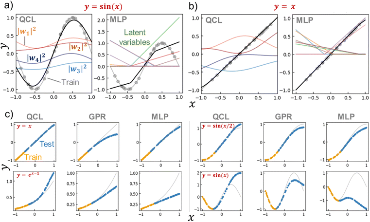 | ||
| Fig. 5 (a) Prediction process of y = sin(x) by a trained QCL model (m = 3, n = 2) or multilayer perceptron (MLP, 8-dimensional hidden layer and activation function of ReLu). The model was trained with 24 random records (gray plots). Black lines show predictions, and colored lines represent latent variables. (b) Prediction process for y = x. (c) Extrapolating predictions by QCL, GPR (RBF), and MLP models. After randomly generating 100 points, 70% of the data with high y were selected as testing (extrapolating) data. Full results are shown in Fig. S7 and S8.† | ||
As a control for QCL, MLP regressors were examined for prediction. The MLP model contained one 8- (or 16-) dimensional hidden layer for prediction with the standard non-linear activation function of ReLu or tanh.29 The overall design of QCL and MLP is slightly similar (Fig. S5b†). Both models encode x to the first latent vector w′, convert into another state of w by a θ-dependent transformation, and finally calculate ŷ from w. The main differences are (a) QCL maintains complex latent variables, whereas MLP usually has real numbers, and (b) only linear (or more precisely, unitary) transformation is available by QCL during the conversion of w′ to w.
MLP models were not predictive of the one-dimensional functions with small training data (around 20 records, Fig. 5a, S6†). A simple formula of y = sin(x) could not be fitted by MLP, even though different hyperparameters were employed (hidden layer sizes of 8 or 16 and activation functions of ReLu or tanh, Fig. S6†). The simplest y = x was successful, yet y = sin(x/2) and ex−1 were partially failing. Although complexing the circuit design, deep learning, will enhance fitting results, it also induces overfitting problems and requires larger datasets.
5 Keys to extrapolation by QCL
QCL affords promising prediction performances in extrapolating regions. We try to shed light on the reason by clarifying the requirements for extrapolation. First, the regression algorithms must provide ŷ outside the scope of trained y. Several models, such as decision trees and SVRs with RBF kernels, would not meet the criterion (Fig. 4). Second, the algorithms have to mimic the original data trend. For a simple example case, a quadratic function can perfectly predict the responses of ideal free falling. On the other hand, nobody knows most systems' exact functions and explanatory parameters. Instead, researchers should provide appropriate algorithms and parameters from their domain knowledge to come close to the ground truth.The QCL model is specialized in mimicking the gently sloping, non-linear functions. The model gave better performances in predicting linear, ex−1, and sin(x/2) functions compared to GPR and MLP (Fig. 5, S7 and S8†). The prediction error did not change drastically even though the extrapolation ratio in the dataset was changed from 10% to 90%, whereas others did (Fig. S8†). On the other hand, poorer results were obtained with steeper functions, sin(x) and sin(2x). The QCL model with the current parameter was unable to fit sin(2x) (n = 2, m = 3, Fig. S 2†). The results indicated that the current QCL model was specialized in predicting gently sloping, non-linear functions.
Of course, QCL models can be tuned to fit sin(2x) by optimizing hyperparameters (e.g., change the scaling prefactor c for prediction of ŷ ↦ cŷ, Fig. S9†). With a larger prefactor, more accurate fitting was achieved by QCL. However, the steeper fitting simultaneously spoiled the extrapolating prediction, yielding larger errors; the tuning to complex curves induced a side effect against extrapolation tasks. In this article, we decided to focus on the gently sloping, non-linear aspect of QCL with the specific configuration mentioned before. The character was also beneficial in predicting molecular properties from chemical structures (vide infra).
The smooth characteristics of the QCL model originated from the small trainable parameters and the regularization effect of quantum gates. The model had much smaller trainable parameters than MLP. The dimension of θ for QCL (n = 2, m = 3) was only 15, whereas 27 and 51 parameters were needed even for the unsuccessful MLP models (with hidden layer dimensions of 8 and 16, respectively). The smaller trainable parameters and continuous sinusoidal basis resulted in smooth curves. Furthermore, the unitary restriction of |w1|2 + |w2|2 + |w3|2 + |w4|2 = 1 should also have suppressed the outlier prediction as the regularization.
The smooth regression design was beneficial to fitting functions with noises (Fig. S10†). QCL, GPR, and MLP models were fitted with sin(x) or x with Gaussian random noises. QCL and GPR could basically fit the data when the noise level was 0 to ca. 40% to the original functions. On the other hand, the predictions by standard MLP were easily bent unnaturally because of the overfitting of the noised data. The smaller trainable parameters and unitary restriction of QCL should have contributed to adequate noise tolerance.
In summary, the current QCL model has a chance to outperform conventional linear and non-linear regression algorithms when smooth curves are supposed with the original datasets. Although the actual chemical and material systems do not always meet the requirement, the success in sparse (linear) modeling5,11 encourages researchers to expand the idea to smooth non-linear functions by QCL or other algorithms. Further tuning of QCL models will also offer capabilities of more complex functions, which should be examined in future research.
6 Prediction by an actual quantum computer
The biggest problem of QCL is the long calculation time with large qubit systems. The training time increased exponentially against the number of qubits n, and became significant (1 to 102 seconds) around n = 8 even with one-dimensional datasets (Fig. S 11†).Instead of calculating state vectors using eqn (1), prediction can also be made by observing the actual quantum system's eigenvalues: this is the real QCL (eqn (7)). Calculation cost will not increase exponentially because nature automatically does the calculation according to quantum mechanics.
The probabilistic sampling was examined with an IBM quantum computing machine (Fig. S 12†). The model was trained via the state-vector method. Then, we calculated statistical probabilities of upward (↑) or downward (↓) eigenvalues (p↑ or p↓) from the quantum system to predict ŷ = p↑ − p↓ (eqn (7)).
Quantum sampling suffered from more significant prediction errors than the classical state-vector calculation. The mean squared error (MSE) for the training dataset of y = sin(x), with a circuit of qubit number n = 2 and depth m = 2, was 0.0007 and 0.15 for state-vector and quantum sampling methods, respectively. When the circuit depth was increased to 3 or 4, the predicted values did not look like the original trigonometric curves. The errors were mainly caused by the computational noise of the quantum system (Fig. S12†).19 For practical usage, the number of quantum gates in the circuit must be reduced to suppress the effects of noise. More facile access to quantum machines is also essential because calculation takes about 101–103 seconds to predict just one record by the heavily crowded cloud system. The superparallel advantage of quantum machines for QCL will be achieved when the computers can handle large qubit numbers n (≫ 10) with negligible noise and prompt server responses.
Apart from hardware, the development of theoretical approaches is also essential. For instance, QCL accepts the limited domain of ŷ and xi. The unitarity of operational matrices restricts the predicted value of −1 ≤ ŷ ≤ 1. Although not mandatory, the explanatory variable xi should range in −π ≤ xi ≤ π owing to the periodicity of trigonometric functions in rotational gates (eqn (4) and (5)). For practical regression tasks, linear or non-linear conversion may be needed, whereas xi and y were set in [−1,+1] in this theoretical study (e.g., use of sigmoid: 1/(1 + e−x) and logit: log(ŷ/(1 − ŷ))).
7 Predicting molecular properties
We examined the QCL models to predict experimental molecular properties from their structures. Four standard experimental databases of (a) log solubility in water (estimating the aqueous solubility: ESOL),9 (b) melting point (Jean-Claude Bradley open melting point dataset),30 (c) octanol/water distribution coefficient (lipophilicity: Lipo),9 and (d) hydration free energy of small molecules in water (Solv)9 were selected as the benchmark. Regardless of the qubit limitations, the benefit of QCL was observed with actual materials- or chemo-informatics tasks.As explanatory variables, molecular features in the databases were calculated by a conventional ca. 200-dimensional descriptor algorithm of RDKit.31 The method can facilely quantify molecular characteristics by various indicators, such as molecular weight and the number of specific atoms in a molecule. Due to the high calculation cost of QCL, the descriptors were compressed to an 8-dimensional vector by principal component analysis.32 All explanatory and target variables were normalized in [−1,+1].
Small datasets were prepared artificially, assuming the actual materials informatics projects. From the master databases, 8, 16, 32, 64, 128, 256, or 512 records were sampled randomly. Then, the top 20% records of y were extracted as the testing data: these were model tasks for extrapolating regression. The random selection and regression tasks were repeated 2000/(dataset size) times for statistical verification (Fig. S13†).
QCL improved the prediction performance more than conventional models with several conditions. For instance, QCL exhibited the smallest MSE of 0.25 for the testing data, with the melting point database of 64 random records (Fig. 6a). Larger errors were observed with other models (RFR: 0.35, SVR: 0.30, BYR: 0.57, GPR: 0.61). Most of the ŷ by RFR and SVR ranged in the region of only trained y, meaning that extrapolation was unsuccessful, due to their decision-tree and radical basis kernel-based algorithms.2
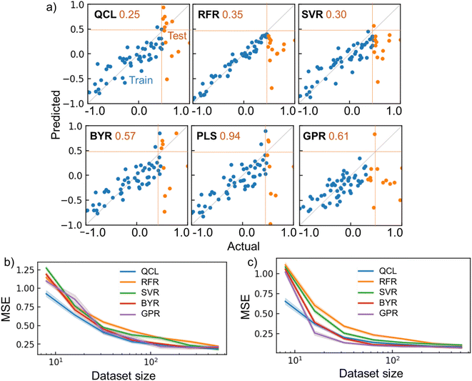 | ||
| Fig. 6 Regression results for chemical properties. (a) Actual and predicted parameters for the melting point dataset, using QCL (n = 8, m = 3) and other regressors. Dataset size was 64. The top 20% of y records were extracted as testing data, whose MSE is shown as orange numbers. (b) MSE for the regression tasks of melting point as a function of dataset size. Datasets were generated randomly and repeatedly. Transparent regions show standard errors with 68% confidence intervals. Results for PLS are not shown because the average MSE was too large. (c) Results for ESOL. The results with other databases (Fig. S14†) and results for interpolating tasks are shown in Fig. S15 and S16.† RBF + Dot-product was used for GPR. | ||
Linear-compatible models of BYR and GPR made some extrapolating predictions, exceeding the maximum y of training records (Fig. 6a). However, the model underestimated several test cases, giving large MSEs of 0.57 and 0.61, respectively. Another linear regression algorithm, partial least squares regression (PLS), was also examined as a regular model for materials informatics.33 Nevertheless, the model suffered from the largest MSE of 0.94. We doubt that the linear models could not faithfully catch up with the nonlinearity of the current experimental systems.
The models' performances were examined by repeating the random shuffling and regressions (Fig. 6b, c, S14†). Up to the dataset size of 100, QCL almost displayed the smallest error of the models (Fig. 6b). The quantum model was also robust against tiny datasets of ESOL and Solv (Fig. 6c and S14†). The QCL model also benefited from regular interpolating regression tasks, where 20% of testing data were sampled randomly (Fig. S15†). The model exhibited the best performance with the ESOL datasets, up to 32 records. Naturally, other models sometimes outperformed QCL under different conditions. There is no omnipotent algorithm applicable to any problem (no-free-lunch theorem).34 More careful analysis of predicting processes for each case is needed to pursue better performances in future research.
Although we currently have no clear clue about the remarkable performances of QCL, the gently sloping assumption of datasets might be a key to prediction. As demonstrated with the one-dimensional functions, the QCL model could fit linear and smooth curves (Fig. 4). If the experimental molecular structure (x)–property (y) relationships were not so fluctuated, their data trend could be mimicked by QCL. We are examining the data trends more carefully by considering the multivariable factors and distinguishing which functions are suitable for QCL.
A drawback of QCL for material exploration is the limited dimension of explanatory parameters. If conventional models conducted regressions without dimension reduction, they offered better performances than QCL (Fig. S14 and S15†). From another perspective, however, we can understand that the still large prediction errors by QCL were soluble by expanding the dimension. Preliminarily selecting essential parameters by other methods, such as sparse modeling,12 will also be critical to utilize QCL.
The encoding method of x to quantum circuits is also a challenge of QCL.15–17,26 The current model did not require two qubits for one variable of xi, in contrast to one-dimensional regressions (Fig. S1†). No significant improvement in prediction was detected even though the descriptors were compressed to 4-dimensional vectors and inputted to the 8-qubit model (i.e., x = (x1,x1, x2,x2, …, x4,x4), Fig. S16†). The success may be explained by the exponential nature of the state vectors (i.e., 2n-dimensional vectors and fully connected interactions). Encoding multiple values to one qubit is gradually becoming possible,26,28 whose circuit optimization will also increase the dimensions of explanatory parameters.
8 Conclusions
We examined the fundamental steps of quantum circuit learning (QCL) for regression and prediction performances of experimental molecular properties. The superparallel and entanglement nature of the quantum systems led to the exponential increase of the model complexity along with qubit numbers. Our study showed that the unitarity quantum operations contributed to the flexible fitting of linear and smooth non-linear functions, even from small datasets and extrapolating regions. QCL models had a chance to outperform conventional models with several experimental molecule databases. The long simulation time of QCL by classical computers is a challenge for practical applications. However, it is intrinsically soluble by developing algorithms and hardware. Supercomputers can now handle over 30 qubits,35,36 whose simulations will hint us at a more efficient way of calculations. We are also continuing to examine the potential of QCL with various material and chemical prediction tasks.9 Experimental section
9.1 Data and software availability
Programs and databases used in this study are available as open access via GitHub (https://github.com/KanHatakeyama/qcl).9.2 Deriving equations for a regression model of QCL
A regression model eqn (2) can be derived according to quantum mechanics and computing theory.28 A state of one qubit is typically expressed with a linear combination of two basis vectors, |0〉 and |1〉 (eqn (8)). | (8) |
For an n-qubit system, 2n-dimensional bases are needed to describe an arbitrary quantum state because of quantum entanglement.28 Their bases can be made by the tensor products of |0〉 and |1〉 (eqn (9)).
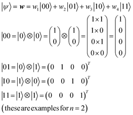 | (9) |
By quantum computing, the initial state of |0…0 = |0〉 ⊗ |0〉 ⊗…⊗|0〉 = (10…0)T is transformed into another form of |ψ〉 by repeated application of quantum gates (e.g., Rx, Ry, and CNOT), as unitary matrices (eqn (1) and (3)). In actual quantum systems, the state vector |ψ〉 itself cannot be observed, but expected values of some Hermitian operators are observable. Although there are many observation ways, the most straightforward and popular operation is to detect upward (↑) or downward (↓) eigenvectors for one qubit against the z-axis (eqn (7)).15,28 Its mathematical expression can be given by applying a Pauli's Z operator to the first qubit in a circuit (eqn (10)).
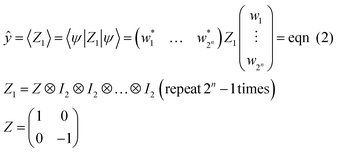 | (10) |
9.3 Calculation environment
Calculations were conducted with a Python 3 environment. Quantum computing libraries of Qulacs and Qiskit were introduced for simulation and actual quantum computing. Conventional regression models were made with scikit-learn.32 Analytical solutions were calculated with Sympy.37 Computations were done with a standard workstation without using graphics processing units (Intel Core i9-9900K CPU @ 3.60 GHz, 32 GB memory, and Ubuntu 16.04 operating system).9.4 Preparation of regression models
Unless noted otherwise, prediction models were generated with the configuration of Fig. 3b and state vector calculation using classical computers. The number of trainable parameters (or dimension of θ) were 3mn − 3m(n − 1). The latter term comes from the fact that rotation of the i-th (i > 1) qubit in the final depth layer does not affect the state of the 1st qubit for observation. Calculations were done using a Qulacs library.38 Final prediction was made using a constant factor of two as a hyperparameter (ŷ ↦ 2ŷ) except for Fig. S9.† Models were trained so that the summation of squared prediction errors (y − ŷ)2 for training data became smaller. A basin-hopping solver implemented in Scipy library39 was employed to optimize θ. Ising model Hamiltonian was also examined during circuit optimization instead of CNOT gates (Fig. S 1†). According to the method of Mitarai et al., Hamiltonian was made randomly, and its time evolution operator was generated via Suzuki–Trotter transformation (time step of 0.1).15For actual quantum computation and its simulation, predictions were conducted using a Qiskit library.40 For higher accuracy, the training parameter θ was preliminarily set by the state vector calculation by Qulacs. During prediction, sampling was repeated 1000 times for one record to obtain p↑ and p↓. The cloud service of IBM Quantum systems was used for quantum computing. Five-qubit systems were employed for sampling (mainly using a machine named ibmq_quito, having a quantum volume of 16 and clops of 2.5 K).
The following conventional models were introduced using the scikit-learn module: support vector machine for regression (SVR, radial basis function kernel), random forest regression (RFR, 100 decision trees), Bayesian ridge regression (BYR), Gaussian process regressor (GPR), partial least squares (PLS) regression (default dimension of 8). GPR models were constructed using some selected kernels plus a white kernel. Unless noted otherwise, default hyperparameters were used. MLP models were prepared using a Keras library.41 The model had a one-dimensional input layer, one (or multiple) 8- or 16-dimensional hidden layer(s), and a one-dimensional output layer (multiple hidden layers were examined in Fig. S3 and S4†). Relu, sigmoid, or tanh activation functions were introduced in the model. All training data (24 records) were simultaneously inputted into the model, using MSE loss and Adam optimizer. Due to the limited records, training was systematically repeated for 1000 epochs without making validation datasets.
9.5 Regression of one-dimensional functions
In Fig. 4 and related figures, regression models were examined with one-dimensional functions of y = x, sin(ax), ex−1(a:const.) with −1 ≤ x,y ≤ +1. Random N = 20 records were sampled to prepare a master dataset. For simplicity, no noise was added to the dataset. Then, the top 10%, lowest 10%, and other random 20% of the records were extracted as the testing data. The rest 60% was used for training. In Fig. S11,†N was set to be 50 for more accurate calculation time estimation. In Fig. S12,†N = 10 was used because of a long access time to connect the IBM cloud server. For extrapolation tasks, random N = 10 0 records were generated and 10, 30, 50, 70, or 90% of the data were used for testing (Fig. S14†). Gaussian random noise was added in Fig. S10.†9.6 Chemical property regression
Four types of standard experimental molecular databases were introduced: (a) log solubility in water (estimating the aqueous solubility: ESOL), (b) melting point (Jean-Claude Bradley open melting point dataset), (c) octanol/water distribution coefficient (lipophilicity: Lipo), and (d) hydration free energy of small molecules in water (Solv).9 Features of molecules were quantified as about 200-dimensional molecular descriptors by an RDKit library (Table S4†). Then, the descriptors were compressed to 8-dimensional vectors by principal component analysis by a scikit-learn module.32 In Fig. S16,† descriptors were compressed to 4-dimensional vectors instead.For regression, quantum circuit models with n = 8 and m = 3 were employed. Datasets were prepared by randomly sampling 8, 16, 32, 64, 128, 256, or 512 records from the master databases (Fig. S13†). All variables (y,xi) in each dataset were normalized in the range of [−1,+1]. As testing data, 20% of the top y records were extracted in Fig. 6 and S14.† Random 20% data were extracted for testing in Fig. S15 and S16.† The random dataset generation and prediction processes were repeated 2000/ (dataset size) times for statistical verification. The figures display the test data's mean squared error (MSE) as box plots. The maximum y-axis was set to be 4 for easier understanding (excessive outliers are not shown in the graphs). Unless noted otherwise, default hyperparameters of the scikit-learn library were used for the conventional models.
Data availability
Data and processing scripts for this paper, including databases and regression programs, are available at GitHub (https://github.com/KanHatakeyama/qcl).Author contributions
All authors have given approval to the final version of the manuscript.Conflicts of interest
The authors have no conflicts of interest to declare.Acknowledgements
This work was partially supported by Grants-in-Aid for Scientific Research (No. 21H04695, 18H05515, 20H05298, 22H04623, and 21H02017) from MEXT, Japan. The work was partially supported by JST FOREST Program (Grant Number JPMJFR213V, Japan), JST CREST (JPMJCR21O1), and the Research Institute for Science and Engineering, Waseda University.Notes and references
- S. Hong, C. H. Liow, J. M. Yuk, H. R. Byon, Y. Yang, E. Cho, J. Yeom, G. Park, H. Kang, S. Kim, Y. Shim, M. Na, C. Jeong, G. Hwang, H. Kim, H. Kim, S. Eom, S. Cho, H. Jun, Y. Lee, A. Baucour, K. Bang, M. Kim, S. Yun, J. Ryu, Y. Han, A. Jetybayeva, P. P. Choi, J. C. Agar, S. V. Kalinin, P. W. Voorhees, P. Littlewood and H. M. Lee, ACS Nano, 2021, 15, 3971–3995 CrossRef.
- J. Schmidt, M. R. G. Marques, S. Botti and M. A. L. Marques, npj Comput. Mater., 2019, 5, 83 CrossRef.
- M. Scheffler, M. Aeschlimann, M. Albrecht, T. Bereau, H. J. Bungartz, C. Felser, M. Greiner, A. Gross, C. T. Koch, K. Kremer, W. E. Nagel, M. Scheidgen, C. Woll and C. Draxl, Nature, 2022, 604, 635–642 CrossRef.
- Y. C. Lo, S. E. Rensi, W. Torng and R. B. Altman, Drug Discovery Today, 2018, 23, 1538–1546 CrossRef PubMed.
- R. Ramprasad, R. Batra, G. Pilania, A. Mannodi-Kanakkithodi and C. Kim, npj Comput. Mater., 2017, 3, 54 CrossRef.
- Y. LeCun, Y. Bengio and G. Hinton, Nature, 2015, 521, 436–444 CrossRef CAS PubMed.
- K. Hatakeyama-Sato and K. Oyaizu, Commun. Mater., 2020, 1, 49 CrossRef.
- K. Hatakeyama-Sato, T. Tezuka, M. Umeki and K. Oyaizu, J. Am. Chem. Soc., 2020, 142, 3301–3305 CrossRef CAS.
- Z. Wu, B. Ramsundar, E. N. Feinberg, J. Gomes, C. Geniesse, A. S. Pappu, K. Leswing and V. Pande, Chem. Sci., 2018, 9, 513–530 RSC.
- S. Nagasawa, E. Al-Naamani and A. Saeki, J. Phys. Chem. Lett., 2018, 9, 2639–2646 CrossRef PubMed.
- H. Yamada, C. Liu, S. Wu, Y. Koyama, S. Ju, J. Shiomi, J. Morikawa and R. Yoshida, ACS Cent. Sci., 2019, 5, 1717–1730 CrossRef PubMed.
- R. Mizuguchi, Y. Igarashi, H. Imai and Y. Oaki, Nanoscale, 2021, 13, 3853–3859 RSC.
- J. Mairal, F. Bach and J. Ponce, arXiv, 2014, preprint, arXiv:1411.3230 Search PubMed.
- H. Numazawa, Y. Igarashi, K. Sato, H. Imai and Y. Oaki, Adv. Theory Simul., 2019, 2, 1900130 CrossRef.
- K. Mitarai, M. Negoro, M. Kitagawa and K. Fujii, Phys. Rev. A, 2018, 98, 032309 CrossRef.
- J. G. Liu and L. Wang, Phys. Rev. A, 2018, 98, 062324 CrossRef CAS.
- T. Suzuki and M. Katouda, J. Phys. Commun., 2020, 4, 125012 CrossRef.
- T. Hastie, R. Tibshirani and J. Friedman, The Elements of Statistical Learning, Springer, New York, NY, 2009 Search PubMed.
- K. Bharti, A. Cervera-Lierta, T. H. Kyaw, T. Haug, S. Alperin-Lea, A. Anand, M. Degroote, H. Heimonen, J. S. Kottmann, T. Menke, W.-K. Mok, S. Sim, L.-C. Kwek and A. Aspuru-Guzik, Rev. Mod. Phys., 2022, 94, 015004 CrossRef CAS.
- J. Preskill, Quantum, 2018, 2, 79 CrossRef.
- Y. Cao, J. Romero, J. P. Olson, M. Degroote, P. D. Johnson, M. Kieferova, I. D. Kivlichan, T. Menke, B. Peropadre, N. P. D. Sawaya, S. Sim, L. Veis and A. Aspuru-Guzik, Chem. Rev., 2019, 119, 10856–10915 CrossRef CAS PubMed.
- I. G. Ryabinkin, T. C. Yen, S. N. Genin and A. F. Izmaylov, J. Chem. Theory Comput., 2018, 14, 6317–6326 CrossRef.
- R. Xia and S. Kais, Nat. Commun., 2018, 9, 4195 CrossRef PubMed.
- J. Biamonte, P. Wittek, N. Pancotti, P. Rebentrost, N. Wiebe and S. Lloyd, Nature, 2017, 549, 195–202 CrossRef.
- S. A. Stein, R. L'Abbate, W. Mu, Y. Liu, B. Baheri, Y. Mao, Q. Guan, A. Li and B. Fang, arXiv, 2021, preprint, arXiv:2012.00256 Search PubMed.
- M. Schuld, A. Bocharov, K. M. Svore and N. Wiebe, Phys. Rev. A, 2020, 101, 032308 CrossRef.
- Y. Takaki, K. Mitarai, M. Negoro, K. Fujii and M. Kitagawa, Phys. Rev. A, 2021, 103 Search PubMed.
- M. A. Nielsen and I. L. Chuang, Quantum Computation and Quantum Information: 10th Anniversary Edition, Cambridge University Press, Cambridge, 2010 Search PubMed.
- L. Alzubaidi, J. Zhang, A. J. Humaidi, A. Al-Dujaili, Y. Duan, O. Al-Shamma, J. Santamaria, M. A. Fadhel, M. Al-Amidie and L. Farhan, J. Big Data, 2021, 8, 53 CrossRef PubMed.
- J.-C. Bradley, Open Melting Point Dataset, 2014, DOI:10.6084/m9.figshare.1031637.
- RDKit: Open-source cheminformatics, http://www.rdkit.org Search PubMed.
- F. Pedregosa, G. Varoquaux, A. Gramfort, V. Michel, B. Thirion, O. Grisel, M. Blondel, P. Prettenhofer, R. Weiss, V. Dubourg, J. Vanderplas, A. Passos, D. Cournapeau, M. Brucher, M. Perrot and E. Duchesnay, J. Mach. Learn. Res., 2011, 12, 2825–2830 Search PubMed.
- K. Rajan, Mater. Today, 2005, 8, 38–45 CrossRef CAS.
- D. H. Wolpert and W. G. Macready, IEEE Trans. Evol. Comput., 1997, 1, 67–82 CrossRef.
- S. Imamura, M. Yamazaki, T. Honda, A. Kasagi, A. Tabuchi, H. Nakao, N. Fukumoto and K. Nakashima, arXiv, 2022, preprint, arXiv:2203.16044 Search PubMed.
- Z. Wang, Z. Chen, S. Wang, W. Li, Y. Gu, G. Guo and Z. Wei, Sci. Rep., 2021, 11, 355 CrossRef CAS.
- A. Meurer, C. P. Smith, M. Paprocki, O. Čertík, S. B. Kirpichev, M. Rocklin, A. Kumar, S. Ivanov, J. K. Moore, S. Singh, T. Rathnayake, S. Vig, B. E. Granger, R. P. Muller, F. Bonazzi, H. Gupta, S. Vats, F. Johansson, F. Pedregosa, M. J. Curry, A. R. Terrel, Š. Roučka, A. Saboo, I. Fernando, S. Kulal, R. Cimrman and A. Scopatz, PeerJ Comput. Sci., 2017, 3, e103 CrossRef.
- Y. Suzuki, Y. Kawase, Y. Masumura, Y. Hiraga, M. Nakadai, J. Chen, K. M. Nakanishi, K. Mitarai, R. Imai, S. Tamiya, T. Yamamoto, T. Yan, T. Kawakubo, Y. O. Nakagawa, Y. Ibe, Y. Zhang, H. Yamashita, H. Yoshimura, A. Hayashi and K. Fujii, Quantum, 2021, 5, 559 CrossRef.
- P. Virtanen, R. Gommers, T. E. Oliphant, M. Haberland, T. Reddy, D. Cournapeau, E. Burovski, P. Peterson, W. Weckesser, J. Bright, S. J. van der Walt, M. Brett, J. Wilson, K. J. Millman, N. Mayorov, A. R. J. Nelson, E. Jones, R. Kern, E. Larson, C. J. Carey, I. Polat, Y. Feng, E. W. Moore, J. VanderPlas, D. Laxalde, J. Perktold, R. Cimrman, I. Henriksen, E. A. Quintero, C. R. Harris, A. M. Archibald, A. H. Ribeiro, F. Pedregosa, P. van Mulbregt and C. SciPy, Nat. Methods, 2020, 17, 261–272 CrossRef CAS PubMed.
- Qiskit: An Open-source Framework for Quantum Computing, https://zenodo.org/record/6476573, DOI:10.5281/zenodo.2573505.
- F. Chollet, Keras, https://github.com/fchollet/keras Search PubMed.
Footnote |
| † Electronic supplementary information (ESI) available. See DOI: https://doi.org/10.1039/d2dd00090c |
| This journal is © The Royal Society of Chemistry 2023 |

