A scalable neural network architecture for self-supervised tomographic image reconstruction

Abstract

We present a lightweight and scalable artificial neural network architecture which is used to reconstruct a tomographic image from a given sinogram. A self-supervised learning approach is used where the network iteratively generates an image that is then converted into a sinogram using the Radon transform; this new sinogram is then compared with the sinogram from the experimental dataset using a combined mean absolute error and structural similarity index measure loss function to update the weights of the network accordingly. We demonstrate that the network is able to reconstruct images that are larger than 1024 × 1024. Furthermore, it is shown that the new network is able to reconstruct images of higher quality than conventional reconstruction algorithms, such as the filtered back projection and iterative algorithms (SART, SIRT, CGLS), when sinograms with angular undersampling are used. The network is tested with simulated data as well as experimental synchrotron X-ray micro-tomography and X-ray diffraction computed tomography data.

---

Introduction

Machine learning, in particular deep learning, has revolutionised fields as diverse as image recognition and text translation over the past decade, replacing pre-determined, ‘hand-crafted’ algorithms with flexible neural networks which learn to perform a task from training on existing examples. In recent years, the application of deep neural networks (DNNs) in the life and physical sciences has also attracted a lot of interest.^1–4 Tomographic image reconstruction has witnessed a number of high-profile breakthroughs where DNNs match or even exceed the performance of state-of-the-art physics-based approaches.^5,6 The majority of work applying DNNs for tomographic image reconstruction has focused on enhancing the quality of real space images, which have been generated from sinograms by traditional algorithms, such as the filtered back projection.^7–9 A number of notable exceptions do exist, where supervised learning, and generative models have been used to automatically map from sinogram to real space.^5,10–16 While these methods are very promising, bottlenecks still exist to their application to image reconstruction due to their scalability (i.e. their ability to handle large images), their network size (large networks can be computationally very expensive) and particularly for applications where absolute values (as opposed to normalised values) are important in the reconstructed image, such as in chemical tomography and in quantitative analysis of attenuation-based tomography data.

The improved performance of both X-ray sources and detectors in recent times has seen a number of studies obtain rapid time-resolved data (i.e. spectra, patterns) from multiple positions within a single sample or else from a sample ensemble via the performing of time-resolved imaging/tomography experiments.^17–19 These ‘chemical imaging’ techniques have reached a stage whereby they enable the study of functional materials and devices in four or more dimensions i.e. obtaining spatially resolved (1D/2D) spectra/patterns in 2D/3D from an evolving sample, such as a catalytic reactor, a fuel cell or a Li-ion battery, as a function of time (1D) or imposed operating condition/state (e.g. temperature, pressure, potential, chemical environment).^20–26 The quantity and speed of this data acquisition poses challenges to traditional image reconstruction and analysis techniques. The limits to what is currently achievable with chemical imaging techniques is currently often determined by the density of sampling required for the sinogram in order to achieve good quality image reconstructions. Algorithms for improved reconstruction with more sparsely sampled sinograms are needed to unlock new levels of spatial and temporal resolution in chemical imaging.

The majority of popular existing algorithms for tomographic image reconstruction can be divided into two classes; direct methods and iterative methods. Direct methods such as filtered back projection (FBP) provide quick results which are artefact-free if there is an abundance of projections and data with high signal-to-noise ratio; iterative methods such as total-variation minimisation work well in sparse projection scenarios and/or data with low signal-to-noise ratio, but rely on prior knowledge and fine hyperparameter tuning.²⁷ Recently DNNs have emerged as a powerful new tool for image reconstruction. DNNs have been applied to learn the filters for FBP or map the FBP to a DNN,^28–31 to improve the quality of input projections/sinograms^32–35 or of output images from direct reconstruction techniques.^7,36–38

In 2018 the AUTOMAP network demonstrated the application of direct reconstructions of images from projections,⁵ however the size of image for which AUTOMAP can be applied is limited by the presence of densely connected layers with many parameters, which scale poorly with the number of pixels in the input. Alternative methods based on convolutional neural networks (CNNs) and generative adversarial networks (GANs) that include physical information have recently been proposed which show great promise for image reconstruction, with fewer restrictions of the sizes of data that can be treated.^39–42 The GAN approach has been demonstrated to be very useful for image reconstruction, but previous procedures rely on normalising sinogram and image values.³⁹ This is not necessarily a problem when the data analysis focuses on image segmentation, but in the case of chemical tomography where we are reconstructing images containing spectra at each pixel this information is essential;^43,44 the absolute values are also required when quantitative analysis of attenuation-based tomography data is performed (e.g. micro-CT).

In this work we introduce the SingleDigit2Image (SD2I) network – a simple, scalable generative network that can be used for direct conversion of sinogram to image (Fig. 1). The input of the SD2I is a random constant which preferably has a similar order of magnitude as the reconstructed image's signal. The SD2I acts as a generator network that creates an image based on the single number input; the generated image is then converted into a sinogram by the differentiable forward operator which is the Radon transform. This new sinogram is compared with the sinogram from the experimental dataset using a loss function and the weights of the SD2I network are updated accordingly. Our approach relies on a relatively simple and scalable architecture. We show that our approach can reconstruct a series of different modality tomography images with at least as good an accuracy as the FBP algorithm. We demonstrate the scalability of our method compared to the state-of-the-art methods. We also show that our method is able to deal with a commonly encountered challenge to FBP reconstruction, specifically sinograms exhibiting angular undersampling. We have tested our approach on a Shepp–Logan phantom as well as on experimental X-ray diffraction computed tomography (XRD-CT) and micro-CT sinogram data highlighting the flexibility and applicability of the method.

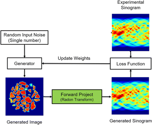Fig. 1 The flowchart of the SD2I training algorithm. The input of the SD2I is a random constant which preferably has a similar order of magnitude as the reconstructed image's signal. The generator generates an image based on the single input; the generated image is then converted into a sinogram by the forward operator, which is compared with the sinogram from the experimental dataset. The weights of the generator are updated by minimising the joint loss function with mean absolute error (MAE) and structural similarity index measure (SSIM).⁴⁵

SD2I architecture

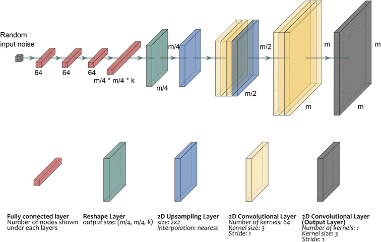
The architecture of the artificial neural network used for reconstructing the images from the sinograms is depicted in Fig. 2. There are two novelties in this design compared to other architectures previously proposed for tomographic image reconstruction. First, the SD2I network, as the name suggests, starts from a single number rather than a 2D image which significantly reduces the number of parameters in the architecture. In other networks, the input is a 2D image which is either flattened and connected to a dense layer containing 100s of neurons (e.g. 256 in the GANrec) or is followed by a series of 2D convolutional and downsampling layers with the final layer being flattened and connected to the aforementioned dense layer. The second novelty is related to the large dense layer and the convolutional layers that are connected to it which dramatically reduces the number of parameters in the network's architecture. In this paper, we are going to use two types of SD2I architectures which are called the SD2I and the SD2I with upsampling layers (SD2Iu) respectively. The SD2I presented in Fig. S1† shows an architecture that receives a single number as input and has a large fully connected layer in the middle. As this architecture lacks the encoder network present in both GANrec and AUTOMAP architectures, SD2I can allocate more parameters to augment the decoding network's size. Consequently, under the same model size constraints, SD2I is capable of reconstructing images with higher quality than GANrec and AUTOMAP. The impact of k factors on the performance of the SD2I network is also presented in Fig. S2 and Table S1.† Simultaneously, the SD2Iu architecture depicted in Fig. 2 possesses fewer parameters than the SD2I architecture, achieved by reducing the size of the fully connected layers. The network initially predicts an image at a lower resolution and subsequently upscales it to the original image size through the use of upsampling and convolutional layers. To clarify, the initial single number (input layer) is followed by three small dense layers, each containing 64 neurons. The third small dense layer is then connected to a larger dense layer consisting of (m/4) × (m/4) × k neurons, where m is the number of pixels in one dimension of the fully reconstructed images which have size equal to m × m. The k factor is an integer and increasing it can lead to better performance of the neural network but also increases the number of parameters. In this work and after initial testing, we used a range of k between 4 and 8; this range provides a good balance between network size/training speed and quality of reconstructed images (Fig. S3†). The large dense layer is then reshaped to a 2D layer of size, followed by an upsampling layer resulting in an image with size of (m/2, m/2). This is followed by three 2D convolutional layers and a second upsampling layer resulting in an image with size of (m, m). Each of these 2D convolutional layers has 64 filters with a kernel size of 3 and stride equal to 1. The final layer of the architecture is a 2D convolutional layer with one kernel (kernel size of 3) and stride equal to 1. We employed ReLU as the activation function for all hidden layers, except the final output layer. To determine the most suitable activation function for the output layer, we assessed the performance of various alternatives and ultimately selected the absolute function as our choice for the output layer.^46,47 The performance comparison of the various activation functions is illustrated in Fig. S4 and Table S2.† Our findings indicate that the absolute function outperforms the rest. Although ReLU could be considered as a potential alternative, we experienced numerous dead-pixel issues when using it, particularly with experimental data containing noise so for all results presented in this work we used the absolute function.

Fig. 2 A representation of the CNN reconstruction SD2I architecture with upsampling (SD2Iu). The kernel types and parameter settings are shown in the figure. The final fully connected layer size is adjusted by an integer k, which adjusts the number of kernels used as the input of the following reshape, upsampling and convolutional layers. All layers in the neural network use ReLU as their activation function, except for the final layer which employs the absolute value function.

Overall, the network starts with a single number (input layer) and yields a 2D image with size of (m, m) which is equal to the image size obtained with the conventional tomographic reconstruction algorithms. The SD2Iu's architecture allows for radical decrease in the number of parameters and allows it to reconstruct images that are more than 1028 × 1028 large.

While several deep learning approaches have proved very successful for CT reconstruction, a major barrier to their widespread adoption is that the number of parameters (and hence required computational resources) scales poorly as the size of sinogram increases. The new architecture that we propose, has at least an order of magnitude fewer parameters than existing deep learning approaches (e.g. Automap and GANrec), as shown in Fig. 3 and Table S3.† Note that for these tests it was not possible to use Automap on images larger than 128 × 128 pixels, due to memory constraints.

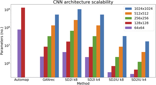Fig. 3 Comparison of the Automap, GANrec and SD2I architectures (U: upsampling) for reconstructing images of different sizes.

Results & discussion

Simulated data

We start by comparing the performance of our new architecture against the filtered back projection (FBP) algorithm and other neural network based reconstruction algorithms. For this comparison we use a sinogram created using the Shepp–Logan phantom with image size of 256 × 256 pixels; the sinogram size is 256 × 400 pixels, corresponding to detector elements and number of projections respectively. The reconstructed images are presented in Fig. 4 while Table 1 compares the results from the various reconstruction methods applied, using several common image quality metrics and specifically the mean absolute error (MAE), mean squared error (MSE), structural similarity index measure (SSIM)⁴⁵ and peak signal to noise ratio (PSNR). We find that all variants of our SD2I architecture outperform both GANrec and FBP across all metrics. The SD2I architectures that perform best are those where the convolutional part of the network is a single size, rather than including upsampling layers. However, even the SD2I architecture with upsampling convolutional layers (SD2Iu) (which has significantly fewer parameters than that without upsampling) performs very well. We also find that changing the size of the final dense layer in the SD2I architecture (the factor k) has a small but appreciable effect on the image quality. Somewhat surprisingly, of the architectures with no upsampling layers (SD2I), the one with the smaller final dense layer performs slightly better, this could be due to local minima trapping in the larger network. Nonetheless, the main point is that SD2I performs very well on the standard Shepp–Logan phantom, regardless of architecture hyperparameters (within a reasonable range). Adam was used as the optimisation algorithm,⁴⁸ a combined MAE and SSIM loss function⁴⁹ was used with the following formula:

Loss = (1 − μ) × MAE + μ × SSIM

here we used μ = 0.84 for all simulated Shepp–Logan images. The learning rate was set to 0.0005 for networks presented in this work. The learning rate was automatically reduced during training if the loss function was not decreasing after 300 iterations using a downscaling factor of 0.5 (Tensorflow ReduceLROnPlateau implementation⁵⁰); 6000 epochs were used during the image reconstruction process. It is important to note here that the various metrics provide only an indication of the image quality reconstruction and one should always inspect the resulting images regardless of the values of the various metrics. Reconstruction times are presented in Tables S4–S6.†

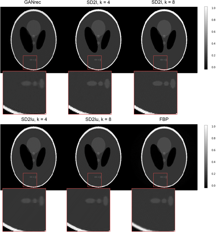Fig. 4 Comparison between the SD2I result and conventional reconstruction methods. The image size is 256 × 256, and reconstructed from the 256 × 400 Shepp–Logan sinogram.

Table 1 Accuracy. Comparison of approaches for a 256 × 400 Shepp–Logan sinogram. Metrics calculated using four significant figures for SSIM and PSNR and three significant figures for MAE and MSE

	GANrec	SD2I (k = 4)	SD2I (k = 8)	SD2Iu (k = 4)	SD2Iu (k = 8)	FBP
MAE	0.009714	0.0009582	0.0005762	0.001747	0.002600	0.007819
MSE	0.0006505	4.267 × 10^6	2.854 × 10 ^6	3.493 × 10^5	5.827 × 10^5	7.783 × 10^4
SSIM	0.9318	0.9988	0.99965	0.9974	0.9950	0.9565
PSNR	31.87	53.70	55.44	44.57	42.35	31.09

---

To demonstrate the enhancement in the quality of the reconstructed image as a result of the single digit input, we assessed the performance of the networks, specifically the SD2I and SD2Iu models, starting from the last fully connected layer. When the networks were provided with a 64-unit vector of ones (the same size as the fully connected layer preceding the final layer), the results were markedly poorer and could not compete with the SD2Iu in terms of reconstructing the 256 × 64 size sinogram. The results are presented in Fig. S5.†

Furthermore, we evaluated a pixel learning network that receives a single digit as input and consists of a singular extensive fully connected layer, equivalent to the total number of pixels in the image. This network, devoid of convolutional layers, equates to the iterative approach that learns each distinct pixel from a map of ones, utilizing the same training loop as SD2I. The results are compared with those from the SD2I, using a full range 256 × 400 sinogram, in Fig. S6.† It is evident that the presence of multiple fully connected layers and convolutional layers significantly assists the SD2I in producing far more precise and refined results compared to the straightforward pixel learning network.

Angular undersampling

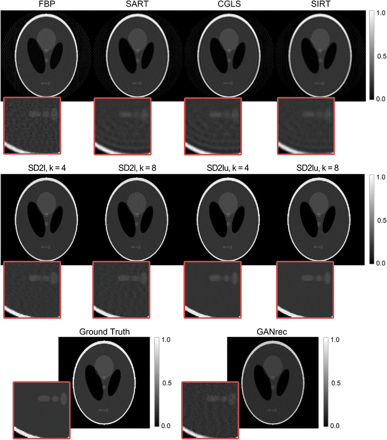
A striking advantage of many deep learning based reconstruction approaches, when compared to traditional methods, such as FBP, is their ability to achieve high quality reconstructions when only challenging data are practically available. These can be sinograms with angular undersampling, low signal-to-noise ratio or incomplete sinograms (e.g. not covering the full 0–180° angular range).^9,39 However, most of the approaches are applied on the FBP reconstructed images (i.e. post-processing of the reconstructed images) rather than performing directly the tomographic reconstruction and importantly rely on supervised learning which assumes (a) that artefact-free images (labelled data) are available and (b) that the networks can generalise (e.g. train with non-scientific datasets typically used for developing neural networks and yield high quality images when applied to experimental data). Unfortunately, these assumptions are rarely valid and the applicability of such networks to real experimental data is limited at best. Here, we show that the SD2I, apart from its ability to reconstruct large tomographic images in a self-supervised manner, is able to suppress the angular undersampling artefacts while performing the tomographic reconstruction. In Fig. 5, we show the reconstruction of the Shepp–Logan phantom with a severe angular-undersampling where we only have less than ¼ of the original sinogram projections (projections corresponding to ¼ of the detector elements). For comparison, also shown are the results obtained from the most often used iterative algorithms (SART, CGLS and SIRT) using the ASTRA Toolbox⁵¹ as well as from GANrec. Compared to all conventional reconstruction algorithms tested SD2I produces results with significantly fewer artefacts and much closer to the ground truth reconstruction. Importantly, it is clearly shown that the SD2Iu networks, which correspond to the smallest possible networks in terms of number of parameters, yield the best results. The use of the upsampling convolution layers actually improves the quality of the reconstruction, performing a function similar to denoising on the resultant images. It should be noted though that the network does not denoise the reconstructed images, it removes the angular undersampling artefacts. It therefore requires projection/sinogram data with high signal-to-noise ratio; it does not lead to higher quality reconstructed images than the FBP algorithm when the signal-to-noise ratio is low.

Fig. 5 Comparison between conventional and neural network reconstruction approaches with different parameter settings. The image size is 256 × 256, and reconstructed from the 256 × 64 Shepp–Logan sinogram.

Table 2 also shows the performance of the FBP, SIRT, CGLS, SART, GANrec and various SD2I architectures on undersampled Shepp–Logan Sinograms. These metrics confirm what is shown in the figures, with the SD2I outperforming other methods and the SD2I architecture with convolutional upsampling performing the best. The results in Fig. S7† show that this approach can be applied to larger image reconstruction tasks and the performance gains remain for SD2I. For calculating the SSIM and PSNR, we used the maximum possible pixel value as 1. A larger Shepp–Logan phantom image (512 × 512) was also tested (sinogram with size equal to 512 × 128) and the SD2I results are presented in Fig. S7 and Table S7.† The impact of the loss function is shown in Table S8.†

Table 2 Accuracy. Comparison of approaches for a 256 × 64 Shepp–Logan sinogram. 250 iterations were used for the SART, SIRT and CGLS algorithms. Metrics calculated using four significant figures

	MAE	MSE	SSIM	PSNR
FBP	0.01906	0.001405	0.6129	28.52
SART	0.01702	0.001851	0.7572	27.33
CGLS	0.01722	0.001717	0.7329	27.65
SIRT	0.01768	0.002327	0.7984	26.33
GANrec	0.02408	0.002521	0.7070	25.98
SD2I (k = 4)	0.004527	0.0001181	0.9776	39.27
SD2I (k = 8)	0.004548	0.0001269	0.9778	38.96
SD2Iu (k = 4)	0.003229	0.0001088	0.9911	39.29
SD2Iu (k = 8)	0.002881	0.00009763	0.9931	40.10

---

It should be noted here that the results for the various metrics strongly depend on the choice of the ground truth image. This is not an issue for the Shepp–Logan phantom but it is a problem for the experimental data where there is no ground truth image available. This means that the quality of the reconstructed images has to be done primarily through visual inspection as the results from the various metrics can be misleading. To illustrate this problem, we measured the performance of SD2I as well as FBP, SART, SIRT and CGLS using different images as the ground truth image for the Shepp–Logan image (Fig. S8 and Tables S9–S11†). If the FBP reconstructed image using the full projection set (400 projections) is used as the ground truth, then the metrics suggest that SIRT and CGLS outperform the SD2I. However, this is clearly not the case as shown in Fig. 5 and S7† and from the fact that the clean (real ground truth) Shepp–Logan phantom image shows worse results for all metrics (Table S10†). The result obtained with the CGLS method using the full projection set (400 projections) looks closer to the ground truth image compared to the FBP, SART and SIRT results obtained using the full projection set and for this reason it is used as the ground truth for evaluating the performance of the SD2I network for the experimental data. Finally, it is important to note that when the clean Shepp–Logan image (real ground truth) or the CGLS image obtained using the full projection set are used as the ground truth, it can be seen that the SD2I with less than ¼ projections (64 projections) outperforms FBP, SART and SIRT reconstructions using the full projection set (400 projections). This result further illustrates the accuracy of the SD2I reconstructions and the potential of this new network for data exhibiting angular undersampling.

Experimental data

We now turn our attention to testing the SD2I architecture on real experimental synchrotron X-ray tomography data. We obtain a ‘ground truth’ reconstruction in this case by reconstructing the images using CGLS with the full projection set. We then decrease the projection set to ¼ of the original size and compare the results of the reconstruction using CGLS, FBP, SART, SIRT and SD2I on the decreased sinogram.

First, we compare the results obtained from SD2Iu and the other methods using an experimental XRD-CT dataset acquired from a 3D printed SrNbO2N photocatalyst used for degradation of organic pollutants in water.⁵² The original sinograms of this dataset had 300 projections and 331 translation steps (the image size is then 331 × 331). The image reconstructed by CGLS with the full 300 projections is considered as the ground truth image when calculating the metrics shown in Table 3 while the reconstructed images using the various methods are presented in Fig. 6. The hyperparameters for the SD2I networks used in this work for the XRD-CT data were kept the same for all datasets and no tweaking was required (initial learning rate of 0.0005 with a decaying rate and a safe margin of 6000 epochs). It can be clearly seen that both the visual inspection and the metrics shown in Table 3 indicate that the SD2I performed the best among all the conventional methods we tested. The magnified region in Fig. 6 also shows that SD2I is able to retain very fine features present in the images, in this case corresponding to the channels and network of the 3D printed catalyst.

Table 3 Accuracy. Comparison of approaches for the example photocatalyst experimental XRD-CT image shown in Fig. 6. The CGLS with 300 projections is considered as the ground truth. Metrics calculated using four significant figures

	FBP	SART	CGLS	SIRT	SD2Iu
MAE	0.3867	0.3520	0.3413	0.3596	0.1473
MSE	0.3663	0.3194	0.3111	0.3436	0.0548
SSIM	0.5602	0.6331	0.6578	0.6442	0.7815
PSNR	20.16	20.76	20.87	20.44	28.42

---

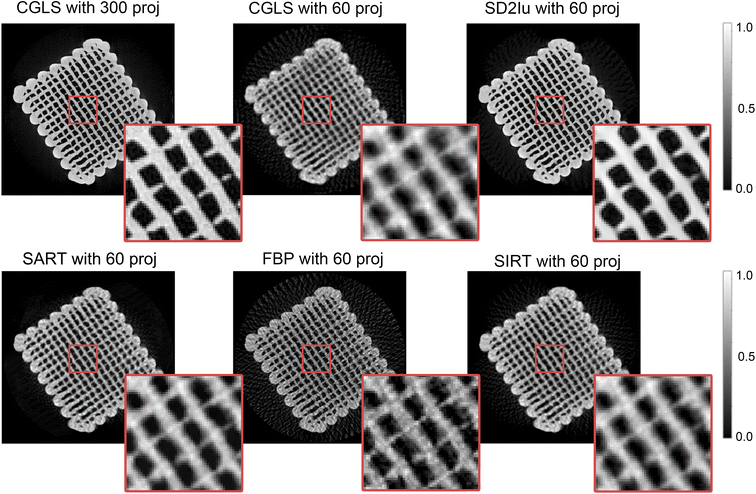Fig. 6 Photocatalyst XRD-CT image with the size of 331 × 331.⁵²

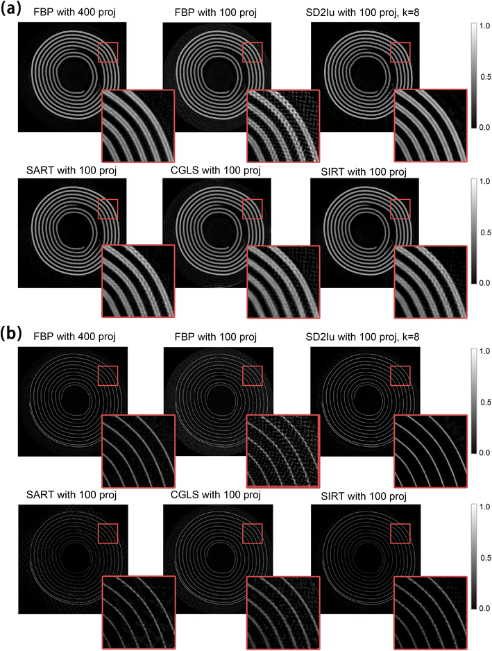
In Fig. 7 we show results from another XRD-CT dataset, using two larger sinograms selected from two diffraction peaks of interest (i.e. NMC532 and Cu phases respectively). This XRD-CT dataset was acquired using a commercially available 10440 NMC532 Li-ion battery.²⁵ The ground truth image was obtained using the CGLS algorithm on the 547 × 400 sinograms which already have fewer projections (i.e. 400 projections) than the Nyquist sampling theorem dictates (i.e. π/2 × 547). All the reconstruction algorithms and neural networks were tested using 547 × 100 sinograms which are severely undersampled data. As shown in Fig. 7, both reconstructed images indicate that the SD2I reconstructions have suppressed the angular undersampling artefacts while these are clearly present in the traditional methods.

Fig. 7 Two example XRD-CT reconstruction images: (a) chemical image corresponding to the NMC532 phase, (b) chemical image corresponding to the Cu phase. All SD2I results are using k factors equal to 8. The image sizes are 547 × 547. The SD2I and FBP results are reconstructed from the sinogram size as 547 × 100. The ground truth is obtained by the CGLS reconstruction of the 547 × 400 sinogram.

The metrics shown in Table 4 show that SD2I outperforms all other approaches but, as discussed previously, visual inspection and assessment of the reconstructed images is more important as there is no real ground truth image available for the experimental data. This is another advantage of the network compared to iterative approaches such as SART, SIRT and CGLS where there is no standard loss function one can use to calculate the optimal number of iterations (convergence criterion), especially when trying to reconstruct different datasets. The visual results clearly demonstrate that the SD2I reconstructions are considerably better quality than all other methods (FBP, CGLS, SART and SIRT) on the undersampled sinogram. Finally, it should be noted that, although the images have been normalised for better visualisation presentation, the SD2I, in contrast to other neural network reconstruction methods such as the GANrec, maintains the absolute intensity information which is essential in chemical tomography methods, such as XRD-CT. We tested two more experimental XRD-CT images with SD2Iu, which are shown in Fig. S9 and S10† with the metrics calculated in Tables S12 and S13.†

Table 4 Accuracy. Comparison of approaches for the example XRD-CT experimental images shown in Fig. 7. The CGLS with 400 projections is considered the ground truth. 250 iterations were used for the SART, SIRT and CGLS algorithms. Metrics were calculated using four significant figures

		FBP	SART	CGLS	SIRT	SD2Iu
(a)	MAE	0.3262	0.3310	0.3125	0.4563	0.1668
	MSE	0.3599	0.3333	0.2923	0.5881	0.1087
	SSIM	0.6632	0.7026	0.7197	0.6457	0.8265
	PSNR	23.21	23.55	24.12	21.08	28.414
(b)	MAE	0.6081	0.4630	0.4548	0.5141	0.3374
	MSE	1.525	0.9419	0.8539	1.299	0.5936
	SSIM	0.5276	0.6918	0.6753	0.6751	0.7472
	PSNR	20.79	22.88	23.31	21.48	24.89

---

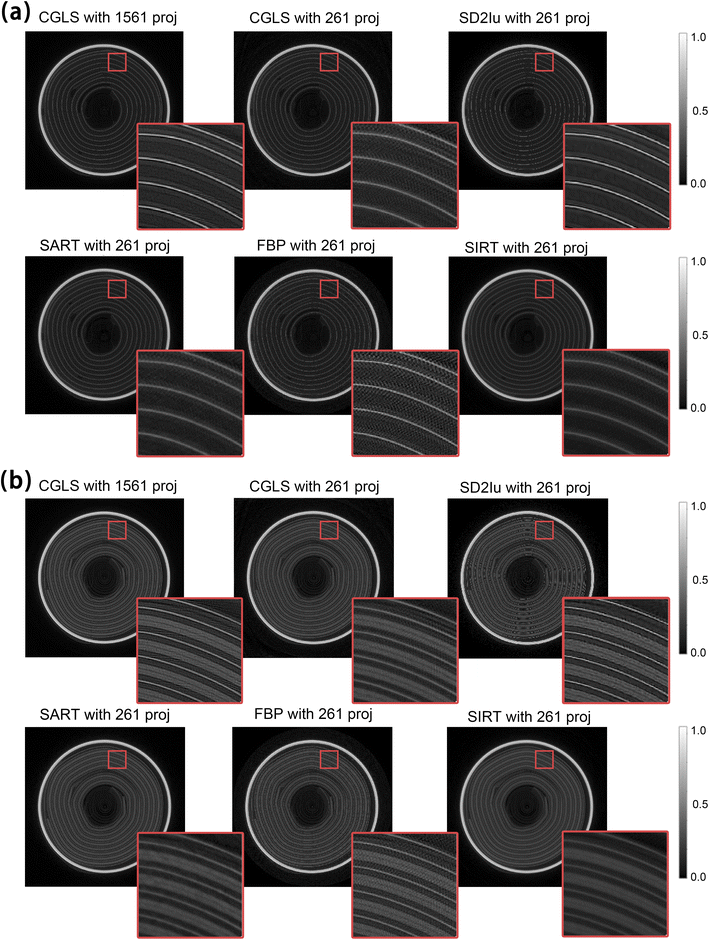
Fig. 8 and Table 5 present the results from the reconstructions of synchrotron X-ray micro-CT data acquired from the same 10440 NMC532 Li-ion battery corresponding to two different cross-sections. These two sinograms correspond to two different positions along the length of the battery (Fig. S11†); in position (a) only the Cu current collector is primarily visible in the battery jelly roll while in position (b) the NMC532 cathode can also be observed. As with the XRD-CT data above, ground-truth is obtained by CGLS of a full projection and the sinogram is then decreased to ¼ of the original size and reconstructions obtained with FBP, SD2I as well as the SIRT, CGLS and SART iterative methods. The hyperparameters for the SD2I networks used in this work for the micro-CT data were kept the same for all datasets and no tweaking was required (initial learning rate of 0.001 with a decaying rate and a safe margin of 8000 epochs).

Fig. 8 Two example micro-CT reconstruction images. All SD2I results are using k factors equal to 8. The image sizes are 779 × 779. The SD2I and FBP results are reconstructed from the sinogram size as 779 × 261. The ground truth is obtained by the CGLS reconstruction of the 779 × 1561 sinogram.

Table 5 Accuracy. Comparison of approaches for the example micro-CT experimental images shown in Fig. 8. The CGLS with 1561 projections is considered as the ground truth. Metrics calculated using four significant figures

		FBP	SART	CGLS	SIRT	SD2Iu
(a)	MAE	0.001724	0.001633	0.001596	0.001642	0.001146
	MSE	7.228 × 10^−6	9.044 × 10^−6	7.048 × 10^−6	1.042 × 10^−5	3.275 × 10^−6
	SSIM	0.6204	0.6678	0.6671	0.6711	0.7760
	PSNR	25.73	24.76	25.84	24.14	29.17
(b)	MAE	0.0004891	0.0004969	0.0004697	0.0005104	0.0003332
	MSE	5.546 × 10^−7	7.018 × 10^−7	5.494 × 10^−7	8.217 × 10^−7	2.636 × 10^−7
	SSIM	0.6903	0.6984	0.7191	0.6845	0.8371
	PSNR	26.52	25.49	26.56	24.81	29.74

---

As with the XRD-CT data, the SD2I reconstructions have fewer artefacts than the images obtained with all other methods. It is important to note here the image size; the resulting images are 779 × 779 pixels large. To the best of our knowledge, there is currently no other available self-supervised neural network that can perform direct reconstruction of such large sinograms/images without requiring a tremendous amount of GPU memory. We summarised the number of projections that the SD2Iu used to reconstruct the images shown in the paper and the number of projections that Nyquist sampling theorem dictates in Table S14.† Furthermore, in Fig. S12 and Table S15† we also show that the SD2I is able to reconstruct images with 1559 × 1559 pixels which demonstrates the scalability of this new architecture.

Summary and conclusions

We have presented a lightweight and scalable artificial neural network architecture, SD2I, for tomographic image reconstruction. The SD2I approach uses a generator network to produce a sample image, which is then converted to a sinogram via the Radon transform; the parameters of the network are updated by backpropagation to minimise the difference between the experimental sinogram and the sinogram produced by the network. Similar to other deep-learning reconstruction approaches, our SD2I approach is much more robust to angular undersampling than traditional reconstruction approaches. However, SD2I is also considerably more computationally efficient than other deep-learning reconstruction methods. This means the SD2I can be applied to much larger sinograms and can produce results with a significantly lighter hardware requirement than other deep-learning approaches. The advantages of the new architecture can be summarised as the following:

• Scalability: two new approaches in the architecture which radically reduce the number of parameters.

○ Single digit input.

○ Upsampling-type architecture after the last dense layer – this allows for decreasing the number of neurons in the last dense layer by a factor of at least 4.

• Ability to suppress angular undersampling artefacts which we demonstrated using both simulated and experimental data.

• Information regarding absolute intensities is maintained; the images are not normalised.

• Ease-of-use: the code can be run by a non-expert and does not require multiple hyperparameter tuning in contrast to other conventional methods (e.g. SART/SIRT/CGLS as well as regularisation-based methods).

• Simplicity: the addition of a discriminator network makes the training more complex and does not necessarily improve the resulting images (Fig. S13–S15 and Table S16†).

The ability to accurately reconstruct images from sparsely-sampled sinograms is critical for time-resolved in situ/operando tomography experiments as well as for reducing X-ray dose in medical CT. In its current form, the neural network cannot be compared to FBP in terms of speed but we have demonstrated its potential to suppress angular undersampling using real experimental data. Furthermore, the network could be potentially applied to other tomographic methods and modalities, such as neutron tomography and X-ray fluorescence tomography. Last but not least, the network has been developed for tomographic image reconstruction using 2D parallel/pencil beam geometries but we can foresee its application for other inverse problems in imaging if the appropriate forward model is known, such as the parallax problem in XRD-CT.

Methods

Experimental XRD-CT and micro-CT data

XRD-CT measurements of a commercial AAA Li-ion NMC532 Trustfire battery cell were performed at beamline station P07 of the DESY synchrotron using a 103.5 keV (λ = 0.11979 Å) monochromatic X-ray beam focused to have a spot size of 20 × 3 μm (H × V). 2D powder diffraction patterns were collected also using the Pilatus3 X CdTe 2 M hybrid photon counting area detector. The sample was mounted onto a goniometer which was placed on the rotation stage. The rotation stage was mounted perpendicularly to the hexapod; the hexapod was used to translate the sample across the beam. The XRD-CT scans were measured by performing a series of zigzag line scans in the z (vertical) direction using the hexapod and rotation steps. The XRD-CT scan was made with 550 translation steps (with a translation step size of 20 μm) covering 0–180° angular range, in 400 steps. The total acquisition time per point was 10 ms. XRD-CT measurements were also performed at beamline station ID15A of the ESRF⁵³ using a MnNaW/SiO₂ catalyst⁵⁴ and a 92.8 keV monochromatic X-ray beam focused to a spot size of 25 μm × 25 μm. 2D powder diffraction patterns were collected using a Pilatus3 X CdTe 300 K (487 × 619 pixels, pixel size of 172 μm) hybrid photon counting area detector. The acquisition time per point was 50 ms. The tomographic measurements were made with 180 translation steps covering 0–180° angular range, in steps of 1.5° (i.e. 120 line scans). XRD-CT measurements were performed at beamline ID15A of the ESRF using a 3D printed SrNbO2N photocatalyst⁵² and a 100 keV monochromatic X-ray beam focused to have a spot size of ca. 40 × 20 μm (horizontal × vertical). 2D powder diffraction patterns were acquired using the Pilatus3 X CdTe 2 M hybrid photon counting area detector. The XRD-CT scans were measured by performing a series of zigzag line scans. An exposure time of 10 ms and an angular range of 0–180° with 300 projections in total were used for the XRD-CT dataset. A translation step size of 100 microns was applied; in total 330 translation steps were made per line scan. Finally, XRD-CT measurements were made at beamline station ID31 of the ESRF using a Ni–Pd/CeO₂–ZrO₂/Al₂O₃ catalyst²¹ and a 70 keV monochromatic X-ray beam focused to have a spot size of 20 × 20 μm. Here, the total acquisition time per point was 20 ms. Tomographic measurements were made with 225 translation steps (translation step size of 20 μm) covering 0–180° angular range, in steps of 1.125° (i.e., 160 line scans). In each case, the detector calibration was performed using a CeO₂ standard. Every 2D diffraction image was calibrated and azimuthally integrated to a 1D powder diffraction pattern with a 10% trimmed mean filter using the pyFAI software package and the nDTomo software suite.^55,56 Sinograms of interest were extracted from the data volumes corresponding to the distribution of NMC532 and Cu battery cell components (AAA Li-ion NMC532), SrNbO2N (photocatalyst), NiO (Ni–Pd/CeO₂–ZrO₂/Al₂O₃ catalyst) and SiO₂ cristobalite (MnNaW/SiO₂ catalyst). Micro-CT measurements of the same commercial AAA Li-ion NMC532 Trustfire battery cell were performed at beamline station I12 of the Diamond Light Source using a 100 keV monochromatic X-ray beam. A PCO.edge X-ray imaging camera with 7.91 μm pixel size (beamline I12 module 2) was used for acquiring the radiographs during the CT scan. In total 1800 frames with an exposure time of 8 ms per frame during a 0–180° scan (angular step size of 0.1°). Each frame had a size of 2160 × 2560 pixels. Prior to the micro-CT scan, 50 dark current and flat field images were acquired which were used to normalise the radiographs prior to reconstruction. Two sinograms of interest were extracted from the data volume for the image reconstruction tests; each of these two sinograms was acquired after taking the mean of seven neighbouring sinograms (i.e. to increase the signal-to-noise ratio in the sinograms).

Data availability

All of the data and code used in this paper are publicly available through the following github repository which includes Google Colab notebooks to run the code: https://github.com/robindong3/SD2I.

Author contributions

H. D. designed and implemented the self-supervised reconstruction CNNs with contributions from A. V., K. T. B. and discussions with W. K. H. D. and A. V. prepared the SD2I python scripts and notebooks for the nDTomo software suite. H. D., A. V. and R. E. performed the various tests involving the reconstruction CNNs. S. W. T. P., R. E., Y. O. and A. G. were responsible for aspects of testing. A. V., D. M., Y. O., V. M., S. W. T. P., S. D. M. J. and A. M. B. designed the micro-CT and XRD-CT experiments and acquired the tomographic data. O. G., A. C. D. and M. Z. were responsible for P07 instrumentation and setup at the PETRA III, DESY. H. D., A. V. and K. T. B. are responsible for writing the manuscript with feedback given by all co-authors.

Conflicts of interest

The authors declare no conflicts of interest.

Acknowledgements

Finden acknowledges funding through Harwell Campus Cross-Cluster Proof of Concept (POC) projects POC2020-07 “Super-resolution in neutron tomography” and POC2021-10 “Accelerating neutron tomography with applied deep learning”. We would like to thank Graham Appleby for discussions during the Harwell Campus Cross-Cluster POC projects. We would like to thank Leigh Connor (Diamond Light Source) for preparing I12 beamline instrumentation and setup and for his help with the micro-CT data acquisition. We acknowledge DESY (Hamburg, Germany), a member of the Helmholtz Association HGF, for the provision of experimental facilities. Parts of this research were carried out at PETRA III. We would like to thank ESRF for beamtime as well as Marco di Michiel (ID15A, ESRF) and Jakub Drnec (ID31, ESRF) for preparing beamline instrumentation and setup and for their help with the experimental XRD-CT data acquisition. K. T. B., A. V. and S. D. M. J. acknowledge funding from the AI3SD program (AI3SD-FundingCall2 017). A. M. B. acknowledges EPSRC (grants EP/R026815/1 and EP/S016481/1). A. V. acknowledges financial support from the Royal Society as a Royal Society Industry Fellow (IF\R2\222059).

References

1. M. Prosperi, et al., Causal inference and counterfactual prediction in machine learning for actionable healthcare, Nature Machine Intelligence, 2020, 2, 369–375.
2. H. Altae-Tran, B. Ramsundar, A. S. Pappu and V. Pande, Low Data Drug Discovery with One-Shot Learning, ACS Cent. Sci., 2017, 3, 283–293.
3. K. T. Butler, D. W. Davies, H. Cartwright, O. Isayev and A. Walsh, Machine learning for molecular and materials science, Nature, 2018, 559, 547–555.
4. D. W. Davies, et al., Computer-aided design of metal chalcohalide semiconductors: from chemical composition to crystal structure, Chem. Sci., 2018, 9, 1022.
5. B. Zhu, J. Z. Liu, S. F. Cauley, B. R. Rosen and M. S. Rosen, Image reconstruction by domain-transform manifold learning, Nature, 2018, 555, 487–492.
6. J. Choe, et al., Deep Learning–Based Image Conversion of CT Reconstruction Kernels Improves Radiomics Reproducibility for Pulmonary Nodules Or Masses, Radiology, 2019, 292, 365–373.
7. K. H. Jin, M. T. McCann, E. Froustey and M. Unser, Deep Convolutional Neural Network for Inverse Problems in Imaging, IEEE Trans. Image Process., 2017, 26, 4509–4522.
8. M. J. Willemink and P. B. Noël, The evolution of image reconstruction for CT-from filtered back projection to artificial intelligence, Eur. Radiol., 2019, 29, 2185–2195.
9. H.-M. Zhang and B. Dong, A Review on Deep Learning in Medical Image Reconstruction, Journal of the Operations Research Society of China, 2020, 8, 311–340.
10. A. F. Rodriguez, W. E. Blass, J. H. Missimer and K. L. Leenders, Artificial neural network Radon inversion for image reconstruction, Med. Phys., 2001, 28, 508–514.
11. P. Paschalis, et al., Tomographic image reconstruction using Artificial Neural Networks, Nucl. Instrum. Methods Phys. Res., Sect. A, 2004, 527, 211–215.
12. M. Argyrou, D. Maintas, C. Tsoumpas and E. Stiliaris, Tomographic Image Reconstruction Based on Artificial Neural Network (ANN) Techniques, in 2012 IEEE Nuclear Science Symposium and Medical Imaging Conference Record (NSS/MIC), 2012, pp. 3324–3327,  DOI:10.1109/NSSMIC.2012.6551757.
13. T. Würfl, F. C. Ghesu, V. Christlein and A. Maier, Deep Learning Computed Tomography, in Medical Image Computing and Computer-Assisted Intervention – MICCAI 2016, ed. S. Ourselin, L. Joskowicz, M. R. Sabuncu, G. Unal and W. Wells, Springer International Publishing, 2016, pp. 432–440.
14. Y. Ge, et al., ADAPTIVE-NET: deep computed tomography reconstruction network with analytical domain transformation knowledge, Quant. Imag. Med. Surg., 2020, 10, 415–427.
15. G. Ma, Y. Zhu and X. Zhao, Learning Image from Projection: A Full-Automatic Reconstruction (FAR) Net for Computed Tomography, IEEE Access, 2020, 8, 219400–219414.
16. X. Yang and C. Schroer, Strategies of Deep Learning for Tomographic Reconstruction, in 2021 IEEE International Conference on Image Processing (ICIP), 2021, pp. 3473–3476,  DOI:10.1109/ICIP42928.2021.9506395.
17. A. M. Beale, S. D. M. Jacques, E. K. Gibson and M. Di Michiel, Progress towards five dimensional diffraction imaging of functional materials under process conditions, Coord. Chem. Rev., 2014, 277–278, 208–223.
18. S. Das, R. Pashminehazar, S. Sharma, S. Weber and T. L. Sheppard, New Dimensions in Catalysis Research with Hard X-Ray Tomography, Chem. Ing. Tech., 2022, 94, 1591–1610.
19. P. P. Paul, et al., A Review of Existing and Emerging Methods for Lithium Detection and Characterization in Li-Ion and Li-Metal Batteries, Adv. Energy Mater., 2021, 11, 2100372.
20. H. Matsui, et al., Operando 3D Visualization of Migration and Degradation of a Platinum Cathode Catalyst in a Polymer Electrolyte Fuel Cell, Angew. Chem., Int. Ed., 2017, 56, 9371–9375.
21. A. Vamvakeros, et al., 5D operando tomographic diffraction imaging of a catalyst bed, Nat. Commun., 2018, 9, 4751.
22. D. Matras, et al., Multi-length scale 5D diffraction imaging of Ni–Pd/CeO₂–ZrO₂/Al₂O₃ catalyst during partial oxidation of methane, J. Mater. Chem. A, 2021, 9, 11331–11346.
23. I. Martens, et al., Imaging Heterogeneous Electrocatalyst Stability and Decoupling Degradation Mechanisms in Operating Hydrogen Fuel Cells, ACS Energy Lett., 2021, 6, 2742–2749.
24. J. Becher, et al., Chemical gradients in automotive Cu-SSZ-13 catalysts for NO_x removal revealed by operando X-ray spectrotomography, Nat. Catal., 2021, 4, 46–53.
25. A. Vamvakeros, et al., Cycling Rate-Induced Spatially-Resolved Heterogeneities in Commercial Cylindrical Li-Ion Batteries, Small Methods, 2021, 5, 2100512.
26. D. Matras, et al., Emerging chemical heterogeneities in a commercial 18650 NCA Li-ion battery during early cycling revealed by synchrotron X-ray diffraction tomography, J. Power Sources, 2022, 539, 231589.
27. A. Beck and M. Teboulle, Fast Gradient-Based Algorithms for Constrained Total Variation Image Denoising and Deblurring Problems, IEEE Trans. Image Process., 2009, 18, 2419–2434.
28. D. M. Pelt and K. J. Batenburg, Fast Tomographic Reconstruction from Limited Data Using Artificial Neural Networks, IEEE Trans. Image Process., 2013, 22, 5238–5251.
29. E. Bladt, D. M. Pelt, S. Bals and K. J. Batenburg, Electron tomography based on highly limited data using a neural network reconstruction technique, Ultramicroscopy, 2015, 158, 81–88.
30. J. He, Y. Wang and J. Ma, Radon Inversion via Deep Learning, IEEE Trans. Med. Imaging, 2020, 39(6), 2076–2087.
31. T. Würfl, et al., Deep Learning Computed Tomography: Learning Projection-Domain Weights from Image Domain in Limited Angle Problems, IEEE Trans. Med. Imag., 2018, 37, 1454–1463.
32. X. Yang, et al., Low-dose X-ray tomography through a deep convolutional neural network, Sci. Rep., 2018, 8, 2575.
33. H. Yuan, J. Jia and Z. Zhu, SIPID: a deep learning framework for sinogram interpolation and image denoising in low-dose CT reconstruction, in 2018 IEEE 15th International Symposium on Biomedical Imaging (ISBI 2018), 2018, pp. 1521–1524,  DOI:10.1109/ISBI.2018.8363862.
34. J. Dong, J. Fu and Z. He, A deep learning reconstruction framework for X-ray computed tomography with incomplete data, PLoS One, 2019, 14, 1–17.
35. D. Bellos, M. Basham, T. Pridmore and A. P. French, A convolutional neural network for fast upsampling of undersampled tomograms in X-ray CT time-series using a representative highly sampled tomogram, J. Synchrotron Radiat., 2019, 26, 839–853.
36. D. M. Pelt, K. J. Batenburg and J. A. Sethian, Improving Tomographic Reconstruction from Limited Data Using Mixed-Scale Dense Convolutional Neural Networks, J. Imaging, 2018, 4, 128.
37. D. M. Pelt and J. A. Sethian, A mixed-scale dense convolutional neural network for image analysis, Proc. Natl. Acad. Sci. U. S. A., 2018, 115, 254–259.
38. Y. Ge, et al., Deconvolution-Based Backproject-Filter (BPF) Computed Tomography Image Reconstruction Method Using Deep Learning Technique, 2018,  DOI:10.48550/ARXIV.1807.01833.
39. X. Yang, et al., Tomographic reconstruction with a generative adversarial network, J. Synchrotron Radiat., 2020, 27, 486–493.
40. Z. Liu, et al., TomoGAN: Low-Dose Synchrotron X-Ray Tomography with Generative Adversarial Networks, J. Opt. Soc. Am. A, 2020, 37, 422.
41. Z. Wu, A. Alorf, T. Yang, L. Li and Y. Zhu, Robust X-ray Sparse-view Phase Tomography via Hierarchical Synthesis Convolutional Neural Networks, ArXiv190110644 Cs, 2019.
42. Learning with known operators reduces maximum error bounds | Nature Machine Intelligence, https://www.nature.com/articles/s42256-019-0077-5.
43. S. R. Daemi, et al., Exploring cycling induced crystallographic change in NMC with X-ray diffraction computed tomography, Phys. Chem. Chem. Phys., 2020, 22, 17814–17823.
44. D. Matras, et al., Effect of thermal treatment on the stability of Na–Mn–W/SiO₂ catalyst for the oxidative coupling of methane, Faraday Discuss., 2021, 229, 176–196.
45. Z. Wang, A. C. Bovik, H. R. Sheikh and E. P. Simoncelli, Image quality assessment: from error visibility to structural similarity, IEEE Trans. Image Process., 2004, 13, 600–612.
46. A. Karnewar, AANN: Absolute Artificial Neural Network, in 2018 3rd International Conference for Convergence in Technology (I2CT), IEEE, 2018, pp. 1–6.
47. O. I. Berngardt, Improving Classification Neural Networks by Using Absolute Activation Function (MNIST/LeNET-5 Example), ArXiv Prepr. ArXiv230411758, 2023.
48. D. P. Kingma and J. Ba, Adam: A Method for Stochastic Optimization, 2014,  DOI:10.48550/ARXIV.1412.6980.
49. H. Zhao, O. Gallo, I. Frosio and J. Kautz, Loss Functions for Neural Networks for Image Processing, 2015,  DOI:10.48550/ARXIV.1511.08861.
50. M. Abadi, et al., TensorFlow: Large-Scale Machine Learning on Heterogeneous Systems, 2015.
51. W. v. Aarle, et al., The ASTRA Toolbox: a platform for advanced algorithm development in electron tomography, Ultramicroscopy, 2015, 157, 35–47.
52. A. Iborra-Torres, et al., 3D printed SrNbO2N photocatalyst for degradation of organic pollutants in water, Mater. Adv., 2023 10.1039/D2MA01076C.
53. G. B. M. Vaughan, et al., ID15A at the ESRF – a beamline for high speed operando X-ray diffraction, diffraction tomography and total scattering, J. Synchrotron Radiat., 2020, 27, 515–528.
54. A. Vamvakeros, et al., Real-time multi-length scale chemical tomography of fixed bed reactors during the oxidative coupling of methane reaction, J. Catal., 2020, 386, 39–52.
55. A. Vamvakeros, et al., Removing multiple outliers and single-crystal artefacts from X-ray diffraction computed tomography data, J. Appl. Crystallogr., 2015, 48, 1943–1955.
56. A. Vamvakeros, nDTomo software suite, 2019, DOI: https://doi.org/10.5281/zenodo.7139214, https://github.com/antonyvam/nDTomo.

---

Footnote

† Electronic supplementary information (ESI) available. See DOI: https://doi.org/10.1039/d2dd00105e

---