
 Open Access Article
 This Open Access Article is licensed under a
 Creative Commons Attribution 3.0 Unported Licence
Predicting pharmaceutical powder flow from microscopy images using deep learning
Matthew R.
Wilkinson
 *abc,
Laura
Pereira Diaz
d,
Antony D.
Vassileiou
d,
John A.
Armstrong
d,
Cameron J.
Brown
d,
Bernardo
Castro-Dominguez
abc and
Alastair J.
Florence
*d
*abc,
Laura
Pereira Diaz
d,
Antony D.
Vassileiou
d,
John A.
Armstrong
d,
Cameron J.
Brown
d,
Bernardo
Castro-Dominguez
abc and
Alastair J.
Florence
*d
aDepartment of Chemical Engineering, University of Bath, Claverton Down, Bath BA2 7AY, UK. E-mail: mrw39@bath.ac.uk
bEPSRC Future Continuous Manufacturing and Advanced Crystallisation Research Hub (CMAC), University of Bath, Claverton Down, Bath BA2 7AY, UK
cCentre for Sustainable and Circular Technologies (CSCT), University of Bath, Claverton Down, Bath BA2 7AY, UK
dEPSRC Future Continuous Manufacturing and Advanced Crystallisation Research Hub, c/o Strathclyde Institute of Pharmacy and Biomedical Sciences, University of Strathclyde, Glasgow, UK. E-mail: alastair.florence@strath.ac.uk
First published on 13th February 2023
Abstract
The powder flowability of active pharmaceutical ingredients and excipients is a key parameter in the manufacturing of solid dosage forms used to inform the choice of tabletting methods. Direct compression is the favoured tabletting method; however, it is only suitable for materials that do not show cohesive behaviour. For materials that are cohesive, processing methods before tabletting, such as granulation, are required. Flowability measurements require large quantities of materials, significant time and human investments and repeat testing due to a lack of reproducible results when taking experimental measurements. This process is particularly challenging during the early-stage development of a new formulation when the amount of material is limited. To overcome these challenges, we present the use of deep learning methods to predict powder flow from images of pharmaceutical materials. We achieve 98.9% validation accuracy using images which by eye are impossible to extract meaningful particle or flowability information from. Using this approach, the need for experimental powder flow characterization is reduced as our models rely on images which are routinely captured as part of the powder size and shape characterization process. Using the imaging method recorded in this work, images can be captured with only 500 mg of material in just 1 hour. This completely removes the additional 30 g of material and extra measurement time needed to carry out repeat testing for traditional flowability measurements. This data-driven approach can be better applied to early-stage drug development which is by nature a highly iterative process. By reducing the material demand and measurement times, new pharmaceutical products can be developed faster with less material, reducing the costs, limiting material waste and hence resulting in a more efficient, sustainable manufacturing process. This work aims to improve decision-making for manufacturing route selection, achieving the key goal for digital design of being able to better predict properties while minimizing the amount of material required and time to inform process selection during early-stage development.
1 Introduction
Powder flowability represents a key property that influences the performance of the materials in pharmaceutical manufacturing. Direct compression is the preferred manufacturing technique by pharmaceutical companies to make tablets, but this technique has high requirements regarding powder flow. Particularly when doing batch processing, only materials with sufficiently good flow properties can be compacted into tablets.1 Although the literature shows that continuous direct compression is more tolerant to cohesive materials; understanding the flow properties of the material remains a critical consideration, especially as continuous processes are newer technologies that are still being adopted.2,3 In the context of this work, we focus on batch processes but highlight continuous processes as important future study. Where less desirable properties are present, poor powder flow can: lead to challenges during blending (no discharge or ratholing),4 difficulties when discharging the powder into the hopper5 or issues regarding weight uniformity in the tablet.6 Therefore, a material that has poor powder flow needs to be pre-processed before attempting direct compression.7–9 The most common pre-processing step used before compression is granulation, which is needed to ensure that the final formulation can then be compressed into a tablet.The flowability of a given pharmaceutical powder is a multivariate phenomenon. There are many methods that can be used to measure different powder properties that contribute to the overall flowability.10,11 Factors which affect flowability include particle size, particle shape, density and surface area, as well as environmental factors such as moisture levels.12 As there are so many factors, it is challenging to use a single test which captures a complete profile of the flow behaviour.8 To effectively use these contributing factors as features for modelling, they must be able to be measured accurately and ideally reasonably quickly.
Currently, to measure powder flowability, there are multiple methods available as presented by Tan et al.13. Examples include: (1) powder densities and their indices such as Carr's index which is a measure of compressibility and the Hausner ratio which is the quotient of the tapped and bulk densities. (2) Avalanching, where powder is rotated in a cylindrical apparatus and a camera records flow behaviour. (3) Angle of repose (AOR), which is the angle between the horizontal plane and the free sloping side of the cone-like shape that forms when powders are dropped from a small height. (4) Time to flow through an orifice or the critical diameter needed to flow through. (5) Sheer cell testers such as the FT4 Powder Rheometer, which measure the torque needed to constantly rotate a blade through a material and gives flow function coefficient (FFc) values. These experimental analyses present several disadvantages, i.e. large experimental error, low reproducibility, and time and resource consumption.14 These disadvantages highlight the need for alternative methods to predict powder flowability to save time and resources, especially at the beginning of the development of a new pharmaceutical ingredient, when the amount of material available is at its premium. By compiling and using training data that is the result of this rigorous process of repeat testing, we ensure that the ground truth labels are accurate and hence the predictions made by the Deep Learning (DL) models and the trends which the networks capture are too. Once these trends are modelled, users can significantly reduce the demand for repeat testing as the predictions incorporate this prior experience.
Previous studies in the literature create models to predict powder flow from particle shape and size analysis. It is widely accepted that particle size and shape have a significant impact on flowability. Usually coarser and spherical particles will have better flow properties.15,16 Yu et al.17 used partial least squares analysis to generate numerical descriptors corresponding to particle shape and size, successfully estimating FFc and stating that the most important variables for the prediction of powder flow were the diameter descriptors of the particles and the aspect ratio. They therefore emphasized the importance of considering multiple descriptors to characterize powder flow. Most recently, Barjat et al.18 used statistical modelling to infer trends from numerical values calculated as a result of analytical methods, demonstrating the feasibility of the prediction of powder flow of pharmaceutical powders from particle physical properties.
In this work, we present a novel approach to solving this problem. DL models were used to analyze images of bulk powder particles and classify their flowability as either cohesive, easy flowing or free-flowing, based on their FFc (smaller than 4, between 4 and 10, or greater than 10, respectively), following Jenike's classification system.19 Using DL models delivers significant advantages over existing modelling approaches. These include autonomous feature extraction and removing the need for manual parameterization of particle size and shape using “human-made” descriptors. Furthermore, the implementation of such models would reduce the time and amount of material required for the characterization of powder flow. In this work we were able to reduce our resource costs from 2 hours and 30 g to 1 hour and 500 mg for each measurement. Particle shape and size characterization already forms an integral part of the manufacturing process. Hence, by developing a method where additional information can be extracted from existing measurements using DL, additional value is added to an existing test. After the initial time investment to train a DL network on suitably large datasets, experimental flow testing can be omitted, offering the most significant time saving. The authors note that recording accurate measurement times can be challenging especially when users with different setups and equipment are taking measurements and so the reduction in material is, at present, likely more significant than the time savings recorded in this study. Overall this dramatically reduces the resource demand and cost associated with the screening of new products. As a result of the proposed predictive model, users will experience shorter development timelines, leading to a more efficient and sustainable manufacturing approach.
2 Materials and methods
The source code and dataset for the entirety of this work have been made available online at https://github.com/MRW-Code/cmac_particle_flow. A full list of the raw materials used and their respective suppliers is included in Appendix A. All materials were used as obtained without any further treatment. All of the FFc values are listed with the corresponding individual or mixture of raw materials in Appendix B.2.1 Image data collection
The dataset has a total of 99 images; from these 30 were pure materials and 69 images correspond to binary or multi-component pharmaceutical mixtures. The images were generated using Malvern Morphologi G3 particle characterization system (Malvern Panalytical, Malvern, UK). The operating procedure for the Morphologi G3 was designed to be consistent across samples, to give reproducible images that were not affected by experimental factors. This technique is a static imaging method where images are captured across multiple focal planes and compiled into larger composite images an example of which is shown in Fig. 4. 500 mg of each material was dispersed onto the glass plate with an injection pressure of 0.8 bar for 20 milliseconds and then given a 1 minute settling time. A 5× optic selection was used and to remove overlapping particles the overlap setting and threshold intensity were set to 40% and 105, respectively. A trash size of 10 pixels was used to remove noise. No filters, segmentation methods, hole-filling or classification settings were used.After the measurement using the Morphologi G3, the area composite was scanned to obtain an overall image. The software created a composite image by tiling together all the individual frames taken during the measurement to collect them in a single image of the scanned area. From this composite image, a maximum reproducible crop of 5359 × 3491 pixels was taken to ensure consistent sizing of images from different samples. An example of these images is shown in Fig. 1.
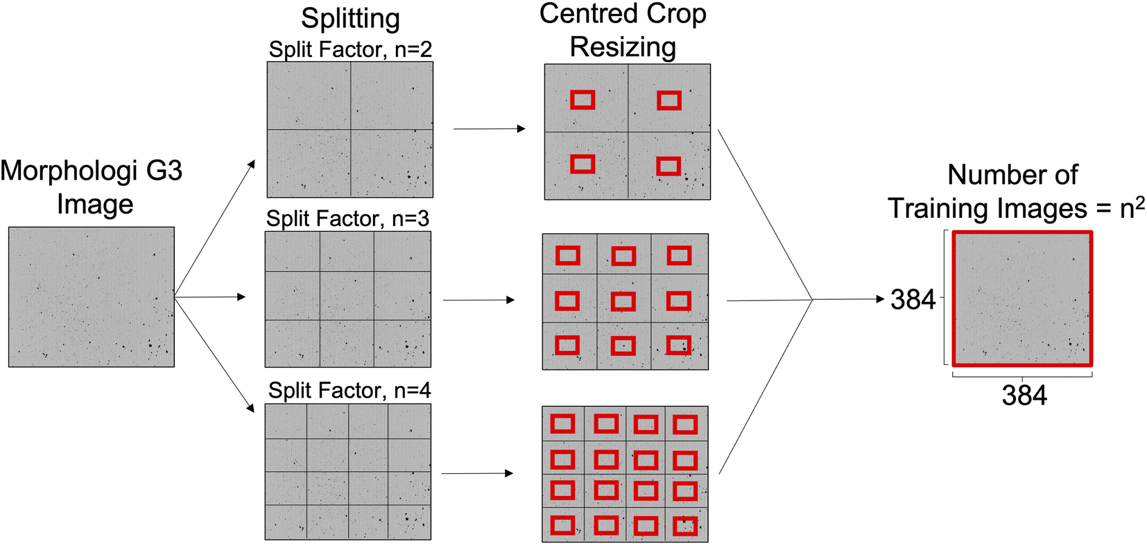 | ||
| Fig. 1 Splitting and resizing of the raw Morphologi G3 images to give n2 training images. Figure not to scale, split factor = 2, 3 & 4 shown for illustration purposes. | ||
Literature offers some guidance for the minimum number of particles needed for representative measurements of particle properties. For example, Almeida-Prieto et al.20 suggest 300 particles are needed for morphology characterization and Pons et al.21 suggest ideally 1000–1500. Although not direct standards for flow prediction, as we aimed to use particle size and shape for prediction these offer good guidelines. During the experimental flowability measurements, the mean number of particles in each image was 83503 and the median was 30165. No samples had fewer than 300 particles, with the minimum being 332. Furthermore, only 3 samples had fewer than 1000 particles. As such, all of the samples in the dataset were indeed considered representative. There are no literature standards for how many particles must be imaged to accurately predict particle flow from microscopy images. Although morphology standards suggest the samples were representative; we explicitly investigated reducing the number of particles by cropping the images to explore how it affected overall model accuracy.
2.2 Bulk property measurements
To label training examples, a Freeman FT4 Powder Rheometer was used to measure the powder flow behaviour using the shear cell test. The vessel selected was the 25 mm × 10 ml borosilicate split vessel. The first step was the conditioning cycle, performed by the 23.5 mm stainless-steel blade which rotated clockwise, downwards and upwards on a vertical axis through the powder, establishing a flow pattern by generating a movement with the interaction of the particles. Once the powder was conditioned, the 23.5 mm blade was swapped by the compaction piston for axial compression. The piston compacts the powder at an initial normal stress of 9 kPa. After the powder was been consolidated, the excess was removed from the vessel by splitting it in two.A shear cell test was used to calculate the FFc of the powders. A control normal stress was applied, and the shearing induced rotation. The output data was the representation of the relationship between the shear stress and the normal stress, which defines the powder's yield locus. Following Jenike's classification, powders with a FFc below 4 have poor flow; between 4 and 10, they are fairly flowable; and above 10, free-flowing. Based on this classification, the powders were classified into cohesive, easy flowing or free-flowing, respectively.19
2.3 Data pre-processing and augmentation
Raw images from the Morphologi G3 were 5359 × 3491 pixels. Images of this size are impractical for DL as they demand a significant memory overhead which restricts the batch size and model depth, as well as increasing the training time. As such, the raw images were split and resized into smaller crops as shown in Fig. 1. This process is best described as defining how many unique 384 × 384 tiles to take from every raw Morphologi G3 image, which was an important hyperparameter in this work.The number of splits was controlled by defining a split factor, n. The number of crops taken from the raw Morphologi G3 image is calculated as n2 when n ≥ 2. When n = 1, images were split in half and when n = 0, the raw image remained unchanged. After splitting, each of the resulting crops were resized using the centred crop method built into the fastai library, in order to preserve the aspect ratio.22 These centred crops were of size 384 × 384 pixels, which was chosen to mimic the pre-trained Vision Transformer (ViT) image inputs which have been made publicly available.23 Split index values greater than 10 were not tested. This was because splitting beyond n = 10 generated images smaller than 384 × 384 pixels and so padding must be used which is wasted computation as it contains no information about particle features pertinent to flowability. To determine if the resizing was in itself limiting, an evaluation was also carried out without it, leaving the images at their native “after splitting” pixel sizes. This was an isolated test and hence unless otherwise clearly stated, the resizing was always used.
Data augmentations are common practice across applications of DL to provide larger and more diverse training data using label preserving transforms.24 Augmentations allow models to better generalise and reduce the risk of overfitting by helping models learn underlying patterns instead of memorising training examples. In this study, the augmentation strategy was designed to maximise the trends which can be inferred from each data point without creating synthetic particle data that does not exist in the samples. Other work has shown the use of generative networks to create synthetic data; however, this was not explored in this case.25 In this work, augmentations were used to account for the random particle dispersion during imaging by exposing the network to particles in different positions and orientations. This ensures that predictions are a result of the particle properties instead of translational effects. For example, the rotation of a particle does not change the fundamental particle properties. Yet, it is almost certain that if sprayed onto a plate again (as is done in the Morphologi G3 imaging), the particle would orient itself differently, so the model must account for this. This ultimately improves performance and is especially powerful when access to large datasets is limited.26 In an industrial setting, with access to proprietary datasets, combining augmentations with continuous data integration will help deliver the resilience necessary for product quality assurance and process control.
As shown in Fig. 2, the resulting cropped images were subjected to 2 × 90° rotations up to 180° and then a single flip was applied along both the horizontal and vertical axes simultaneously. Warping and deletion style augmentations were deliberately excluded. In the warping case, this was to avoid changing the particle shape as this is known to be a contributing factor to the flow function. Deletions were not used so that particles were not removed from the images beyond that which were already lost from cropping. Cropping the raw Morphologi G3 images was carried out for all data, but the additional augmentations were only applied to the training set.
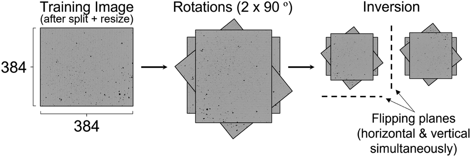 | ||
| Fig. 2 Rotation and inversion operations used to augment the training images. | ||
2.4 Network architecture and training
In this work, 4 different computer vision DL architectures were tested, as listed.(1) ResNet18 (ref. 27)
(2) Vision Transformer (ViT)28
(3) SWIN Transformer V2 (SWIN-V2)29,30
(4) ConvNeXt31
These architectures were chosen as they each incorporate different blocks that have been previously demonstrated as effective in image processing tasks, namely convolution and attention. The ResNet18 architecture represents a purely convolutional model which has been dominant over recent years for image processing. Despite this literature dominance, more recently, the rise of transformer models and the attention mechanism has prompted the development of models capable of applying these newer methods to images. As such, in this work we also tested the ViT and SWIN-V2 models to represent attention-based architectures. The difference between the two transformer models is attributed to the application of the attention mechanism. The ViT applies global attention and so the input size must be fixed. In contrast, SWIN applies attention locally by using a sliding window, and as such the input sizes can be more flexible. Most recently of all, the ConvNeXt model was published which reevaluates and ultimately improves on purely convolutional approaches, bringing them in line with the competition from transformer architectures. In their respective publications, each model has strong performance metrics and so there was no obvious candidate that is applicable across all vision applications. Hence, we evaluated each model to see which approach yielded superior results for the classification of flowability. All models were downloaded with pre-trained weights from PyTorch image models (timm).23 Implementation used the PyTorch and fastai python packages.22,32
During testing, each of the listed networks were trained using a transfer learning approach, pre-loading weights from ImageNet, before fine-tuning two final fully connected layers for classifying particle flow.33 A grid search was carried out to determine optimal hyperparameters which informed the values listed in the training details that follow. The dataset was split into batches, and the models were trained using an early stopping mechanism to prevent overfitting. The early stopping mechanism monitored the validation loss and stopped the training process once it failed to decrease over the previous 5 epochs. After stopping, the model with the lowest validation loss was saved and used for inference. All models were trained on a single Nvidia RTX 3090 GPU with 24 GB of VRAM. To assess the potential for batch sizes beyond what the memory allocation allowed, gradient accumulation was used. Gradient accumulation allows a specified number of batches to pass through the network before pooling their gradients for use during the backpropagation of errors to update the model weights. As a result, we could overcome memory limitations and train the model such that the effective batch size was equal to the product of the actual batch size and the number of gradient accumulation steps.
The authors acknowledge that during this work there were cases where the centred crop was not used. In these cases, the demand for high VRAM resources may present a barrier to entry in reproducing this work. However, when the centred crop is used, and by taking advantage of gradient accumulation where appropriate, the memory requirement can be significantly reduced and hence these models can be reproduced without the need for such high-end hardware resources.
2.5 Evaluation
The model was evaluated using a 5-fold stratified cross-validation strategy to split into training, validation and testing subsets in an 80![[thin space (1/6-em)]](https://www.rsc.org/images/entities/char_2009.gif) :10:10 ratio. The stratified approach to splitting was implemented using scikit-learn to ensure that the ratio of samples in each class remained constant across all subsets.34 Furthermore, when curating the dataset, it was ensured that the number of samples in each class remained as close to equal as was practically possible to avoid misinterpretation of validation metrics due to class imbalance issues. The number of samples in every class is shown in Table 1. Selecting the samples to be used in the external test set was random.
:10:10 ratio. The stratified approach to splitting was implemented using scikit-learn to ensure that the ratio of samples in each class remained constant across all subsets.34 Furthermore, when curating the dataset, it was ensured that the number of samples in each class remained as close to equal as was practically possible to avoid misinterpretation of validation metrics due to class imbalance issues. The number of samples in every class is shown in Table 1. Selecting the samples to be used in the external test set was random.
| Class | FFc | Number of materials |
|---|---|---|
| Cohesive | ≤4 | 30 |
| Easy flowing | 4 < FFc < 10 | 34 |
| Free flowing | ≥10 | 35 |
The 5 fold cross-validation was used to ensure that performance metrics were further not misrepresented by favourable seeding of the random data splits in a particular training example. Each experiment was repeated 3 times, and the presented metrics represent a mean of these repeats, with standard deviation errors included where appropriate as error bars. The dataset was split into train/validation/test subsets before any pre-processing or cropping steps were applied. This ensured no data leakage occurred where crops of the same image were present in both the training and validation/test sets. Furthermore, defining data splits before the raw Morphologi G3 images were split or cropped guaranteed that the validation and test set only contained entirely unseen bulk powders.
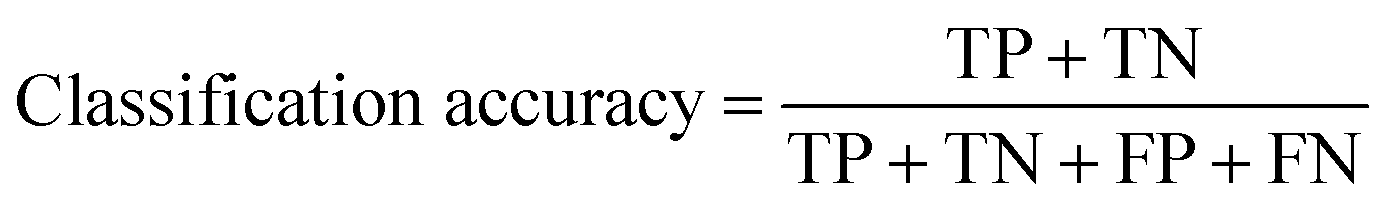
After assessing the validation accuracy, the external test set was used to ensure the model was not overfitting either of the training or validation sets while also representing a deployment scenario. At test time, the metrics were calculated using two approaches. (1) “Single”, where all crops were considered as unique images. (2) “Majority”, which used an ensemble approach to consider the predictions across all the crops from a given original Morphologi G3 image, and assigned a label as the most commonly predicted class. Despite the majority vote being the favoured approach from a deployment perspective, both methods were used to maximise the interpretability of the models. Performance was evaluated using classification accuracy as the primary metric, which was calculated using eqn (1), where TP, FP, TN, FN are true positive, false positive, true negative and false negative, respectively. In addition to this, the confusion matrices were also recorded.
 | (1) |
3 Results and discussion
3.1 Experimental powder measurements
The powder behaviour class was assigned to each image based on the results obtained using the powder rheometer. The results of the samples analysed are gathered in Table 1. Thus, 31 powders belonged to the “Cohesive” class, 35 powders belonged to the “Easy flowing” class and the remaining 33 powders belonged to the “Free flowing” class. An example of the images that were captured using the Morphologi G3 is shown in Fig. 3.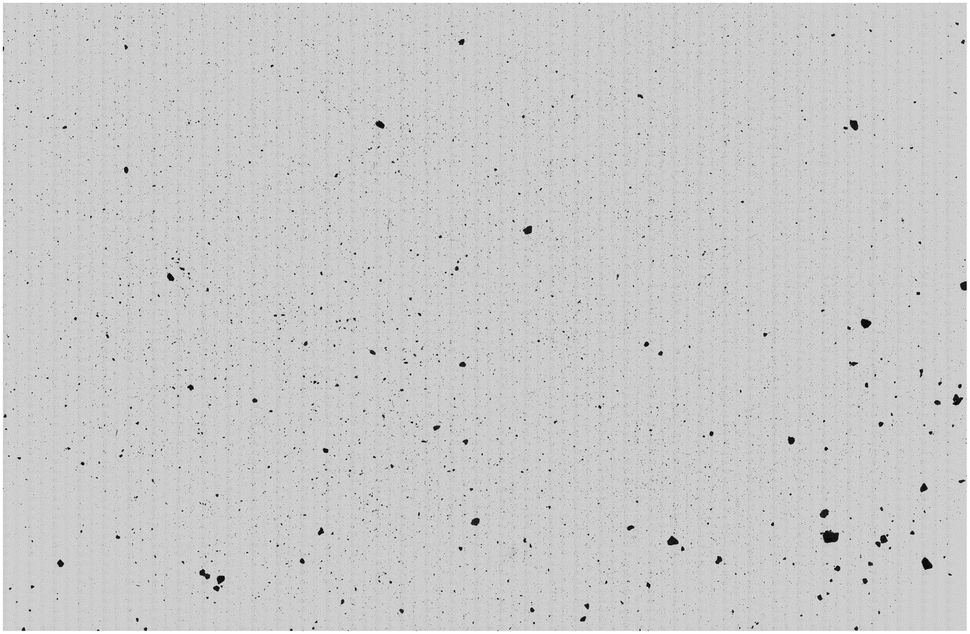 | ||
| Fig. 3 Full resolution (5359 × 3491 pixels) image of caffeine captured using the Morphologi G3. | ||
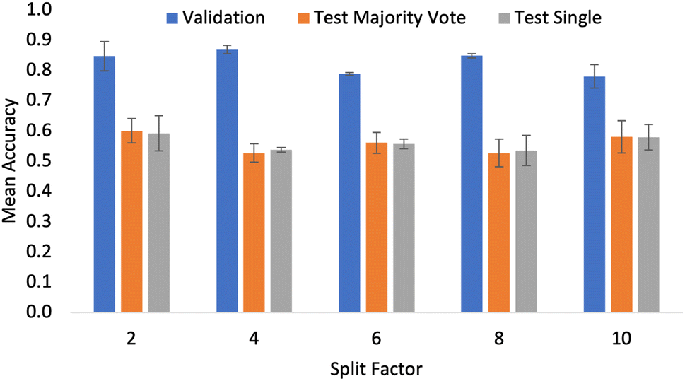 | ||
| Fig. 4 Mean classification accuracy across 3 independent trials for the ResNet18 model as the split factor was increased. Metrics are shown for the validation set and the external test set using both the majority vote and single evaluation criteria. | ||
Each image contained a vast number of particles, and despite the apparent high pixel density of the training composite image, having so many particles means the Morphologi G3 software must apply compression. To form the composite images (like shown in Fig. 3), the Morphologi G3 uses full-resolution frames of the microscope slide which are then down-sampled and joined together. In this case, the effect of the compression either has no effect on the quality of the features or the effect is rendered insignificant as it is applied consistently across all samples. DL methods, especially those that use attention, consider long-term dependencies across the entire image rather than the exact sizes and shapes of each particle. As such, they are less affected by the effects of compression than traditional image analysis methods would be.
Due to the compression and the large number of pixels, these images were challenging to interpret and differentiate by eye. This added a layer of complexity to the study as it was not possible to use visualization techniques to assess the impact of particular particles on the overall predictions. Despite this, it is clear from the literature that particle shape is critical for determining flowability. Therefore, considerations were made during the imaging process to preserve the maximum amount of particle detail. This included using the highest image resolution possible from the Morphologi G3 software, capturing the maximum number of particles, using a low trash size of 10 pixels and ensuring no augmentations or compression destroyed or altered the particle size and shape. As analysis by eye was not possible, the use of DL methods presented an advantage in this situation as the network automatically extracts meaningful features reducing the reliance on calculating pre-determined particle shape or size descriptor values.
3.2 Evaluating the splitting approach
Finding an appropriate method of reducing the input image size was essential to overcome the memory demands of working with raw 5359 × 3491 pixel images. When predicting bulk flow properties, it is essential that the number of particles in the frame constitutes a realistic sample which is representative of the bulk material. As outlined in Section 2.1, there are clear guidelines for minimum numbers of particles for experimental characterization in related applications. As such, these were adhered to when generating ground truth labels. From a flowability modelling perspective, there are no previous standards in the literature that can be used. Furthermore, in addition to the particles being randomly dispersed during imaging with the Morphologi G3, the different pre-processing pipelines explored to best adhere to the computational constraints (namely VRAM) make it difficult to consistently control the number of particles in each frame. As such, during the modelling portion of this work, the assumption that the particles in a given image are representative of the entirety of a bulk powder must be made. There is no current minimum number of particles to achieve statistical significance for neural networks, so it was assumed that for the determination of flowability from particle size and particle shape, the samples' composition was sufficient to represent the bulk from which it is extracted.35 However, this assumption introduced uncertainty, which increased as the cropped image size decreased as a result of the number of crops taken from the original image increasing and hence, there were fewer particles in each frame. This increased the probability that a given sample lacked or over-represented specific particle features. The authors note that the amount of particle detail, controlled in this case by the split factor, was an essential hyperparameter that must be tested if this work is to be extended to train networks on new or larger datasets.To test if splitting was detrimental to performance, the ResNet18 model was used. This choice reflects the fact that convolutional networks are by design, able to handle different input sizes, unlike the transformer models where the architecture must be retrained from scratch when input sizes change. As highlighted by Steiner et al.,36 for smaller datasets, transfer learning and augmentation are superior strategies for achieving maximum performance. This further supports the importance of using a pre-trained model which can make use of variable input sizes, as without the weights from pre-training on ImageNet, performance would certainly decrease.
To reflect the fact that the size of the crop was to be tested, the data augmentation pipeline did not include the centred crop resizing step outlined in Section 2. Fig. 4 shows the accuracy values for the validation and test sets as the split factor was increased (images get smaller as the split factor gets larger). Although the results show small differences in validation accuracy when considering the performance on the external test sets; there is no significant difference in the overall classification accuracy. From this, an important conclusion was made. With a split factor of up to 10, the particles in the input image are representative of the bulk sample as there was no significant drop in the accuracy of the models. This result allowed for a wider exploration of pre-trained models, as transformer-based architectures that have been pre-trained using ImageNet can be used when resizing is appropriate in the data pipeline. At the time of writing, 384 × 384 was the largest input image which could be used by the pre-trained transformer models that had been made readily available online. Testing did not include split factors greater than 10, as cropping to this level created images with dimensions smaller than 384. As excessive cropping during development did eventually lead to a performance drop-off, cropping smaller than is necessary was not tested. Given cropping was not limiting, in all the results presented in the coming sections, the data processing pipeline did include the centred crop resizing step outlined in Section 2.
3.3 Architecture testing
Different network architectures were tested to assess if convolutional or attention models performed better for classifying pharmaceutical flowability. As the split factor gets larger, the resulting split images that are generated before the resize step get smaller. As a result, when the resizing is applied fewer pixels are lost due to the cropping. Intuitively, preserving more of the pixels in the image provided more information to the system and hence better performance. This is shown in Fig. 1, where the area of the image outside of the red box gets smaller as the split factor increases. For this reason, when assessing the different architectures, only the largest split factor (n = 10) was tested for comparison as there is no apparent advantage to excluding data.Fig. 5 shows the accuracy of the validation and test sets for the 4 different architectures tested. The SWIN-V2 model had the highest accuracy metrics for all data subsets with a validation accuracy of 0.970 ± 0.009 and an external test accuracy of 0.667 ± 0.023 and 0.643 ± 0.007 for the majority vote and single approaches respectively. The ViT model was slightly worse, narrowly underperforming compared to the SWIN-V2. The metrics show that both of these attention models are better than the convolution-based models. ResNet18 and ConvNeXt present lower accuracy values, with ConvNeXt narrowly outperforming ResNet18. This suggests that the convolutional approach is not the best practice for the application presented in this work. In fact, the results suggest that using convolutional layers may even hinder performance as shown by the overall lower accuracy metrics.
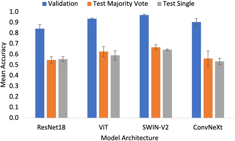 | ||
| Fig. 5 Mean accuracy metrics across 3 independent trials for the validation and test sets (majority vote and single) for the ResNet18, ViT, SWIN-V2 and ConvNeXt architectures. Split factor, n = 10 for all cases. | ||
The trend in performance can be explained by consideration of the network design. The sliding window in convolutional neural networks is an effective tool for localised feature extraction. However, the design experiences limitations with respect to modelling longer-range dependencies as they have limited receptive fields.37 This is pertinent to the flowability application when considering the aim is to predict a bulk property. Unlike other computer vision tasks, where localised features can be important (for example the shape of flower petals or particular facial features), in this work, we must consider the sample in its entirety. This is because a bulk property results from the material as a whole rather than features which correspond to particular, individual particles. It is possible to increase the size of the receptive field in convolutional networks by making the convolutional sliding window larger. However, it has been shown that attention is a superior approach.38 Attention models are better able to model long-term dependencies without incurring the computational cost of larger convolutional sliding windows, and so it follows that they show better performance in flowability prediction.
Having established the SWIN-V2 model offers superior performance, a comprehensive split factor evaluation was performed with the resizing applied. The purpose of this experiment was to assess how the model's performance changed when it was trained having seen a smaller sample of the bulk powder. During the splitting evaluation in Section 3.2, the experiment assessed if the input size of the image is limiting, but the model eventually sees the entirety of the raw Morphologi G3 image, just in different-sized crops. In this case, by applying both splitting and cropping, different amounts of the Morphologi G3 image get entirely removed. This further challenges the assumption that we can predict bulk properties from images containing only small samples of the bulk material.
Fig. 6 shows that performance increases up to n = 7, and then begins to drop when n > 7. This suggests that beyond n = 7, there is no further gain from capturing more pixels in the input images. Intuitively, capturing more of the Morphologi G3 image gives the network more information and hence it can better capture the relationship. The authors suggest this result arises because there is no additional particle detail. In other words, the model had already seen all the different particle features of the sample. As a result, when shown more of the same information, the system becomes prone to overfitting and so the performance drops. This is the same observation seen when excessive image augmentation is used as part of the preprocessing pipelines in computer vision tasks. It should be noted that this result could also be influenced by the overall dataset size. As such, extensions of this project which aim to compile a larger dataset must investigate the full range of possible n values, as with more information the risk of overfitting is reduced.
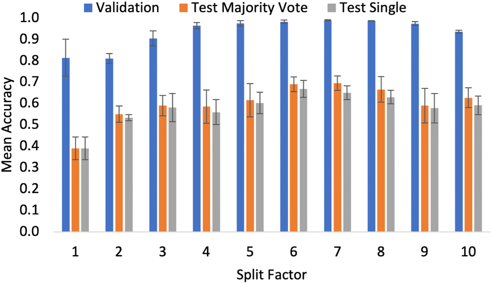 | ||
| Fig. 6 Accuracy metrics for the SWIN-V2 model across the entire range of split factor (n) values. | ||
3.4 External testing
To better understand the model's decision-making process, Fig. 7 shows a confusion matrix which presents the sum of the prediction across the five k-fold splits for the external test sets. Such evaluation ensures there is no overfitting to the training or validation set, but also represents a typical deployment scenario for the trained model.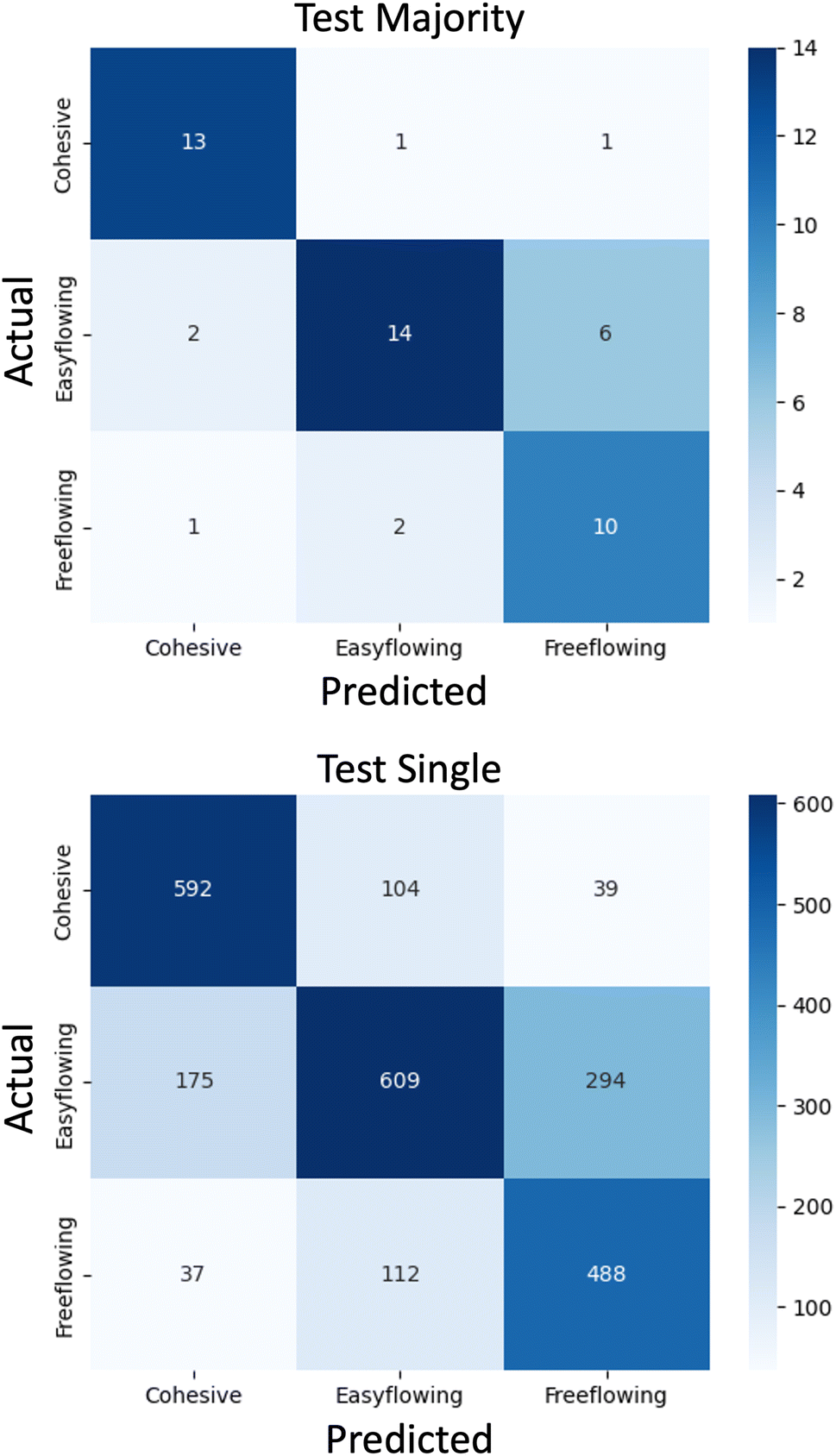 | ||
| Fig. 7 Confusion matrices showing the distribution of prediction outcomes on the external test set using the SWIN-V2 model. Displayed for majority vote (top) and single (bottom) evaluation approaches. Plots were taken from a single trial where split factor n = 7. | ||
All of the results in this section correspond to the best single trial of the n = 7 SWIN-V2 model, which was the one showcasing the best mean accuracy metrics during architecture testing. As such, the accuracy metrics shown in Table 2 differ from the mean across the three trials. The accuracy values for this trial were 0.740 and 0.689 for the single and majority vote, respectively. When considering the external test set was comprised of 9 samples in each fold, these accuracy metrics correspond to ultimately predicting an average of 6 or 7 correctly out of the possible 9 samples during each k-fold split. Although the evaluation here used a limited number of examples; the results suggest that the predictions of unseen flowability can be made with reasonable accuracy, and the k-fold testing ensures this metric is representative, reproducible and not arising due to favourable sample splitting.
| Class | Accuracy single | Accuracy majority vote |
|---|---|---|
| Cohesive | 0.805 | 0.867 |
| Easy flowing | 0.565 | 0.636 |
| Free flowing | 0.766 | 0.769 |
| Overall | 0.689 | 0.740 |
Table 2 shows the accuracy metrics on a per-class basis from the trial presented in the confusion matrix. From this, it was clear that the model was better at predicting each of the extremity classes (cohesive and free-flowing) compared to the middle, easy-flowing class. Making this comparison also demonstrates that the majority vote system should be used as standard practice, as in every case it had better accuracy than the single system. The authors note that the single system's primary purpose in this evaluation was to provide better interpretability, as individual mistakes do not cause such large accuracy drops when the number of test samples was much higher. However, the difference in accuracy between the single and majority vote systems was small, which shows that there are only a small number of crops from each raw Morphologi G3 image that get assigned labels that differ from the majority consensus. This is shown by the confusion matrices in Fig. 7, as the trends in distribution predictions (shown by the shades of blue colouring) are similar.
3.5 Manufacturing considerations
The misclassification of a cohesive material as free-flowing can result in wasted resources and time since this material would be wrongly considered suitable for direct compression.39 In this scenario, additional steps such as granulation, incorporation of additives, or transitioning to continuous processes must be used which incur additional costs with respect to time, energy and materials. As such, from a deployment perspective, this mistake carries more negative impact than other misclassifications when predicting flowability. Despite this, powder flow is one of many considerations that are part of the pharmaceutical development process, and it is important to consider all these factors must be tolerable to avoid halting the development of a specific product. As shown in Fig. 7, when examples are misclassified, there were always fewer predicted as cohesive compared to the other incorrect class. Given one of the primary advantages of using DL for this task was to minimise wasted resources, this represents the most favoured, least damaging scenario for when the wrong predictions are made. Furthermore, the opportunity to predict the flowability of materials at the milligram scale is valuable as the amount of material is much lower than that needed for reliable experimental flow characterization.4 Conclusions
In this work, we present a data-driven approach to predicting powder flowability from images of the constituent particles. To do so, DL for image classification was leveraged using a transfer learning approach. We evaluate four state-of-the-art network architectures from literature which showed attention-based models offer superior performance in flowability prediction. In particular, the SWIN-V2 model offered the best performance, with mean classification accuracy values of 0.989 ± 0.003 and 0.695 ± 0.034 for the validation and external test sets respectively. The model was evaluated using a stratified cross-validation approach and repeat trials to ensure representative, accurate metrics were recorded. We further investigated the effect of reducing image size when training neural models to assess if the entirety of a bulk sample was necessary to predict powder flow. The authors note that assessing this method against literature benchmarks with equal datasets was not possible at the time of writing. Such analysis forms a key area of future work that will be investigated. This work was developed to overcome the challenges associated with characterizing particle flow. Experimental flowability measurement procedures require large quantities of samples, lengthy measurement times and experiences difficulty in recording reproducible results. Using a predictive model offers the ability to overcome these development obstacles. The presented approach requires significantly less material than is needed for laboratory flowability measurements. This reduction in materials not only reduces development costs associated with synthesising sufficient quantities but further reduces the need for repeated testing which is time-consuming. Overall, these advantages can help improve the efficiency of overcoming flowability challenges during pharmaceutical manufacturing which will also aid in creating more sustainable manufacturing practices that are less resource intensive.Appendices
A List of materials
| Material | Supplier |
|---|---|
| 1-Octadecanol | Sigma-Aldrich |
| 4-Aminobenzoic acid | Sigma-Aldrich |
| Ac-Di-Sol | Dupont |
| Affinisol | Dupont |
| Cetyl alcohol | Sigma-Aldrich |
| Avicel PH-101 | Dupont |
| Azelaic acid | Sigma-Aldrich |
| Benecel K100M | Dupont |
| Caffeine | Sigma-Aldrich |
| Calcium carbonate | Sigma-Aldrich |
| Calcium phosphate dibasic | Sigma-Aldrich |
| Cellulose | Sigma-Aldrich |
| Cholic acid | Sigma-Aldrich |
| D-Glucose | Sigma-Aldrich |
| Dimethyl fumarate | Sigma-Aldrich |
| D-Sorbitol | Sigma-Aldrich |
| FastFlo 316 | Dupont |
| Granulac 230 | Meggle Pharma |
| HPMC | Sigma-Aldrich |
| Ibuprofen 50 | BASF |
| Ibuprofen 70 | Sigma-Aldrich |
| Lidocaine | Sigma-Aldrich |
| Lubritose mannitol | Kerry |
| Lubritose MCC | Kerry |
| Lubritose PB | Kerry |
| Magnesium stearate | Roquette |
| Magnesium stearate | Sigma-Aldrich |
| Mefenamic acid | Sigma-Aldrich |
| Methocel DC2 | Colorcon |
| Microcel MC-200 | Roquette |
| Mowiol 18-88 | Sigma-Aldrich |
| Paracetamol granular special | Sigma-Aldrich |
| Paracetamol powder | Sigma-Aldrich |
| Parteck 50 | Sigma-Aldrich |
| Pearlitol 100SD | Roquette |
| Pearlitol 200SD | Roquette |
| Phenylephedrine | Sigma-Aldrich |
| Pluronic F-127 | Sigma-Aldrich |
| Potassium chloride | Sigma-Aldrich |
| PVP | Sigma-Aldrich |
| S-Carboxymethyl-L-cysteine | Sigma-Aldrich |
| Sodium stearyl fumarate | Sigma-Aldrich |
| Soluplus | BASF |
| Span 60 | Sigma-Aldrich |
| Stearyl alcohol | Sigma-Aldrich |
B List of flow function coefficients for all unique single and multi-component materials
| Material | FFc | Class |
|---|---|---|
| 1-Octadecanol | 2.26 | Cohesive |
| 4-Aminobenzoic acid | 5.03 | Easy flowing |
| Ac-Di-Sol SD | 14.32 | Free flowing |
| Affinisol HPMC | 8.11 | Easy flowing |
| Avicel PH-101 | 7.46 | Easy flowing |
| Azelaic acid | 2.10 | Cohesive |
| Benecel K100M | 28.94 | Free flowing |
| Caffeine | 3.55 | Cohesive |
| Calcium carbonate (20%) – binary | 4.66 | Easy flowing |
| Calcium carbonate (20%) – multicomponent | 8.11 | Easy flowing |
| Calcium carbonate (40%) – binary | 2.13 | Cohesive |
| Calcium carbonate (40%) – multicomponent | 3.16 | Cohesive |
| Calcium carbonate (5%) – binary | 24.25 | Free flowing |
| Calcium carbonate (5%) – multicomponent | 42.37 | Free flowing |
| Calcium carbonate | 4.00 | Easy flowing |
| Calcium phosphate dibasic | 2.97 | Cohesive |
| Cellulose | 3.32 | Cohesive |
| Cetyl alcohol | 1.86 | Cohesive |
| Cholic acid | 3.58 | Cohesive |
| D-Glucose | 9.29 | Easy flowing |
| D-Sorbitol | 14.74 | Free flowing |
| Dimethyl fumarate | 13.02 | Free flowing |
| FastFlo 316 | 49.19 | Free flowing |
| Granulac 230 | 3.22 | Cohesive |
| HPMC | 17.98 | Free flowing |
| Ibuprofen (20%) + FastFlo 316 | 23.00 | Free flowing |
| Ibuprofen 50 | 7.42 | Easy flowing |
| Ibuprofen 50 (20%) – binary | 36.25 | Free flowing |
| Ibuprofen 50 (40%) – binary | 19.66 | Free flowing |
| Ibuprofen 50 (5%) – binary | 26.53 | Free flowing |
| Ibuprofen 50 (5%) – multicomponent | 50.91 | Free flowing |
| Ibuprofen 70 | 9.58 | Easy flowing |
| Lidocaine | 2.33 | Cohesive |
| Lubritose mannitol | 30.00 | Free flowing |
| Lubritose MCC | 35.23 | Free flowing |
| Lubritose PB | 28.84 | Free flowing |
| Magnesium stearate | 4.02 | Easy flowing |
| Mefenamic acid | 12.07 | Free flowing |
| Mefenamic acid (20%) – multicomponent | 21.35 | Free flowing |
| Mefenamic acid (35%) – binary | 22.62 | Free flowing |
| Mefenamic acid (35%) – multicomponent | 24.53 | Free flowing |
| Mefenamic acid (5%) – binary | 25.02 | Free flowing |
| Mefenamic acid (5%) – multicomponent | 31.22 | Free flowing |
| Methocel DC2 | 10.37 | Free flowing |
| Microcel MC-102 | 16.80 | Free flowing |
| Microcel MC-200 | 4.46 | Easy flowing |
| Mowiol 18-88 | 3.78 | Cohesive |
| Paracetamol granular special | 12.94 | Free flowing |
| Paracetamol granular special (20%) – binary | 15.90 | Free flowing |
| Paracetamol granular special (20%) – multicomponent | 5.05 | Easy flowing |
| Paracetamol granular special (40%) – binary | 12.50 | Free flowing |
| Paracetamol granular special (40%) – multicomponent | 35.29 | Free flowing |
| Paracetamol granular special (5%) – binary | 20.22 | Free flowing |
| Paracetamol powder | 3.88 | Cohesive |
| Paracetamol powder(20%) – binary | 7.72 | Easy flowing |
| Paracetamol powder(20%) – multicomponent | 9.55 | Easy flowing |
| Paracetamol powder(40%) – binary | 4.53 | Easy flowing |
| Paracetamol powder(40%) – multicomponent | 6.53 | Easy flowing |
| Paracetamol powder(5%) – binary | 14.67 | Free flowing |
| Parteck 50 | 1.16 | Cohesive |
| Pearlitol 100SD | 38.21 | Free flowing |
| Pearlitol 200SD | 20.92 | Free flowing |
| Pearlitol 300 DC | 27.00 | Free flowing |
| Phenylephrine | 5.02 | Easy flowing |
| Pluronic F-127 | 10.07 | Free flowing |
| Potasium chloride | 3.35 | Cohesive |
| PVP | 14.78 | Free flowing |
| S-Carboxymethyl-L-cysteine | 4.42 | Easy flowing |
| Sodium stearyl fumarate | 5.60 | Easy flowing |
| Soluplus | 8.47 | Easy flowing |
| Span 60 | 1.90 | Cohesive |
| Stearyl alcohol | 2.72 | Cohesive |
C Table of metrics for ResNet18 split factors
| Split factor | Validation | Test single | Test majority | |||
|---|---|---|---|---|---|---|
| Mean accuracy | StDev | Mean accuracy | StDev | Mean accuracy | StDev | |
| 2 | 0.846 | 0.049 | 0.592 | 0.058 | 0.600 | 0.040 |
| 4 | 0.868 | 0.014 | 0.537 | 0.008 | 0.527 | 0.031 |
| 6 | 0.788 | 0.005 | 0.557 | 0.016 | 0.560 | 0.035 |
| 8 | 0.848 | 0.007 | 0.535 | 0.049 | 0.527 | 0.046 |
| 10 | 0.780 | 0.039 | 0.579 | 0.042 | 0.580 | 0.053 |
D Table of metrics for architecture testing
| Model | Validation | Test single | Test majority | |||
|---|---|---|---|---|---|---|
| Mean accuracy | StDev | Mean accuracy | StDev | Mean accuracy | StDev | |
| ResNet18 | 0.842 | 0.037 | 0.554 | 0.024 | 0.547 | 0.031 |
| ViT | 0.935 | 0.007 | 0.591 | 0.043 | 0.627 | 0.046 |
| SwinV2 | 0.970 | 0.009 | 0.643 | 0.007 | 0.667 | 0.023 |
| ConvNeXt | 0.905 | 0.032 | 0.534 | 0.029 | 0.560 | 0.072 |
E Table of metrics for SWIN-V2 split factors
| Split factor | Validation | Test single | Test majority | |||
|---|---|---|---|---|---|---|
| Mean accuracy | StDev | Mean accuracy | StDev | Mean accuracy | StDev | |
| 1 | 0.813 | 0.086 | 0.390 | 0.053 | 0.390 | 0.053 |
| 2 | 0.810 | 0.023 | 0.534 | 0.014 | 0.550 | 0.038 |
| 3 | 0.904 | 0.035 | 0.581 | 0.065 | 0.590 | 0.048 |
| 4 | 0.964 | 0.014 | 0.559 | 0.058 | 0.585 | 0.077 |
| 5 | 0.974 | 0.013 | 0.602 | 0.050 | 0.615 | 0.077 |
| 6 | 0.982 | 0.007 | 0.668 | 0.040 | 0.690 | 0.035 |
| 7 | 0.989 | 0.003 | 0.650 | 0.032 | 0.695 | 0.034 |
| 8 | 0.987 | 0.001 | 0.629 | 0.031 | 0.665 | 0.060 |
| 9 | 0.973 | 0.009 | 0.578 | 0.068 | 0.590 | 0.081 |
| 10 | 0.935 | 0.007 | 0.591 | 0.043 | 0.627 | 0.046 |
F Class confidence scores of the external test set
| Ground truth label | Predicted label | Material name | Easy flowing | Free flowing | Cohesive |
|---|---|---|---|---|---|
| Cohesive | Easy flowing | Calcium phosphate dibasic | 0.9776 | 0.000595 | 0.02181 |
| Cohesive | Free flowing | Mowiol 18-88 | 0.00025454 | 0.97428 | 0.025462 |
| Easy flowing | Cohesive | Calcium carbonate (20%) – multicomponent | 0.0088 | 0.0041 | 0.9871 |
| Easy flowing | Free flowing | Microcel MC-200 | 0.0012781 | 0.99872 | 6.233E-06 |
| Free flowing | Easy flowing | Calcium carbonate (5%) – multicomponent | 0.51524 | 0.4845 | 0.00025947 |
| Free flowing | Cohesive | Ac-Di-Sol | 0.2618 | 0.0092 | 0.7291 |
Data availability
The source code and experimental data for this project is available at https://github.com/MRW-Code/cmac_particle_flow.Author contributions
Conceptualization was a collaborative effort between M. R. W, L. P. D and A. D. V. All laboratory measurements were carried out by L. P. D. The source code for the project was developed by M. R. W. Computational experimentation was designed collaboratively between M. R. W, L. P. D, J. A and A. D. V, with testing carried out by M. R. W and J. A. The computational results were finalized and collated for inclusion in the manuscript by M. R. W. Writing of the manuscript was led with an equal contribution between M. R. W and L. P. D, with all authors providing critical feedback. B. C. D was responsible for the PhD funding to support M. R. W, and C. J. B and A. J. F for the funding to support L. P. D.Conflicts of interest
There are no conflicts to declare.Acknowledgements
The authors thank EPSRC and the EPSRC Future Continuous Manufacturing and Advanced Crystallization Research Hub (Grant Ref. EP/P006965/1) for funding this work. The authors acknowledge that parts of this work were carried out in the CMAC National Facility supported by a UK Research Partnership Fund (UKRPIF) award from the Higher Education Funding Council for England (HEFCE) (Grant Ref. HH13054). M. R. W thanks the PhD studentship funded by CMAC Future Manufacturing Research Hub and the Centre for Sustainable and Circular Technologies at the University of Bath. All the authors thank Dr Tom Fincham Haines and the Department of Computer Science at the University of Bath for their support in accessing the hardware resources needed for this work.References
- A.-P. Karttunen, H. Wikström, P. Tajarobi, M. Fransson, A. Sparén, M. Marucci, J. Ketolainen, S. Folestad, O. Korhonen and S. Abrahmsén-Alami, Eur. J. Pharm. Sci., 2019, 133, 40–53 CrossRef CAS PubMed.
- S. Lakio, T. Ervasti, P. Tajarobi, H. Wikström, M. Fransson, A.-P. Karttunen, J. Ketolainen, S. Folestad, S. Abrahmsén-Alami and O. Korhonen, Eur. J. Pharm. Sci., 2017, 109, 514–524 CrossRef CAS PubMed.
- W. J. Roth, A. Almaya, T. T. Kramer and J. D. Hofer, J. Pharm. Sci., 2017, 106, 1339–1346 CrossRef CAS PubMed.
- J. Li and Y. Wu, Lubricants, 2014, 2, 21–43 CrossRef.
- Y. Endo and M. Alonso, Chem. Eng. Res. Des., 2002, 80, 625–630 CrossRef CAS.
- A. Crouter and L. Briens, AAPS PharmSciTech, 2014, 15, 65–74 CrossRef CAS PubMed.
- S. C. Gad, Pharmaceutical manufacturing handbook: production and processes, John Wiley & Sons, 2008 Search PubMed.
- J. Prescott and R. A. Barnum, Pharm. Technol., 2000, 24, 60–84 CAS.
- H. Abe, S. Yasui, A. Kuwata and H. Takeuchi, Chem. Pharm. Bull., 2009, 57, 647–652 CrossRef CAS PubMed.
- J. Schwedes, Granul. Matter, 2003, 5, 1–43 CrossRef.
- S. Koynov and F. J. Muzzio, A quantitative approach to understand raw material variability, Process Simulation and Data Modeling in Solid Oral Drug Development and Manufacture, Springer, New York, 2016, pp. 85–104 Search PubMed.
- N. Sandler, K. Reiche, J. Heinämäki and J. Yliruusi, Pharmaceutics, 2010, 2, 275–290 CrossRef CAS PubMed.
- G. Tan, D. A. V. Morton and I. Larson, Curr. Pharm. Des., 2015, 21, 5751–5765 CrossRef CAS PubMed.
- S. Divya and G. Ganesh, J. Pharm. Sci., 2019, 11, 25–29 CAS.
- J. S. Kaerger, S. Edge and R. Price, Eur. J. Pharm. Sci., 2004, 22, 173–179 CrossRef CAS PubMed.
- L. Liu, I. Marziano, A. Bentham, J. Litster, E. White and T. Howes, Int. J. Pharm., 2008, 362, 109–117 CrossRef CAS PubMed.
- W. Yu, K. Muteki, L. Zhang and G. Kim, J. Pharm. Sci., 2011, 100, 284–293 CrossRef CAS PubMed.
- H. Barjat, S. Checkley, T. Chitu, N. Dawson, A. Farshchi, A. Ferreira, J. Gamble, M. Leane, A. Mitchell, C. Morris, K. Pitt, R. Storey, F. Tahir and M. Tobyn, J. Pharm. Innov., 2021, 16, 181–196 CrossRef.
- A. W. Jenike, Storage and flow of solids, Bulletin No. 123, 1964, vol. 53, p. 26 Search PubMed.
- S. Almeida-Prieto, J. Blanco-Méndez and F. J. Otero-Espinar, J. Pharm. Sci., 2006, 95, 348–357 CrossRef CAS PubMed.
- M.-N. Pons, H. Vivier, V. Delcour, J.-R. Authelin and L. Paillères-Hubert, Powder Technol., 2002, 128, 276–286 CrossRef CAS.
- J. Howard and S. Gugger, Information, 2020, 11, 108 CrossRef.
- R. Wightman, PyTorch Image Models, 2019, https://github.com/rwightman/pytorch-image-models Search PubMed.
- C. Khosla and B. S. Saini, International Conference on Intelligent Engineering and Management, ICIEM, 2020, pp. 79–85 Search PubMed.
- J. Wang, L. Perezet al., Convolutional Neural Networks for Visual Recognition, 2017, 11, pp. 1–8 Search PubMed.
- C. Shorten and T. M. Khoshgoftaar, J. Big Data, 2019, 6, 60 CrossRef.
- K. He, X. Zhang, S. Ren and J. Sun, Proceedings of the IEEE conference on computer vision and pattern recognition, 2016, pp. 770–778 Search PubMed.
- A. Dosovitskiy, L. Beyer, A. Kolesnikov, D. Weissenborn, X. Zhai, T. Unterthiner, M. Dehghani, M. Minderer, G. Heigold, S. Gelly, J. Uszkoreit and N. Houlsby, An Image is Worth 16 × 16 Words: Transformers for Image Recognition at Scale, arXiv, 2021, preprint, arXiv:2010.11929.
- Z. Liu, Y. Lin, Y. Cao, H. Hu, Y. Wei, Z. Zhang, S. Lin and B. Guo, Proceedings of the IEEE/CVF International Conference on Computer Vision, ICCV, 2021 Search PubMed.
- Z. Liu, H. Hu, Y. Lin, Z. Yao, Z. Xie, Y. Wei, J. Ning, Y. Cao, Z. Zhang, L. Dong, F. Wei and B. Guo, International Conference on Computer Vision and Pattern Recognition, CVPR, 2022 Search PubMed.
- Z. Liu, H. Mao, C.-Y. Wu, C. Feichtenhofer, T. Darrell and S. Xie, Proceedings of the IEEE/CVF Conference on Computer Vision and Pattern Recognition, CVPR, 2022 Search PubMed.
- A. Paszke, S. Gross, F. Massa, A. Lerer, J. Bradbury, G. Chanan, T. Killeen, Z. Lin, N. Gimelshein, L. Antiga, A. Desmaison, A. Kopf, E. Yang, Z. DeVito, M. Raison, A. Tejani, S. Chilamkurthy, B. Steiner, L. Fang, J. Bai and S. Chintala, Advances in Neural Information Processing Systems, Curran Associates, Inc., 2019, vol. 32, pp. 8024–8035 Search PubMed.
- O. Russakovsky, J. Deng, H. Su, J. Krause, S. Satheesh, S. Ma, Z. Huang, A. Karpathy, A. Khosla and M. Bernstein, Int. J. Comput. Vis., 2015, 115, 211–252 CrossRef.
- F. Pedregosa, G. Varoquaux, A. Gramfort, V. Michel, B. Thirion, O. Grisel, M. Blondel, P. Prettenhofer, R. Weiss, V. Dubourg, J. Vanderplas, A. Passos, D. Cournapeau, M. Brucher, M. Perrot and E. Duchesnay, J. Mach. Learn. Technol., 2011, 12, 2825–2830 Search PubMed.
- H. G. Brittain, Pharm. Technol., 2002, 26(7), 67–73 Search PubMed.
- A. P. Steiner, A. Kolesnikov, X. Zhai, R. Wightman, J. Uszkoreit and L. Beyer, J. Mach. Learn. Res., 2022, 2835–8856 Search PubMed.
- Y. Wu, Y. Ma, J. Liu, J. Du and L. Xing, Inf. Sci., 2019, 490, 317–328 CrossRef PubMed.
- N. Parmar, A. Vaswani, J. Uszkoreit, L. Kaiser, N. Shazeer, A. Ku and D. Tran, International Conference on Machine Learning, 2018, pp. 4055–4064 Search PubMed.
- M. Leane, K. Pitt, G. Reynolds and M. C. S. W. Group, Pharm. Dev. Technol., 2015, 20, 12–21 CrossRef CAS PubMed.
| This journal is © The Royal Society of Chemistry 2023 |