Extrapolation performance improvement by quantum chemical calculations for machine-learning-based predictions of flow-synthesized binary copolymers

Abstract

The properties of polymers are highly dependent on the combination and composition ratio of the monomers used to prepare them; however, the large number of available monomers makes an exhaustive investigation of all the possible combinations difficult. In the present study, five binary copolymers were prepared by radical polymerization using a flow reactor and the prediction performance of a machine learning model constructed using the obtained data was evaluated for the interpolation and extrapolation regions. Copolymer analysis was performed using ultra-high-performance liquid chromatography, and the measurement results were analysed to calculate the monomer conversion and monomer composition ratio in the polymer, which were used as objective variables. A prediction model was constructed using the process variables during polymerization and additional molecular descriptors (i.e., molecular flags (one-hot encoding), fingerprints or quantum chemical calculation values) related to the monomer type as explanatory variables. In the interpolated regions where all monomer types used were included in the training data, the prediction accuracy was high irrespective of the molecular descriptors added to the process variables. In the extrapolation region, the model that included explanatory variables corresponding to quantum chemical calculation values representing the energy generated when radical reactions occur, showed a high prediction accuracy for each objective variable. We found that quantum chemical calculation values (especially the molecular orbital energy of monomers in the extrapolation region) are important factors in the search for new binary copolymers prepared by radical polymerization. The proposed model is expected to accelerate the development of polymers using new monomers.

---

Introduction

For polymer materials, the monomer type and composition ratios are important factors that directly affect basic performance characteristics such as mechanical, thermal and flow properties. Polymethyl methacrylate (PMMA), a representative polymer material, is used in a wide range of applications such as automotive parts, lighting fixtures and building materials, because of its excellent transparency and weather resistance. Methyl methacrylate (MMA) has long been investigated not only as a homopolymer but also as a copolymer. Copolymerization with monomers such as styrene (St)^1–4 and glycidyl methacrylate (GMA)^5–7 has been investigated from viewpoints such as reactivity ratio, molecular weight, sequencing, and thermal properties. However, the copolymers reported thus far are only a fraction of the myriad possible combinations. Because exhaustively studying all of the possible copolymers is inefficient and impractical, material exploration using machine learning (ML) has attracted much attention.

Materials exploration using ML has been investigated for a wide range of purposes, including searching for polymer compositions that exhibit required properties,^8–10 classifying polymers by their crystalline phase and microstructure,^11,12 and predicting the physical properties of polymers.¹³ As summarized by Hu et al., the number of different algorithms and learning models is increasing at an accelerating rate and, with it, the scope of exploration.¹⁴ ML can be conducted with a small amount of data; however, many data are preferable considering the scope of the material search and the desired prediction accuracy. Therefore, a high-throughput reactor is one of the critical elements for more efficient studies using ML. Material exploration^15–17 and analysis^18–20 using high-throughput instruments, whether in organic or inorganic chemistry, are already being actively studied in combination with ML. Coley et al., for example, used ML to predict the synthetic pathways for organic compounds, created a platform for their synthesis using a robotic flow device and demonstrated the platform's efficacy for 15 drugs or drug analogues.²¹ In addition, reactors in polymer synthesis are becoming increasingly high-throughput. Polymers have been used only in limited cases, such as applications that require photoreactive polymers,²² because they contain certain components produced by heterogeneity, introducing a risk of blocking the piping because of large viscosity changes during polymerization.

In recent years, microchemical approaches in the polymer field have been developed and polymerization by flow synthesis using a micromixer has been investigated.²³ Flow synthesis is being actively studied in combination with ML, not only because it enables easy control of polymers and produces polymers with narrow molecular-weight distributions but also because it is highly efficient in production, enabling the collection of large amounts of data.^24,25 Reis et al. synthesized copolymers using any combination of six monomers by radical polymerization in flow reactors.²⁶ By incorporating ML methods, they identified more than 10 copolymer compositions that are superior to conventional materials within a search range representing less than 0.9% of the total composition space. Tan et al. used an in-line analyser to continuously acquire time-dependent analytical data, enabling the prediction of polystyrene conversion and molecular-weight distribution charts.²⁷ Their results clearly show that the combination of ML and flow polymerization can be used to study polymers more efficiently. However, predicting polymerization using monomers not included in the learning process (extrapolated regions), which is highly desirable in the search for new materials makes it difficult to achieve high accuracy.

We have constructed a flow copolymerization system using a microflow mixer and are investigating copolymerization with more equal composition ratios for MMA–St and MMA–GMA copolymers.²⁸ In the present work, we synthesized binary copolymers of MMA and GMA/St/4-acetoxystyrene (PACS)/tetrahydrofurfuryl methacrylate (THFMA)/cyclohexyl methacrylate (CHMA) via a free-radical method using the same flow copolymerization system used in our previous work. To more efficiently develop new materials, we used ML predictions to explore the extrapolation region for monomers that would provide desirable polymer properties.

Experimental methods

Polymer synthesis and characterization

Five binary copolymers were synthesized using six different monomers (Fig. 1): MMA, GMA, St, PACS, THFMA and CHMA. Herein, GMA, St, PACS, THFMA and CHMA are classified as M1 and MMA as M2 because the copolymerization reaction is performed by combining MMA with the five other monomers. Each copolymer was synthesized by radical polymerization using the manual flow reactor shown in Fig. 2 under various process conditions (M1 ratio, M2 ratio, initiator ratio, S/M ratio, flow rate and reaction temperature). Herein, the S/M ratio is the ratio between the solvent (S) and monomer (M). Bottle-1 and bottle-2 were prepared with the same S/M ratio. For the initiator, 2,2′-azobis(2,4-dimethylvaleronitrile) was selected because its thermal decomposition rate can be easily controlled in a water bath, and for the solvent, 1-methoxy-2-propanol was employed because it is an effective solvent for many monomers and it has a high boiling point. The reason for choosing flow synthesis as the polymerization method is explained in detail in the discussion for Examination 0. The copolymers were analysed using ultra-high-performance liquid chromatography (UHPLC) to calculate the M1 conversion (M1_conv.), M2 conversion (M2_conv.) and M1 composition ratio (M1_CR) in polymers. The M1_conv., M2_conv. and M1_CR in polymers were calculated using the following equations:where R₀ is the mass fraction of each monomer at a reaction time of 0 min (no reaction), R_t is the mass fraction of each monomer at reaction time t, and M1_fr and M2_fr are the composition ratio of each monomer used in the preparation. A total of 247 copolymers were synthesized and used as the dataset for ML. Details of the experimental and analytical conditions are provided in the ESI.†

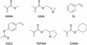Fig. 1 Chemical structures of monomers used in present work: GMA, St, PACS, THFMA and CHMA are classified as M1 and MMA as M2.

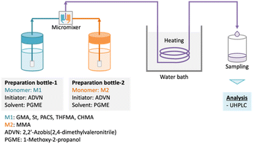Fig. 2 Model of flow synthesis reactor. Two bottles containing each monomer, initiator, and solvent are mixed using a micromixer, and synthesis is performed at the required temperature.

Validation

A training–test split was conducted using the 247 copolymers synthesized as shown in Fig. 3 to verify the two types of examination described below. Examination 1 consisted of double cross validation to include copolymers with the same type of monomer for both the training and test data to obtain predictions for combinations of existing monomers (interpolated regions). In this case, validation was applied tenfold on both the outer and the inner loop (training data : test data = 9 : 1). In Examination 2, molecular extrapolation validation was conducted with four copolymers as training data and the remaining copolymer as test data to obtain predictions for combinations with new monomers (extrapolation region). The number of data used for training depends on the monomer type (number of training data: 175–219).

Fig. 3 Model of validation method. Examination 1 involves copolymers with the same type of monomer for the training and test data. Examination 2 uses four copolymers for training data and the remaining copolymer for test data.

ML algorithms

For the two aforementioned training–test split datasets, we used ν-support vector regression (ν-SVR),²⁹ random forest (RF) and partial least-squares regression (PLS) to construct models to predict the M1_conv., M2_conv., M1_CR and the calculated M1_CR (C_M1_CR). Herein, C_M1_CR is the M1_CR calculated using the predictions of M1_conv. and M2_conv. The hyperparameters for each model were optimized using the Optuna optimization software framework.³⁰

Explanatory variables

For both validation methods, four explanatory variables were used, feature sets A–D. Feature set A represents process variables (M1 ratio, initiator ratio, S/M ratio, reaction temperature and reaction time), and feature sets B–D comprise molecular flags (one-hot encoding), fingerprints (RDKit: 208 features)³¹ and calculated quantum chemical values (36 features), respectively. The above information is summarized in Fig. 4.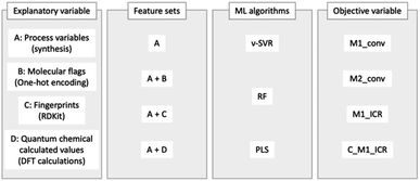

Fig. 4 Overview of methods: explanatory variables, feature sets, ML algorithms, and objective variables.

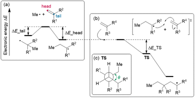
Feature set D is composed of the parameters calculated by density functional theory (DFT), consisting of (D-1) two reaction energies, (D-2) nine activation energies, (D-3) nine geometrical parameters, and (D-4) 16 orbital energies. Focusing on the polymerization of MMA and monomer X (X = GMA, ST, CHMA, THFMA, PACS), we note that the reaction starts from the attack of the radical initiator to the monomer (MMA or X), affording an MMA radical or X radical (denoted as MMA* or X*, respectively). Thus, the reaction energies for head- and tail-attack of the methyl radical (the model radical initiator) and monomer X (Fig. 5(a)) were used for feature set D-1. (Note that the attack to MMA was excluded from the feature set because it was commonly included in all our target reactions.) The second stage of polymerization is C–C bond formation between a monomer and a radical (Fig. 5(b)), such as (i) MMA and X*, (ii) X and MMA*, (iii) X and X* and (iv) MMA and MMA*. Because the transition state (TS) of C–C bond formation has three staggered conformations, each reaction could have three stable TS structures. Thus, the energy difference between the TS with three staggered conformations and the dissociation limit (radical + monomer) for reactions (i), (ii) and (iii) were used for feature set D-2, and the dihedral angles around the reactive C atoms at these TSs (Fig. 5(c)) were used for feature set D-3. We also gathered the features set D-4, i.e., the orbital energies of the highest occupied molecular orbital (HOMO) and lowest unoccupied molecular orbital (LUMO) for X, those of the singly occupied molecular orbital (SOMO) and LUMO for X* and the HOMO–SOMO and SOMO–LUMO energy gaps between monomer A and radical B*, where (A, B*) are (MMA, X*), (X, MMA*) and (X, X*).

Fig. 5 Overview of DFT Calculations. (a) Feature sets D related to the reaction energies of the head- and tail-attack of the methyl radical to the monomer (ΔE_head and ΔE_tail, respectively), (b) the relative energy of the TS from the isolated radical and the monomer (ΔE_TS) and (c) the dihedral angle θ for the TS geometry.

The calculation scheme for the 36 aforementioned features was as follows: first, the monomer conformers were generated from the Simplified Molecular-Input Line-Entry System (SMILES) using the RDKit cheminformatics software. As many as five conformers with large structural differences were then extracted for further geometrical optimization at the xTB level of theory. Second, the geometries of the model radicals (i.e. the products of monomers and methyl radicals) were calculated using an automated reaction-path search method known as the artificial force-induced reaction (AFIR) method at the xTB level of theory. To gather the conformers of the head- and tail-type model radicals, we randomly selected the monomer conformers and applied the AFIR calculation by adding the artificial force between the head or tail C atom of the monomer and the C atom of the methyl radical. This calculation was continued until the last three AFIR calculations did not find a new product. Third, to gather the TSs between the monomer and head-type model radical, we applied the AFIR method by adding the force between the reactive C atoms (i.e., the head C atom of the monomer and the tail C atom of the model radical). All the appropriate local minima and maxima (whose reactive C–C bond length was 2.20–3.24 Å) along the AFIR reaction pathways were reoptimized without any restriction at the B3LYP-D3/def2-SVP level of theory. On the basis of the obtained TS structures, we prepared three staggered conformations by modifying the dihedral angle around the reactive C atoms and then reoptimizing them. The geometry optimization and AFIR calculations were conducted using the Global Reaction Route Mapping (GRRM) program with the energies and energy derivatives computed by the Gaussian 16 program (for the DFT level) and the ORCA program (for the xTB level).

Results and discussion

Examination 0 (comparison of batch polymerization and flow polymerization)

This section explains why flow polymerization was chosen for the present study. Polymer synthesis using a flow reactor is expected to lead to a large amount of experimental data and is considered a highly effective method for ML. However, even if a large amount of experimental data are obtained, using a flow reactor is hardly useful if the learning model constructed using the data is inaccurate. A polymerization method that can make more accurate predictions must be selected. Therefore, we compared the prediction accuracy between flow synthesis and batch synthesis for M1_conv. (Fig. 6). For both polymerization methods, validation was conducted using ν-SVR as the regression model and the M1 ratio, S/M ratio, reaction temperature and reaction time as explanatory variables, with leave-one-out on the outer loop and 7-fold on the inner loop. The results indicated that the flow reactor showed greater prediction accuracy and less variation in M1_conv. than the batch reactor. Flow reactors can apply heat more uniformly to the reaction system because of the short distance from the heat-transfer medium to the centre of the reaction vessel. This more uniform application of heat is speculated to have reduced the experimental error and increased the prediction accuracy even though similar explanatory variables were adopted.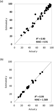

Fig. 6 Comparison of batch and flow syntheses. Plots of actual y vs. estimated y in M1_conv. (a) batch synthesis and (b) flow synthesis.

Examination 1 (search for interpolated regions using double cross validation)

Fig. 7 shows the coefficient of determination (R²) and mean absolute error (MAE) for each objective variable obtained using each regression method. In both models, M1_conv. and M2_conv. had lower R² values and higher MAEs than M1_CR and C_M1_CR when the explanatory variables were process variables (feature set A). Adding one of the feature sets B–D to feature set A improved the prediction accuracy and reduced MAE for all the objective variables. In particular, the prediction accuracy of M1_conv. and M2_conv. improved substantially, with R² values greater than 0.8 irrespective of the regression method. The improvement of the prediction accuracy is attributed to feature set A not containing information that discriminates between monomer types. The radical copolymerization reaction depends on the monomer reactivity ratio for each monomer. Therefore, even if radical polymerization is conducted under similar processing conditions, the rate of the polymerization reaction progress differs depending on the monomer type. The monomer conversion rate is calculated from the monomer concentration remaining in the reaction solution, and is considered to be strongly influenced by the reaction rate. Feature sets B–D differ from each other but all contain information specific to each monomer. The prediction accuracy of monomer conversion in the interpolated region is considered to have been improved as a result. By contrast, the prediction accuracy of M1_CR was relatively high even when only feature set A was used (R² ≈ 0.8). The prediction accuracy of M1_CR was improved when information specific to each monomer (feature sets B–D) was included, and its prediction accuracy was R² > 0.94 for all regression models. The prediction accuracy of M1_CR obtained from the calculation using the monomer conversion rate was high, even though the prediction accuracy of the monomer conversion rate was low when only feature set A was used. Interestingly, C_M1_CR calculated from the predicted monomer conversion showed R² values similar to those of M1_CR calculated from the measured monomer conversion. The reason for the difference in prediction accuracy between monomer conversion and M1_CR is that the monomer composition ratio for a polymer is determined by the ratio between M1_conv. and M2_conv., which suggests that accidental cancellation has occurred (eqn (2)). In addition, the C_M1_CR results indicate that the monomer conversion ratio is not required to be correct to enable the monomer composition ratio for polymers to be predicted. These results suggest that M1_CR is not as dependent on monomer type as monomer conversion but is more dependent on process variables.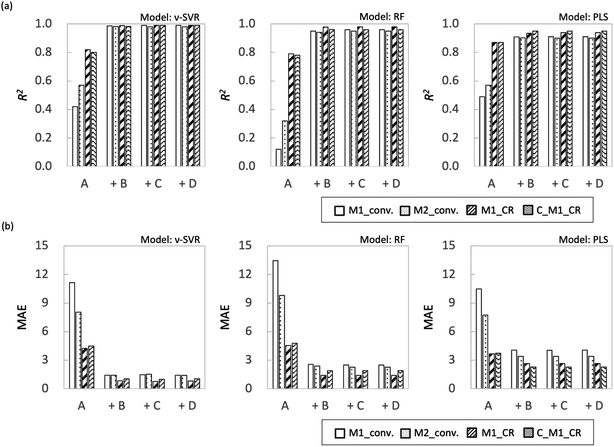

Fig. 7 Plot summarizing prediction results for interpolated regions for each ML algorithm (a) R² and (b) MAE.

With respect to the predictions of monomer conversion in the interpolation region and monomer composition ratio for polymers, we found that creating a learning model using information specific to each monomer (feature sets B–D) improved the prediction accuracy. There were no significant accuracy differences among the predictions of models based on feature sets B–D.

Examination 2 (search for extrapolated regions using molecular extrapolation validation)

Fig. 8 shows R² and MAE for each objective variable obtained using each regression method for extrapolation. As in Examination 1, the R² value for the monomer composition ratio for the polymers was higher than the monomer conversion ratio for all models with the explanatory variable of feature set A; however, the overall accuracy of the prediction was lower. It is not surprising that the training model shows low predictive performance because of the monomer bias. The effect of adding feature sets B–D differed for each model used. The overall trend of the results obtained in this study was that the RF model showed higher prediction accuracy, followed by PLS and ν-SVR, in that order. This result depends on the nonlinearity of the models, with the PLS being a linear model and therefore not fitting the extrapolation region, and the ν-SVR model, which is more nonlinear, showing lower prediction accuracy because regression equation overfitting to the training data is reflected in the extrapolated region.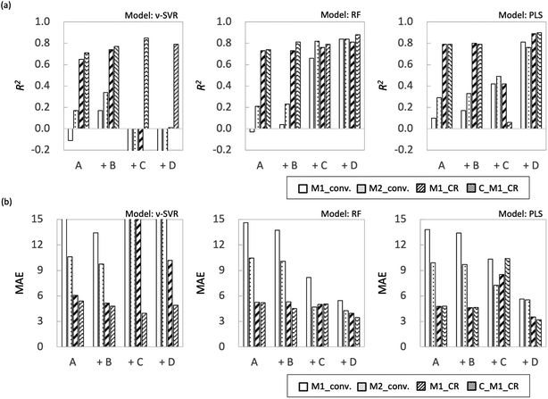

Fig. 8 Plot summarizing prediction results for extrapolation regions for each ML algorithm (a) R² and (b) MAE.

First, in the models with feature set B added to the features, the prediction accuracy of each objective variable increased only for the ν-SVR model; the prediction accuracy of the RF and PLS models showed a decreasing trend. For the ν-SVR model (feature set B), the monomer conversion rate, in particular, was improved; however, its prediction accuracy was insufficient (R² ≈ 0.4). The fact that the predicted values for St and CHMA did not change in any of the models confirms the need to add features other than molecular flags (Fig. S8–S10†). Second, when feature set C was included in the explanatory variable, the prediction accuracy of each objective variable was improved only for the RF model, as in the case of the model with feature set B added. The ν-SVR model reduced the predictions except that for C_M1_CR, whereas the PLS model slightly improved the predictions for the monomer conversion ratio and reduced the predictions for the monomer composition ratio for polymers. The prediction accuracy of monomer conversion was improved compared with that of the RF model (feature set B). Feature set C (RDKit: 208 features) contains more detailed monomer information, including monomer descriptors, monomer molecular weight and the number of rotatable bonds in the monomers. Liu et al. predicted quantum chemical properties using conformers generated from RDKit;³² we therefore expected RDKit to contain information similar to quantum chemical calculations. We assumed that this information would increase the predicted value of the monomer conversion ratio. Because RF is a nonlinear model, its improved accuracy is attributable to the importance of quantum chemical calculations from the fingerprint being implicitly incorporated into the predictive model.

The use of feature set D substantially improved the prediction accuracy of each objective variable in the RF and PLS models. The ν-SVR model showed a trend similar to that observed upon the addition of feature set C. The RF and PLS models showed high prediction accuracy, with R² values of 0.8 or higher for most of the objective variables. For the PLS model, the monomer conversion predictions using feature sets B and C did not change the predicted values of St and CHMA for some of the samples; however, this problem was solved by using feature set D. Feature set B contains only molecular flags and has less information about the characteristics of the monomers. Feature set C details monomer information before the monomer undergoes the radical reaction, such as descriptors and molecular weight, but does not include post-reaction information. However, feature set D mainly describes the electronic energy information when radical reactions occur, along with conformation information about intermediate products (dimers and products of the initiators and monomers) and a large amount of post-reaction information. Radical polymerization is characterized by an increase in the molecular weight of radical molecules as the reaction proceeds; among the feature sets B–D used in the present study, feature set D is considered to best reflect this relationship. Thus, the prediction accuracy of the extrapolation region was substantially improved when feature set D was added. The prediction accuracy of the two models was improved using the energy information in radical reactions calculated via quantum chemical calculations as a feature. These features are expected to be highly versatile and adaptable to various situations. Finally, we calculated important properties to investigate which features contribute to the prediction among feature sets A + D with improved accuracy of the extrapolated regions. This discussion focuses on M1_conv. of the RF model (feature set D), which has superior prediction accuracy for the extrapolated regions. Fig. 9 shows the ten most important features for the M1_conv. prediction in the RF model (feature set D) for various copolymers. In addition, we carried out recursive feature elimination (RFE) using a stepwise method to clearly reveal features with a low learning contribution (Table 1). Herein, the feature number represents the number of features used for training, and the features with the lowest contribution when trained with that number of features are listed. In other words, the smaller the feature number, the higher the contribution of that feature. A total of 41 features are listed in this table: 5 process variables (M1_composition_ratio, initiator_composition_ratio, SM, temperature and flow_rate) and 36 DFT calculated values. M is the M1 monomer, 00 is the M2 monomer, theta (60, 180, 300) is the target value of the dihedral angle created by two C atoms on the radical side and two C atoms on the monomer side, Real_theta is the theta value after TS structural optimization, DE_(00M, M00, MM)_TS_theta (60, 180, 300) is the energy of TS, E_(M, 00)_Rad_(SOMO, LUMO) is the energy of SOMO and LUMO of radicals, E_(M, 00)_Mon_(HOMO, LUMO) is the energy of HOMO and LUMO of monomers, DE_(M, 00)_decomposition_(head, tail) is the energy required to dissociate the initiator from the radical, DE_(00M, M00, MM)_SHgap and DE_(00M, M00, MM)_SLgap are the difference between the two orbital energies. Fig. 9 shows that all of the process variables (feature set A) were included in the top 10 and ranked high irrespective of the monomers used. In particular, flow_velocity showed the highest importance for all the copolymers, followed by temperature, with the combined importance of the two features being greater than 45%. These results indicate that the process variables affect the polymer synthesis. It should also be noted that flow_velocity and temperature, which are of high importance, are set values and do not faithfully represent the inside of the reaction system. Supporting process variables with data on flow velocity and temperature distribution in the design from the fluid simulation is expected to improve the prediction accuracy further. A trend was also observed in feature set D (quantum chemical calculated values) included in the important features. The features included were the HOMO, LUMO and SOMO energies of M1 and M1 radicals, the orbital energy gaps (SOMO–HOMO (SH) gap and SOMO–LOMO (SL) gap) and the energy gaps between the normal state and the transition state. The RFE results indicate that the HOMO, LUMO and SOMO energies of the M2 and M2 radicals, the energy required to dissociate the initiator, and the stereo conformational dihedral angle are less important. Interestingly, the importance of orbital energy with respect to M1 and M2 differed dramatically. Some of the orbital energies related to M1 were definitely included in the ten most important features; however, the four orbital energies related to M2 (variables with the “E_00” suffix) were removed by RFE within six iterations. This result is attributed to MMA being the only monomer that corresponds to M2 and all the copolymers containing MMA. The inclusion of the SH gap and SL gap among the important features indicates that not only the orbital energy of each state but also the difference between them is important. On the basis of these results, the orbital energy related to the monomer in the extrapolation region and the orbital energy gap between the monomer and the radical were concluded to be important features for predicting polymerization using monomers not included in the learning.

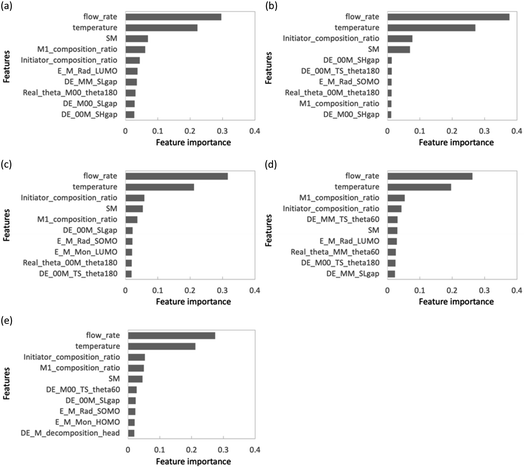Fig. 9 Feature importance chart for each copolymer in feature sets A + D: (a) GMA, (b) St, (c) PACS, (d)THFMA and (e) CHMA.

Table 1 List of deleted features using RFE

Feature number	GMA	St	PACS	THFMA	CHMA
41	E_00_Rad_LUMO	E_00_Mon_HOMO	DE_00_decomposition_tail	DE_00_decomposition_head	E_00_Rad_SOMO
40	E_00_Mon_LUMO	E_00_Rad_LUMO	DE_00_decomposition_head	E_00_Rad_SOMO	E_00_Rad_LUMO
39	E_00_Mon_HOMO	E_00_Rad_SOMO	E_00_Mon_LUMO	E_00_Rad_LUMO	DE_00_decomposition_tail
38	DE_00_decomposition_tail	DE_00_decomposition_tail	E_00_Mon_HOMO	E_00_Mon_LUMO	DE_00_decomposition_head
37	DE_00_decomposition_head	DE_00_decomposition_head	E_00_Rad_LUMO	E_00_Mon_HOMO	E_00_Mon_LUMO
36	E_00_Rad_SOMO	E_00_Mon_LUMO	E_00_Rad_SOMO	DE_00_decomposition_tail	E_00_Mon_HOMO
35	DE_M_decomposition_tail	Real_theta_00M_theta300	DE_MM_SHgap	DE_00M_SLgap	Real_theta_M00_theta300
34	DE_MM_SHgap	Real_theta_M00_theta60	DE_M_decomposition_tail	Real_theta_M00_theta300	Real_theta_M00_theta60
33	Real_theta_MM_theta180	DE_MM_TS_theta180	Real_theta_MM_theta60	Real_theta_M00_theta180	Real_theta_MM_theta180
32	Real_theta_MM_theta60	DE_M_decomposition_tail	Real_theta_00M_theta300	E_M_Mon_LUMO	DE_MM_SHgap
31	Real_theta_M00_theta60	Real_theta_MM_theta60	Real_theta_M00_theta300	Real_theta_00M_theta60	Real_theta_MM_theta60
30	Real_theta_00M_theta300	Real_theta_M00_theta300	Real_theta_MM_theta180	Real_theta_MM_theta180	DE_MM_TS_theta180
29	Real_theta_M00_theta300	E_M_Mon_LUMO	Real_theta_M00_theta180	DE_M_decomposition_tail	Real_theta_M00_theta180
28	E_M_Mon_LUMO	DE_00M_SLgap	Real_theta_M00_theta60	Real_theta_00M_theta300	DE_M_decomposition_tail
27	DE_MM_TS_theta180	DE_MM_SHgap	Real_theta_00M_theta60	Real_theta_MM_theta300	Real_theta_00M_theta60
26	DE_00M_SLgap	Real_theta_M00_theta180	DE_MM_SLgap	DE_M00_SHgap	DE_00M_TS_theta300
25	DE_M00_TS_theta60	Real_theta_MM_theta180	E_M_Mon_HOMO	Real_theta_00M_theta180	E_M_Rad_LUMO
24	DE_MM_TS_theta60	Real_theta_00M_theta60	DE_00M_TS_theta60	E_M_Rad_SOMO	DE_00M_SHgap
23	DE_00M_TS_theta60	DE_M00_TS_theta180	DE_MM_TS_theta300	E_M_Mon_HOMO	DE_M00_TS_theta180
22	E_M_Rad_SOMO	Real_theta_MM_theta300	Real_theta_MM_theta300	DE_00M_TS_theta300	DE_00M_SLgap
21	DE_M00_TS_theta180	DE_00M_TS_theta300	DE_00M_TS_theta300	DE_MM_TS_theta300	E_M_Mon_LUMO
20	DE_M00_TS_theta300	DE_M00_TS_theta300	DE_M00_SLgap	DE_00M_SHgap	DE_M00_SLgap
19	E_M_Mon_HOMO	DE_MM_TS_theta60	E_M_Rad_LUMO	DE_MM_TS_theta180	DE_M00_SHgap
18	Real_theta_MM_theta300	E_M_Rad_LUMO	Real_theta_00M_theta180	DE_M_decomposition_head	Real_theta_MM_theta300
17	DE_M_decomposition_head	M1_composition_ratio	DE_MM_TS_theta60	DE_MM_TS_theta60	DE_MM_SLgap
16	DE_00M_TS_theta180	DE_M00_TS_theta60	DE_M00_TS_theta180	SM	DE_M_decomposition_head
15	DE_00M_TS_theta300	DE_00M_TS_theta60	E_M_Mon_LUMO	DE_00M_TS_theta180	E_M_Rad_SOMO
14	DE_MM_TS_theta300	DE_MM_SLgap	E_M_Rad_SOMO	E_M_Rad_LUMO	Real_theta_00M_theta180
13	Real_theta_00M_theta180	E_M_Mon_HOMO	DE_M_decomposition_head	DE_MM_SHgap	Real_theta_00M_theta300
12	E_M_Rad_LUMO	DE_00M_TS_theta180	M1_composition_ratio	DE_00M_TS_theta60	DE_MM_TS_theta300
11	Initiator_composition_ratio	DE_M_decomposition_head	DE_M00_SHgap	Initiator_composition_ratio	SM
10	DE_MM_SLgap	DE_M00_SLgap	DE_M00_TS_theta300	DE_M00_TS_theta180	E_M_Mon_HOMO
9	DE_M00_SHgap	DE_M00_SHgap	SM	DE_M00_SLgap	Initiator_composition_ratio
8	SM	Real_theta_00M_theta180	DE_MM_TS_theta180	M1_composition_ratio	DE_MM_TS_theta60
7	M1_composition_ratio	E_M_Rad_SOMO	Initiator_composition_ratio	DE_MM_SLgap	M1_composition_ratio
6	DE_M00_SLgap	SM	DE_M00_TS_theta60	Real_theta_MM_theta60	DE_00M_TS_theta180
5	Real_theta_00M_theta60	Initiator_composition_ratio	DE_00M_SLgap	DE_M00_TS_theta300	DE_00M_TS_theta60
4	DE_00M_SHgap	DE_MM_TS_theta300	DE_00M_TS_theta180	DE_M00_TS_theta60	DE_M00_TS_theta60
3	Temperature	DE_00M_SHgap	Temperature	Temperature	Temperature
2	Flow_rate	Temperature	Flow_rate	Flow_rate	Flow_rate
1	Real_theta_M00_theta180	Flow_rate	DE_00M_SHgap	Real_theta_M00_theta60	DE_M00_TS_theta300

---

Conclusions

Five binary copolymers were radically polymerized under various process conditions using a flow reactor, and the obtained experimental results were analysed by ML. Two training–test splits were performed to represent either the interpolated or extrapolated region predictions for monomers, and three regression methods (ν-SVR, RF and PLS) were used for each dataset to make predictive models for the monomer conversion and the monomer composition ratio for polymers. When interpolated regions were represented by double cross validation, the process variables during copolymer synthesis (feature set A) and any of the features characterizing the monomer (feature sets B–D) were used as explanatory variables, and all the regression methods showed high prediction accuracy. Extrapolation regions were expressed by molecular extrapolation validation, and the prediction accuracy was improved only under the condition where theoretically calculated values (feature set D) were added to the process variables as explanatory variables. Most of the monomer composition ratios for the polymers calculated using the predicted values for monomer conversion were as accurate or more accurate than those predicted using the measured values for monomer conversion. As described, the monomer conversion ratio and the monomer composition ratio for polymers, including the extrapolated region, can be predicted by combining experimental conditions and quantum chemical calculation values.

We found that the molecular orbital energy information for the monomer (extrapolated region) and the orbital energy gap with radicals are necessary for highly accurate prediction of the extrapolated region. It is thought that the inclusion of features using quantum chemical calculations in anionic polymerization, cationic polymerization, polycondensation, and radical polymerization will enable the prediction of extrapolation regions. In such cases, it is necessary to conduct highly reproducible experiments, such as those involving the flow reactor used in this study. However, polymerization using flow reactors is difficult for reactions such as polycondensation, in which the viscosity increases rapidly. Hence, it is necessary to find a reactor that can obtain highly reproducible results for each synthesis method. The proposed model is expected to accelerate the development of polymers using new monomers.

Data availability

The participants of this study did not give written consent for their data to be shared publicly, so due to the sensitive nature of the research supporting data is not available.

Author contributions

S. Takasuka: investigation (ML, EXP), writing – original draft. S. Oikawa: investigation (ML). T. Yoshimura: investigation (QC). S. Ito: investigation (ML, EXP). Y. Harashima: resources. T. Takayama: formal analysis (EXP). S. Asano: investigation (EXP). A. Kurosawa: investigation (EXP). T. Sugawara: conceptualization (EXP), formal analysis (EXP). M. Hatanaka: formal analysis (QC). T. Miyao: formal analysis (ML). T. Matsubara: supervision (ML). Y. Ohnishi: formal analysis (QC). H. Ajiro: investigation (EXP). M. Fujii: project administration, where ML, QC, and EXP represent the machine learning, quantum chemistry calculations, and experiments.

Conflicts of interest

The authors declare no competing financial interest.

Acknowledgements

This paper is based on results obtained from a project, JPNP14004, subsidized by the New Energy and Industrial Technology Development Organization (NEDO) and JSPS KAKENHI Grant Number JP21K20537.

References

1. E. A. Eastwood and M. D. Dadmun, Macromolecules, 2001, 34, 740.
2. I. Piirma and L. P. H. Chou, J. Appl. Polym. Sci., 1979, 24, 2051.
3. Y. Kotani, M. Kamigaito and M. Sawamoto, Macromolecules, 1998, 31, 5582.
4. J. Schweer, Macromol. Theory Simul., 1993, 2, 485.
5. D. Neugebauer, K. Bury and M. Wlazło, J. Appl. Polym. Sci., 2012, 124, 2209.
6. J. Handique, B. Jyoti Saikia and S. Kumar Dolui, Polym. Sci., Ser. A, 2019, 61, 577.
7. X. Fei, Y. Shi and Y. Cao, Appl. Phys. A, 2010, 100, 409.
8. W. Trehern, R. Ortiz-Ayala, K. C. Atli, R. Arroyave and I. Karaman, Acta Mater., 2022, 228, 117751.
9. A. Shafe, C. D. Wick, A. J. Peters, X. Liu and G. Li, Polymer, 2022, 242, 124577.
10. A. Ihalage and Y. Hao, Adv. Sci., 2022, 9, 2200164.
11. S. P. Mishra and M. R. Rahul, Comput. Mater. Sci., 2021, 200, 110815.
12. R. Machaka, Comput. Mater. Sci., 2021, 188, 110244.
13. J. A. Pugar, C. Gang, C. Huang, K. W. Haider and N. R. Washburn, ACS Appl. Mater. Interfaces, 2022, 14, 16568.
14. J. Hu, S. Stefanov, Y. Song, S. Sadeed Omee, S. Y. Louis, E. M. D. Siriwardane, Y. Zhao and L Wei, npj Comput. Mater., 2022, 8, 65.
15. D. Santacruz, F. O. Enane, K. Fundel-Clemens, M. Giner, G. Wolf, S. Onstein, C. Klimek, Z. Smith, B. Wijayawardena and C. Viollet, SLAS Discovery, 2022, 27, 140.
16. K. Y. Nandiwale, T. Hart, A. F. Zahrt, A. M. K. Nambiar, P. T. Mahesh, Y. Mo, M. José Nieves-Remacha, M. D. Johnson, P. García-Losada, C. Mateos, J. A. Rincónb and K. F. Jensen, React. Chem. Eng., 2022, 7, 1315–1327.
17. L. Brocken, P. D. Price, J. Whittaker and I. R. Baxendale, React. Chem. Eng., 2017, 2, 662.
18. L. Yang, J. A. Haber, Z. Armstrong, S. J. Yang, K. Kan, L. Zhou, M. H. Richter, C. Roata, N. Wagnera, M. Corama, M. Berndla, P. Rileya and J. M. Gregoire, Proc. Natl. Acad. Sci. U. S. A., 2021, 118, e2106042118.
19. G. Luca Losacco, H. Wang, I. A. H. Ahmad, J. Dasilva, A. A. Makarov, I. Mangion, F. Gasparrini, M. Lämmerhofer, D. W. Armstrong and E. L. Regalado, Anal. Chem., 2022, 94, 1804.
20. R. Bennett, R. D. Cohen, H. Wang, T. Pereira, M. A. Haverick, J. W. Loughney, D. C. Barbacci, P. Pristatsky, A. M. Bowman, G. Luca Losacco, D. D. Richardson, I. Mangion and E. L. Regalado, Anal. Chem., 2022, 94, 1678.
21. C. W. Coley, D. A. Thomas, J. A. M. Lummiss, J. N. Jaworski, C. P. Breen, V. Schultz, T. Hart, J. S. Fishman, L. Rogers, H. Gao, R. W. Hicklin, P. P. Plehiers, J. Byington, J. S. Piotti, W. H. Green, A. John Hart, T. F. Jamison and K. F. Jensen, Science, 2019, 365, eaax1566.
22. Y. Zhou, Y. Gu, K. Jiang and M. Chen, Macromolecules, 2019, 52, 5611.
23. M. H. Reis, F. A. Leibfarth and L. M. Pitet, ACS Macro Lett., 2020, 9, 123.
24. B. A. Rizkin, A. S. Shkolnik, N. J. Ferraro and R. L. Hartman, Nat. Mach. Intell., 2020, 2, 200.
25. M. Rubens, J. H. Vrijsen, J. Laun and T. Junkers, Angew. Chem., Int. Ed., 2019, 58, 3183.
26. M. Reis, F. Gusev, N. G. Taylor, S. Hun Chung, M. D. Verber, Y. Z. Lee, O. Isayev and F. A. Leibfarth, J. Am. Chem. Soc., 2021, 143, 17677.
27. J. da Tan, B. Ramalingam, S. Liang Wong, J. Cheng, Y. F. Lim, V. Chellappan, S. A. Khan, J. Kumar and K. Hippalgaonkar, ChemRxiv, 2022, preprint,  DOI:10.26434/chemrxiv-2022-tlz53.
28. A. Wakiuchi, S. Takasuka, S. Asano, R. Hashizume, A. Nag, M. Hatanaka, T. Miyao, Y. Ohnishi, T. Matsubara, T. Ando, T. Sugawara, M. Fujii and H. Ajiro, Macromol. Mater. Eng., 2022, 2200626.
29. B. Gu, V. S. Sheng, Z. Wang, D. Ho, S. Osmanh and S. Li, Neural Network., 2015, 67, 140.
30. T. Akiba, S. Sano, T. Yanase, T. Ohta and M. Koyama, Proc. KDD'19, 2019,  DOI:10.1145/3292500.3330701.
31. RDKit. Open-source cheminformatics, https://www.rdkit.org, accessed October 2021.
32. M. Liu, C. Fu, X. Zhang, L. Wang, Y. Xie, H. Yuan, Y. Luo, Z. Xu, S. Xu and S. Ji, arXiv, 2021, preprint, arXiv:2106.08551,  DOI:10.48550/arXiv.2106.08551.

---

Footnote

† Electronic supplementary information (ESI) available. See DOI: https://doi.org/10.1039/d2dd00144f

---