 Open Access Article
Creative Commons Attribution 3.0 Unported Licence
Predicting ruthenium catalysed hydrogenation of esters using machine learning†
Challenger
Mishra
*a,
Niklas
von Wolff
 *b,
Abhinav
Tripathi
c,
Claire N.
Brodie
 c,
Neil D.
Lawrence
a,
Aditya
Ravuri
a,
Éric
Brémond
 d,
Annika
Preiss
c and
Amit
Kumar
 *c
*c
aDepartment of Computer Science and Technology, University of Cambridge, Cambridge, CB30FD, UK. E-mail: cm2099@cam.ac.uk
bLaboratoire d'Electrochimie Moléculaire, Université Paris Cité, CNRS, F-75006 Paris, France. E-mail: niklas.von-wolff@u-paris.fr
cSchool of Chemistry, University of St. Andrews, St. Andrews, KY169ST, UK. E-mail: ak336@st-andrews.ac.uk
dITODYS, Université Paris Cité, CNRS, F-75006 Paris, France
First published on 1st May 2023
Abstract
Catalytic hydrogenation of esters is a sustainable approach for the production of fine chemicals, and pharmaceutical drugs. However, the efficiency and cost of catalysts are often bottlenecks in the commercialization of such technologies. The conventional approach to catalyst discovery is based on empiricism, which makes the discovery process time-consuming and expensive. There is an urgent need to develop effective approaches to discover efficient catalysts for hydrogenation reactions. In this work, we explore the approach of machine learning to predict outcomes of catalytic hydrogenation of esters using various ML architectures – NN, GP, decision tree, random forest, KNN, and linear regression. Our optimized models can predict the reaction yields with reasonable error for example, a root mean square error (RMSE) of 11.76% using GP on unseen data and suggest that the use of certain chemical descriptors (e.g. electronic parameters) selectively can result in a more accurate model. Furthermore, studies have also been carried out for the prediction of catalysts and reaction conditions such as temperature and pressure as well as their validation by performing hydrogenation reactions to improve the poor yields described in the dataset.
1 Introduction
The catalytic hydrogenation of esters to alcohols is an atom-economic and sustainable approach in organic synthesis with significant applications in the production of various fine chemicals such as detergents, cosmetics, flavors, fragrances, and pharmaceutical drugs.1 The concept has also been expanded to the hydrogenation of polyesters to enable a circular economy.2 In the past, several homogeneous and heterogeneous catalysts have been developed, among which well-defined ruthenium complexes represent the state-of-the-art catalysts for the hydrogenation of esters to alcohols.1,3 However, most of such catalysts exhibit low TONs (e.g. <200), and operate under harsh conditions (e.g. temperature > 100 °C, and pressure > 20 bars) making this approach expensive and incompatible for molecules containing other sensitive or reducible functional groups. Thus, the true utilization of hydrogenation methodology relies on finding an optimum catalyst that can hydrogenate an ester with high activity and selectivity under mild conditions (e.g., room temperature, and ambient pressure). Our current conventional approach to catalysis development fails to achieve this due to a number of limitations such as (a) empirical screening of several parameters such as solvent, temperature, pressure, time, additive, etc. can only be limited to a certain extent, (b) syntheses of well-defined ruthenium catalysts often involve complex multi-step processes limiting the scope of complexes that can be studied, (c) lack of mechanistic understanding of new complexes limits its application in catalysis, and (d) intrinsic limitation of the human brain to find a pattern in large data collections restricts us to a smaller dataset. Chemoinformatics provides an attractive alternative to the conventional empirical approach. Although a mechanistic understanding of the underlying class of reactions can be highly beneficial in such a venture, it is possible to find patterns in large datasets of chemical reactions even without mechanistic knowledge. This can be accomplished by deploying novel machine-learning methodologies and architectures tailored to such applications.4 This can facilitate the discovery of desirable catalyst designs and catalytic conditions, bypassing the complexity of empirical synthesis and screening.5–7Although powerful, the application of the tool of machine learning (ML) in the discovery of molecular catalysts is in its nascent phase and growing.7–11 A few reports have been published on the development of predictive models for catalytic reactions using various machine learning architectures dictated by the nature of the reaction, molecular catalyst, and available dataset. For example, Kozlowski utilized Quantitative Structure Selectivity Relationship (QSSR) models for the prediction of the catalytic alkylation of aldehydes using beta-amino alcohol catalysts.12 Sigman and co-workers have developed predictive models for several asymmetric catalytic reactions using multivariate regression models.13–21 Along this direction, Doyle, and co-workers have used a random forest model to predict the yield of catalytic C–N cross-coupling reactions.22 Denmark has recently reported a computationally guided workflow and a highly accurate predictive model for the chiral phosphoric-acid catalysed thiol addition to N-acylimines using deep feed-forward neural networks.23 A predictive model for the asymmetric hydrogenation of alkenes and imines catalysed by chiral binapthyl catalysts has been recently reported by Sunoj where a root-mean-square error (RMSE) of about 8.4 ± 1.8% was obtained using a random forest model.24
Most of the studies on the prediction of catalytic reactions in the literature involve linear regression, decision tree, artificial neural networks, K-nearest neighbors, and random forest. Another model called the Gaussian process, noteworthily, has not been utilized to model a homogeneous catalytic reaction. Gaussian processes are non-parametric machine learning models where the functions are fitted to the data in a Bayesian framework.25 The main advantage of using a Gaussian process over other machine learning models is that it can automatically provide uncertainty information since its predictions are distributions. Uncertainty information can be particularly useful in case of a small and skewed dataset. The main computational bottleneck in making inferences using GPs (Gaussian Processes) is inverting matrices which are the size of the dataset. The relatively small size of a dataset can be thus particularly suited for an approach using Gaussian processes. Furthermore, GP provides the information of length scales and Gaussian noise which tells us if the model is learning or treating the data as noise. It also tells us the importance of various features. This information can be useful if the dataset is small and not very systematic.26
Considering the contemporary interests in developing sustainable catalysts for the hydrogenation of esters, we report here the application of ML (Machine Learning) tools, specifically Gaussian processes, to predict the outcome of ester hydrogenation using well-defined ruthenium catalysts. Our approach involves the following three steps: (1) dataset construction, and exploratory data analysis, (2) creation of chemical descriptors for catalysts, and esters, and (3) development of predictive models using ML frameworks such as neural networks (NNs), and Gaussian processes (GPs). We also compare machine learning models with a baseline linear model. The linear model is also trained in a Bayesian framework by using a Gaussian process model with a linear kernel.
2 Results and discussion
2.1 Dataset construction
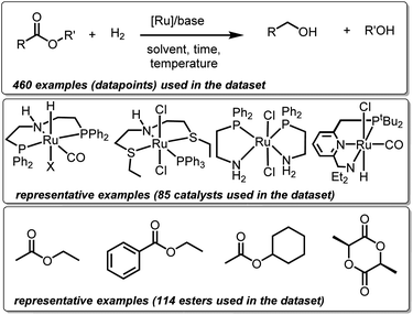
We created a dataset of reactions involving hydrogenation of esters by well-defined ruthenium complexes from existing (peer-reviewed) literature. This choice is guided by two factors. Firstly, homogeneous ruthenium catalysts are known for their high activity towards hydrogenation of esters making this family a suitable choice for potential superior future catalysts. Secondly, substantial research outputs in the past on several types of ruthenium catalysts present sufficient data needed for ML studies.27 Only those examples have been included in the dataset where the structures of ruthenium catalysts are well-defined, and where the reaction medium is either neutral or basic. Mechanistically, all the catalysts (with a few exceptions) have been proposed to operate via non-redox metal–ligand cooperation. Thus, our dataset consists of 460 hydrogenation reactions involving 85 ruthenium catalysts and 114 esters and lactones (Fig. 1). Each reaction or datapoint is characterized by 12 broad sets of parameters – catalyst structure, ester structure, amount of ester (mmol), catalyst loading (mol%), base structure, base loading (mol%), temperature (°C), pressure of H2 (bar), reaction time (h), solvent structure, solvent amount (mL), and yield (%).2.2 Creation of chemical descriptors
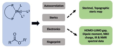
In order to successfully use the dataset to develop a generalizable ML model, it is important to transform the structures and properties of catalysts, esters, bases, and solvents into informative numbers called chemical descriptors as also recently highlighted by Grzybowski and co-authors.28 Significant work has been done in the past on the development of various types of chemical descriptors and their importance for the development of ML models for catalytic reactions as reviewed by Fey and co-workers.29–32 Lapkin and co-workers have recently reported an interesting study on the effect of chemical representation on machine learning models for the reaction optimisation and suggest that the success of various chemical descriptors depend on various factors such as the complexity of chemistry, the dimensionality of the design space and the number of variables.33 Aspuru-Guzik and Balcells have used graph or connectivity-based chemical descriptor computed using autocorrelation function and DFT optimized structures for Vaska-type H2-activation.34 The choice of descriptors and whether they are derived from DFT calculations, experiments, or even other ML models, often depends on the size of the available dataset. In general, there is a trade-off between descriptor accuracy and computational cost. In the case of large datasets, graph or connectivity-based descriptors can be used successfully in ML approaches with minimum computational cost.34 In the present work, however, the design of suitable descriptors is challenging due to the small size of the dataset, the variety of ligand architectures and their complex geometries, the known importance of solvent interactions in the studied catalysts operating through metal–ligand cooperation,35–38 as well as unknown mechanisms and involvement of several rate-limiting states.39–41 We, therefore, used a combination of DFT-based as well as experimentally estimated descriptors (spectral data) in addition to readily accessible graph-based descriptors (Fig. 2). Catalysts have been represented by three types of chemical descriptors. The first type is the graph-based descriptor calculated using an autocorrelation function of depth 4.34 The second type is sterics-based descriptors calculated using (a) topographic steric maps (% Vfree, % Vquadr.free) through DFT-optimized structures and the Morfeus software (buried volumes and solvent accessible surface area and volumes). The third one is electronics-based descriptors calculated using DFT (HOMO–LUMO gap, dipole moment, as well as the NBO charge on the central Ru-atom). Similarly, the ester substrates have also been represented by three types of chemical descriptors: (a) graph-based descriptors using an autocorrelation function of depth 4,34 (b) sterics-based descriptors (sterimol parameters and solvent accessible area and volume), and (c) electronics-based descriptors (HOMO–LUMO gap, dipole moment, C![[double bond, length as m-dash]](https://www.rsc.org/images/entities/char_e001.gif) O-stretching frequency and intensity, and NMR chemical shifts). Solvents and the nature of bases have also been found to play important roles in the catalytic output for this type of reaction, and we, therefore, included relevant descriptors: dielectric constants and Gutmann donor numbers for the solvents, whereas bases were represented by their pK-values (see ESI† for more details). Additionally, solvents and base were also represented by one-hot-encoding. We also used RD-Kit, Morgan, and MACCS-based fingerprints for esters, solvents and bases.
O-stretching frequency and intensity, and NMR chemical shifts). Solvents and the nature of bases have also been found to play important roles in the catalytic output for this type of reaction, and we, therefore, included relevant descriptors: dielectric constants and Gutmann donor numbers for the solvents, whereas bases were represented by their pK-values (see ESI† for more details). Additionally, solvents and base were also represented by one-hot-encoding. We also used RD-Kit, Morgan, and MACCS-based fingerprints for esters, solvents and bases.
2.3 Development of predictive models for the catalytic hydrogenation of esters
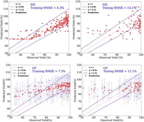 | ||
| Fig. 3 Prediction of yields for the catalytic hydrogenation of esters using NN (top row) and GP (bottom row) for the dataset containing yield > 50%. | ||
| Model | Train RMSE (%) | Test RMSE (%) | Train R2 | Test R2 |
|---|---|---|---|---|
| Gaussian processes | 8.55 ± 1.05 | 11.76 ± 0.84 | 0.57 ± 0.08 | 0.09 ± 0.09 |
| Decision trees | 11.55 ± 0.31 | 12.02 ± 0.81 | −8.55 ± 2.24 | −9.75 ± 4.45 |
| Random forest | 4.18 ± 0.01 | 13.60 ± 0.01 | 0.75 ± 0.02 | −2.26 ± 0.80 |
| K nearest neighbours | 11.50 ± 0.39 | 12.04 ± 0.95 | −10.47 ± 2.26 | −12.34 ± 3.78 |
| Mean model | 12.11 ± 0.35 | 12.38 ± 0.79 | 0.00 ± 0.00 | −0.02 ± 0.022 |
Furthermore, using linear regression (LR), a similar RMSE of 12.7% was obtained for the test set (yields > 50%). Although the result metrics of the linear model and Gaussian process model are very similar, the hyperparameter – Gaussian noise variance-is 9 times the order of linear kernel variance, indicating that the linear model is learning the data as noise. In the case of the Matern52 kernel model, the Gaussian noise variance is of the same order as the Matern52 kernel variance (Table S6; the GP Section 3.2.1 in the ESI discusses the hyperparameters, Fig. S3† shows length-scales of Matern52 kernel). Evaluating the metrics of performance on the test set should be done in conjunction with the resulting optimal hyperparameter values. Gaussian process models provide a natural interpretation of the model's hyperparameters, as length-scales in the input domain over which the model's outputs vary. In this sense, a GP is much more interpretable in comparison to our neural network model. To make the dataset contain both good and bad points, we used the dataset in the yield range of 30–70% and 40–65%, however, the results were not any better than that of yield > 50% (see below and ESI, Table S13†). Furthermore, we found that the prediction of our ML models is not significantly better than a benchmark model (called as mean model, Table 1) that gives a constant prediction which is the mean of the output of the training dataset. A similar observation has also been made recently by Burke and Grzybowski where they advocated that the results from ML models are not significantly better than such simple models for cases where the dataset is created from the literature reports.42 This is mainly due to the biased nature of the dataset likely because of the preference of chemists to use specific protocols, availability/cost of certain reagents, and the practice of not reporting failed experiments as also pointed out in recent reports by Vuilleumier,43 and Glorius.44 Regardless, the approach of ML can provide several information useful to chemists which cannot be done using a simple mean model, such as the relative importance of descriptors and prediction of catalysts using a classification setting as described in the following sections.
We studied the importance of chemical descriptors using our ML modes. In total, 64 datasets were created using various combinations of descriptors (Fig. 2, and see ESI, Table S3†) as well as including cases where no chemical descriptor is used. Our experiments showed that the lowest RMSE is obtained by using autocorrelation and steric parameters of esters and autocorrelation parameters of catalysts (Fig. 4). The autocorrelation parameter is a relatively complex descriptor that involves structural features calculated by taking into account atomic properties such as electronegativity and the size of individual atoms.34 These fundamental properties can be considered as molecular fingerprints and therefore they are likely to have a substantial effect on the model's performance. Additionally, the length scales of a trained Gaussian process model were used to determine the relative importance of individual features. The ARD (Automatic Relative Determination) feature of the GPy library allows assigning different length-scales to different features during the optimisation step. This also shows that the autocorrelation parameters are the most important features (see ESI, Table S10†). We also carried out leave-one-out studies, where one feature (out of total 84 features) was left out individually while optimising the model to understand its impact on the prediction error. Our studies showed only a slight change in error when removing a specific feature (1–2%, Table S11, ESI†).
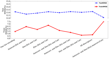 | ||
| Fig. 4 Plot of test/train RMSE with different descriptors using Matern52 kernel. (Autocorr.: autocorrelation, Ster.: sterics, Elec: electronics, Est.: esters, Cat.: catalyst). | ||
Interestingly, just using one-hot encoding to represent catalysts and esters (without using any chemical descriptors) also resulted in an RMSE of 13.2% (on the test set), only marginally higher than our best result of 11.76% using selected descriptors (Fig. 4). Additionally, when bases, solvents, and esters were represented only by molecular fingerprints such as RD-Kit, Morgan, and MACCS-based descriptors, keeping catalysts descriptors the same as previously described (autocorrelation, sterics, and electronics parameters), results were not much different than the best results obtained using selected descriptor (11.76%, RMSE on the test set, see ESI, Table S9†). We acknowledge that our dataset has a large number of data points in the high-yield region compared to low the yield region. We, therefore, hypothesized that using a more balanced dataset containing data points from both high and low-yield regions (e.g. 30–70% or 40–80%) could lead to higher accuracy. In the case of using a dataset of the yield region 40–80%, the results (testing RMSE: 12.31 ± 1.06%) were similar to our optimised result (testing RMSE: 11.76%, yield > 0.5). In other cases, the accuracy was worse than this as mentioned in Table S13.† We also created a more balanced dataset where 50% of the data was randomly picked from the yield ≤ 60% and 50% from the yield ≥ 50%. However, this led to poorer accuracy in the prediction of yield (31.16 ± 3.11 (test)).
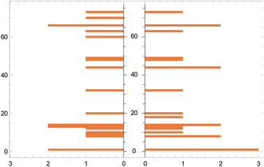 | ||
| Fig. 5 Histogram of actual (left) vs. predicted (right) catalysts. The vertical axis represents the catalyst 1–85 (Section 1.1, ESI†) and the horizontal axis represents their frequency. The gaps on the vertical axis arise when a catalyst is present in either the training set or a test set. | ||
We employed a simple MLP (multilayer perceptron) architecture and linear regression to predict various catalyst descriptors. In total, we have 8 steric descriptors and three electronic descriptors. Since neural networks are good at making end-to-end predictions, we attempted to predict all these features simultaneously. We conducted two different sets of experiments. In the first set of experiments [Expt. A], we divided our dataset into a train-test split of 80–20 and built an MLP model that aims to predict all such catalyst descriptors simultaneously (Section 3.5 of ESI†). We compared our outcomes against linear models (realized through linear regression) for each of these features. In the second set of experiments [Expt. B], we divided the dataset into two disjoint parts such that each catalyst features in exactly one of the sets. This is in line with our goal of predicting new catalysts or their properties. We discovered that our models are good at predicting certain steric and electronic properties of catalysts. These are buried volume, solvent-accessible surface area, and volume (SASA). Similarly, both the linear and the MLP models do quite well in predicting the HOMO–LUMO gap of the catalysts (>90% test accuracy, see Table S14 in the ESI†). In Fig. S10 and S11 in the ESI† we present a plot of true vs. predicted HOMO–LUMO gaps and buried volumes of catalysts from our models, showing a strong agreement. We state at the outset that our efforts in this direction have not yielded in predictions of high accuracy for a majority of descriptors. This is largely in part due to the limited nature of the data available, for example, the heterogeneous distribution of yields (Fig. S1†), and the manifestation of human errors in the dataset curated from the literature.
To probe further, we studied a part of the dataset containing 30 experiments that correspond to a homogeneous yield distribution. Interestingly, a Gaussian process with a Weisfeiler–Lehman graph kernel (Fig. S5†) using SMILES-based descriptors for catalysts and esters was able to significantly outperform Gaussian processes with linear kernels (RMSE: training 4.7%, test 6.1%) that used chemical descriptors as inputs (e.g., autocorrelation, sterics, and electronics) with a limited variation between validation splits (RMSE: training 2–5%, testing: 6–15%). We believe our efforts in this direction would likely benefit from incorporating domain expertise as priors to our GP models, which we have thus far not fully exploited.
In addition to the prediction of yields and catalysts, we were also interested to find if our model can predict the reaction conditions such as – temperature and pressure, which could be of significant benefit to a synthetic chemist while designing catalytic reactions. Remarkably, we found that our model was able to predict pressure with high accuracy (RMSE testing: 3.3% using GP) however a relatively low prediction accuracy was obtained for temperature (RMSE testing: 17.6.% using GP). Fig. 6 and 7 show the prediction of pressure and temperature respectively using linear models and GP. As shown in these figures, the GP model outperforms the linear model and can capture the non-linearity in the dataset.
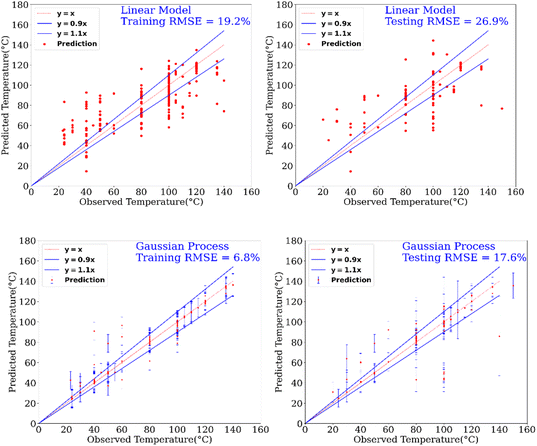 | ||
| Fig. 6 Prediction of temperature of reactions using a linear model and a GP model. This experimental setup corresponds to Expt. B, detailed in Section 3.2.2 (ESI†) for cut-off yield γ = 0.5. | ||
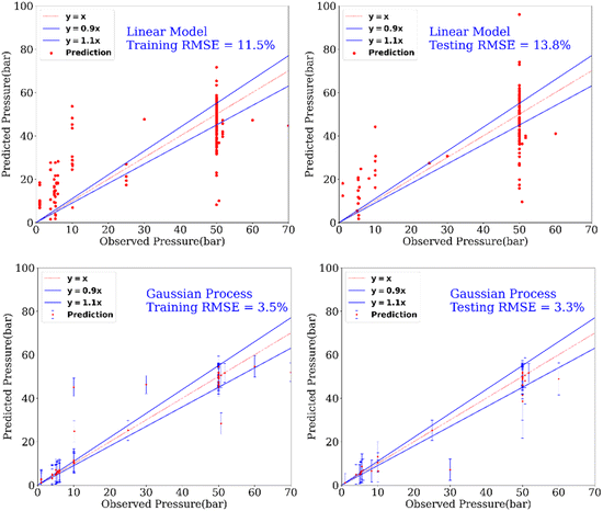 | ||
| Fig. 7 Prediction of the pressure of reactions using a linear model and a GP model. This experimental setup corresponds to Expt. A, detailed in Section 3.2.2 (ESI†) for cut-off yield γ = 0.5. | ||
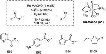
Finally, we carried out some studies on the partial validation of our model. We do not report here the ultimate validation that will be to predict a new catalyst and catalytic conditions to obtain quantitative yields for the hydrogenation of challenging esters under mild conditions due to the complexity of problem and acknowledging the limitations of our dataset curated from literature. However, as a preliminary proof of concept, we aim to use the features (e.g. catalysts, esters, and catalytic conditions) within the dataset to explore if our model can assist in improving the yields of the hydrogenation of esters from the dataset. We picked those esters (E59, E82, E84, E105) that were commercially available and where reported yields in literature were less than 30%. We predicted the yields for the hydrogenation of these esters under the conditions: Ru-MACHO catalyst (C1, 1 mol%), KOtBu (2 mol%), H2 (40 bar), 100 °C, 24 h, and THF (2 mL). We chose some of these conditions as our model predicted them to be a more suitable condition for obtaining higher yield for the hydrogenation reaction (Fig. 5–7). Delightfully, when we performed experiments under the catalytic conditions used for prediction, three out of four esters resulted in higher yields of alcohols in comparison to the literature yields and closer to the predicted yields (Table 2, see ESI Section 4.2† for more details).
| Ester | Conversiona/% | Yieldb/% | Literature yield/% | Predicted yield/% |
|---|---|---|---|---|
| a Determined by GC-MS. b 1H NMR yield using internal standard [1,1′-diphenylethylene]. c Determined by 1H NMR spectroscopy due to poor peak shapes in the GC-MS obtained. | ||||
| E59 | >99 | 96 | 3 (ref. 14) | 95.4 |
| E82 | 63c | 63 | 0 (ref. 15) | 86 |
| E84 | <1 | <1 | 0 (ref. 15) | 84 |
| E105 | >99 | 99 | 32 (ref. 16) | 96 |
3 Conclusion
In conclusion, we have demonstrated an ML approach for the prediction of yields, corresponding catalysts (and their descriptors) as well as reaction conditions (e.g. temperature, pressure) for the hydrogenation of esters catalysed by well-defined ruthenium complexes. ML models for the prediction of yields have been developed using various architectures such as NN, GP, decision tree, random forest, and KNN. A similar RMSE was obtained for all these models, for example, RMSE in the range of 11.76 ± 0.84% to 13.60 ± 0.01% is obtained for the test set, yield > 50% (see Table 1 for more details). However, a GP model was found to be more effective exhibiting a better coefficient of determination (R2). We note that the small size of the dataset with skewed population density (e.g., low data points for low yields, see Fig. S1 in ESI†) is a limitation of our study and our models are developed for the yield > 50%. A larger and more homogeneous dataset with a good distribution of yields is likely to result in a more generalizable model. We therefore would like to encourage the community to report low-yielding results with their main discoveries and hope to develop a more generalizable model for the prediction of catalysts using a larger dataset in the future.Data availability
All code and data used in these analyses are available at https://github.com/ATsCmL/GPy_CatalystPred. Our graph kernel GPs were fit using GAUCHE, which can be found at https://github.com/leojklarner/gauche/tree/kern_with_graph_inp. All computed structures are available at the ioChem-BD online repository under the following link: https://doi.org/10.19061/iochem-bd-6-118. Underpinning research data supporting this publication can also be accessed openly at https://doi.org/10.17630/0052eb13-a2d1-4d7a-9485-d5b2e247e63d.Author contributions
AK, NvW, and CM conceptualised the project and prepared the manuscript. AK and AP created the dataset. NvW, EB, AK, and AP generated the chemical descriptors. CM, AT and AR developed the ML models. NL provided valuable advice throughout the project. CNB conducted the experiments related to catalytic hydrogenation of esters. All authors have given approval to the final version of the manuscript.Conflicts of interest
There are no conflicts to declare.Acknowledgements
AK thanks the Leverhulme Trust for an early career fellowship (ECF-2019-161). AK and CNB thank the UKRI Future Leaders Fellowship (MR/W007460/1). NVW and EB thank the IdEx Université Paris Cité (ANR-18-IDEX-0001) for funding. CM is supported by a fellowship by the Accelerate Program for Scientific Discovery at the Computer Laboratory, University of Cambridge. The authors acknowledge the GENCI-CINES Center for HPC resources (projects A0080810359, A0100810359, and AD010812061R1).Notes and references
- S. Werkmeister, K. Junge and M. Beller, Org. Process Res. Dev., 2014, 18, 289–302 CrossRef CAS.
- A. Kumar and C. Gao, ChemCatChem, 2021, 13, 1105–1134 CrossRef CAS.
- M. L. Clarke, Catal. Sci. Technol., 2012, 2, 2418–2423 RSC.
- T. Toyao, Z. Maeno, S. Takakusagi, T. Kamachi, I. Takigawa and K. I. Shimizu, ACS Catal., 2020, 10, 2260–2297 CrossRef CAS.
- J. R. Kitchin, Nat. Catal., 2018, 1, 230–232 CrossRef.
- W. Yang, T. T. Fidelis and W.-H. Sun, ACS Omega, 2020, 5, 83–88 CrossRef CAS PubMed.
- G. dos Passos Gomes, R. Pollice and A. Aspuru-Guzik, Trends Chem., 2021, 3, 96–110 CrossRef CAS.
- P. Schwaller, A. C. Vaucher, T. Laino and J.-L. Reymond, Mach. Learn.: Sci. Technol., 2021, 2, 15016 Search PubMed.
- A. G. Maldonado and G. Rothenberg, Chem. Soc. Rev., 2010, 39, 1891–1902 RSC.
- B. Askevold, H. W. Roesky and S. Schneider, ChemCatChem, 2012, 4, 307–320 CrossRef CAS.
- M. Foscato and V. R. Jensen, ACS Catal., 2020, 10, 2354–2377 CrossRef CAS.
- M. C. Kozlowski, S. L. Dixon, M. Panda and G. Lauri, J. Am. Chem. Soc., 2003, 125, 6614–6615 CrossRef CAS PubMed.
- J. Werth and M. S. Sigman, J. Am. Chem. Soc., 2020, 142, 16382–16391 CrossRef CAS PubMed.
- T. Tang, C. Sandford, S. D. Minteer and M. S. Sigman, Chem. Sci., 2021, 12, 4771–4778 RSC.
- J. P. Reid and M. S. Sigman, Nature, 2019, 571, 343–348 CrossRef CAS.
- M. S. Sigman, K. C. Harper, E. N. Bess and A. Milo, Acc. Chem. Res., 2016, 49, 1292–1301 CrossRef CAS.
- Y. Park, Z. L. Niemeyer, J.-Q. Yu and M. S. Sigman, Organometallics, 2018, 37, 203–210 CrossRef CAS.
- J. Werth and M. S. Sigman, ACS Catal., 2021, 11, 3916–3922 CrossRef CAS PubMed.
- K. C. Harper, E. N. Bess and M. S. Sigman, Nat. Chem., 2012, 4, 366–374 CrossRef CAS PubMed.
- K. C. Harper and M. S. Sigman, Proc. Natl. Acad. Sci. U. S. A., 2011, 108, 2179–2183 CrossRef CAS PubMed.
- K. C. Harper and M. S. Sigman, Science, 2011, 333, 1875–1878 CrossRef CAS PubMed.
- D. T. Ahneman, J. G. Estrada, S. Lin, S. D. Dreher and A. G. Doyle, Science, 2018, 360, 186–190 CrossRef CAS.
- A. F. Zahrt, J. J. Henle, B. T. Rose, Y. Wang, W. T. Darrow and S. E. Denmark, Science, 2019, 363, eaau5631 CrossRef CAS.
- S. Singh, M. Pareek, A. Changotra, S. Banerjee, B. Bhaskararao, P. Balamurugan and R. B. Sunoj, Proc. Natl. Acad. Sci. U. S. A., 2020, 117, 1339–1345 CrossRef CAS.
- V. L. Deringer, A. P. Bartók, N. Bernstein, D. M. Wilkins, M. Ceriotti and G. Csányi, Chem. Rev., 2021, 121, 10073–10141 CrossRef CAS.
- R.-R. Griffiths, L. Klarner, H. Moss, A. Ravuri, S. T. Truong, B. Rankovic, Y. Du, A. R. Jamasb, J. Schwartz, A. Tripp, G. Kell, A. Bourached, A. Chan, J. Moss, C. Guo and A. Lee, Chem. Sci., 2022, 13, 13541–13551 RSC.
- C. Gunanathan and D. Milstein, Chem. Rev., 2014, 114, 12024–12087 CrossRef CAS PubMed.
- W. Beker, E. P. Gajewska, T. Badowski and B. A. Grzybowski, Angew. Chem., Int. Ed., 2019, 58, 4515–4519 CrossRef CAS PubMed.
- D. J. Durand and N. Fey, Acc. Chem. Res., 2021, 54, 837–848 CrossRef CAS PubMed.
- D. J. Durand and N. Fey, Chem. Rev., 2019, 119, 6561–6594 CrossRef CAS PubMed.
- N. Fey, Chem. Cent. J., 2015, 9, 38 CrossRef PubMed.
- J. Jover, N. Fey, J. N. Harvey, G. C. Lloyd-Jones, A. G. Orpen, G. J. J. Owen-Smith, P. Murray, D. R. J. Hose, R. Osborne and M. Purdie, Organometallics, 2012, 31, 5302–5306 CrossRef CAS PubMed.
- A. Pomberger, A. P. McCarthy, A. Khan, S. Sung, C. Taylor, M. Gaunt, L. Colwell, D. Walz and A. Lapkin, 2022, DOI:10.26434/CHEMRXIV-2022-HTMN0-V2.
- P. Friederich, G. dos Passos Gomes, R. De Bin, A. Aspuru-Guzik and D. Balcells, Chem. Sci., 2020, 11, 4584–4601 RSC.
- K. Jorner, T. Brinck, P.-O. Norrby and D. Buttar, Chem. Sci., 2021, 12, 1163–1175 RSC.
- V. Sinha, N. Govindarajan, B. de Bruin and E. J. Meijer, ACS Catal., 2018, 8, 6908–6913 CrossRef CAS PubMed.
- N. Govindarajan, V. Sinha, M. Trincado, H. Grützmacher, E. J. Meijer and B. de Bruin, ChemCatChem, 2020, 12, 2610–2621 CrossRef CAS.
- Y.-Q. Zou, N. von Wolff, M. Rauch, M. Feller, Q.-Q. Zhou, A. Anaby, Y. Diskin-Posner, L. J. W. Shimon, L. Avram, Y. Ben-David and D. Milstein, Chem.–Eur. J., 2021, 27, 4715–4722 CrossRef CAS PubMed.
- P. A. Dub and J. C. Gordon, ACS Catal., 2017, 7, 6635–6655 CrossRef CAS.
- P. A. Dub and J. C. Gordon, Dalton Trans., 2016, 45, 6756–6781 RSC.
- S. Kozuch and S. Shaik, Acc. Chem. Res., 2011, 44, 101–110 CrossRef CAS PubMed.
- W. Beker, R. Roszak, A. Wołos, N. H. Angello, V. Rathore, M. D. Burke and B. A. Grzybowski, J. Am. Chem. Soc., 2022, 144, 4819–4827 CrossRef CAS PubMed.
- J. Schleinitz, M. Langevin, Y. Smail, B. Wehnert, L. Grimaud and R. Vuilleumier, J. Am. Chem. Soc., 2022, 144, 14722–14730 CrossRef CAS PubMed.
- F. Strieth-Kalthoff, F. Sandfort, M. Kühnemund, F. R. Schäfer, H. Kuchen and F. Glorius, Angew. Chem., Int. Ed., 2022, e202204647 CAS.
Footnote |
| † Electronic supplementary information (ESI) available. See DOI: https://doi.org/10.1039/d3dd00029j |
| This journal is © The Royal Society of Chemistry 2023 |

