 Open Access Article
Feature selection in molecular graph neural networks based on quantum chemical approaches†
Daisuke
Yokogawa
 * and
Kayo
Suda

Graduate School of Arts and Sciences, The University of Tokyo, 3-8-1 Komaba, Meguro-ku, Tokyo 153-8902, Japan. E-mail: c-d.yokogawa@g.ecc.u-tokyo.ac.jp
First published on 19th June 2023
Abstract
Feature selection is an important topic that has been widely studied in data science. Recently, graph neural networks (GNNs) and graph convolutional networks (GCNs) have also been employed in chemistry. To enhance the performance characteristics of the GNN and GCN in the field of chemistry, feature selection should also be discussed in detail from the chemistry viewpoint. Thus, this study proposes a new feature in molecular GNNs and discusses the accuracy, overcorrelation between features, and interpretability. The feature vector was constructed from molecular atomic properties (MAPs) computed with quantum mechanical (QM) approaches. Although the QM calculations require computational time, we can employ a variety of atomic properties, which will be useful for better prediction. In the preparation of feature vectors from MAPs, we employed the concatenation approach to improve the overcorrelation in GNNs. Moreover, the integrated gradient analysis showed that the machine learning model with the proposed feature vectors explained the prediction outputs reasonably.
Introduction
What is required for good features in molecular graph neural networks (GNNs)? Several studies have been conducted concerning feature selection in data science, and it has been mentioned that good features should improve accuracy, overcorrelation, and interpretability.1–3 Recently, GNNs and graph convolutional networks (GCNs) have been widely applied in chemistry.4–7 Feature selection should also be discussed in detail from the chemistry viewpoint in order to enhance the performance of the GNNs and GCNs in the field of chemistry.Accuracy is one of the most important points in feature selection. In chemistry, a small structural difference affects the molecular properties. For example, the acid dissociation constant is greatly affected by the positions of the functional groups. Scheme 1 shows three hydroxybenzoic acid (HB) structures. The difference is only the relative positions of the OH and COOH groups, and the orientation of the OH group. Despite the small difference, these conformations give different pKa values (= −log![[thin space (1/6-em)]](https://www.rsc.org/images/entities/char_2009.gif) Ka), where Ka is the acid dissociation constant. Good features should have the ability to distinguish the difference.
Ka), where Ka is the acid dissociation constant. Good features should have the ability to distinguish the difference.
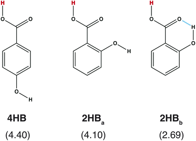 | ||
| Scheme 1 Chemical structures of hydroxybenzoic acid (HB) and pKa values computed with a quantum chemical approach8 in parentheses. | ||
Overcorrelation is another critical point in GNN and GCN studies. The overcorrelation in features indicates that they have irrelevant or redundant information.2,3 Jin et al. discussed the GNN performance based on feature overcorrelation. Their model (DeCorr) reduced feature correlation and performed better than the standard GNN approaches.3 Feature correlation in the convolution step was also focused on the GCN. It was shown that the GCN shows the degradation of the performance when the correlation of the features between the layers becomes large.9,10 Thus, the overcorrelation in the features should be removed in molecular GNNs.
Accuracy and overcorrelation are important points in feature selection. However, in chemistry, interpretability is considered more seriously. Recently, due to the development of theoretical methods and computers, various molecular properties can be computed accurately. However, to understand the chemistry, the reasons behind such physical properties must be investigated. In the quantum chemical field, an analysis of partial charges on the atoms, such as Mulliken and natural population analyses,11,12 is often applied. If the atomic charges are assigned to each atomic site, the chemists can image the charge flow in a molecule, which leads to the design of new molecules. Therefore, when molecular GNNs and GCNs are applied to chemistry, the obtained results should be explained with the employed features.
In this study, we propose a new feature for molecular GNNs considering accuracy, overcorrelation, and interpretability. In previous studies, most of descriptors employed in chemistry were molecular properties13,14 or isolated atomic properties15,16 or both,17,18 while molecular atomic properties computed with quantum chemical approaches were employed in this study. Although the preparation of the molecular atomic properties computed with quantum chemical calculations requires computational time, we can employ variety of atomic properties as descriptors, such as atomic charges, Fukui function,19 dispersion coefficients,20,21 isotropic magnetic shielding constant, and so on, which will be useful for better prediction. In the preparation of feature vectors from the molecular atomic properties, to improve the overcorrelation in GNNs, we employed the concatenation approach. Moreover, by coupling the integrated gradient approach with our model, the interpretability can be discussed based on the atomic site, which is useful in the design of molecules. Here, we evaluate the performance of the proposed model by computing the pKa values.
Method
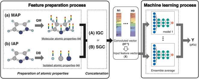
In this study, we proposed a new feature preparation process and constructed a machine learning (ML) process using the prepared features. Scheme 2 summarizes the flowchart of the present model. The feature preparation process comprises the preparation of atomic properties and concatenation. This section explains each step in detail.Preparation of atom properties
Various atom features have been applied in GCN studies.22,23 For example, Choudhary and DeCost employed the following eight atomic features in their GNN study: electronegativity, group number, covalent radius, valence electrons, first ionization energy, electron affinity, block, and atomic volume.23 They are isolated atomic properties (IAPs) and can be prepared without molecular information. In the quantum mechanical (QM) field, molecular-atomic properties (MAPs) are also employed for the analysis. After the QM calculations, various atomic properties are assigned to each atomic site using decomposition approaches.12,20,24,25In this study, we used the IAPs and the MAPs in feature preparation. In IAPs, the following six atomic properties were applied: effective nuclear charge, atomic polarizability, atomic radius, ionization energy, electron affinity, and atomic mass. Concerning the MAPs, the following nine properties were used: the positive and negative values of the constrained spatial electron density distribution (cSED) charge (Q+ and Q−),25 the positive and negative values of the isotropic magnetic shielding constant (σ+ and σ−), the positive and negative values of the molecular electrostatic potential (MEP)26–28 change at the nucleus (M+ and M−), the positive value of the partial Fukui function (F−),19 volume (V), and atomic dispersion coefficient (C6).20,21 Although the partial Fukui function also takes positive and negative values, only the positive value is important. For MEP, the potential negatively increases as the atomic number increases. In order to remove the atomic number dependency of the MEP, the M+ and M− were computed by subtracting the MEP value computed in an isolated atom from the MEP value computed in a molecule.
Concatenation of atomic properties
To construct the ML features from the atom properties, the GNN was considered. The hidden feature of node v in the l-th layer is denoted by h(l)v and h(0)v = xv, where x represents the node features (MAPs or IAPs). Moreover, h(l) is formally given along the update step, as follows:| h(l) = U(l)(h(l−1)), | (1) |
| H(L) ≡ h(0) ⊕ h(1) ⊕⋯⊕ h(L) | (2) |
Many processes in the update step are given in eqn (1). Concerning the simple graph convolution (SGC),31 the update step is given as follows:
| h(l) = Sh(l−1) = Slx | (3) |
![[D with combining tilde]](https://www.rsc.org/images/entities/b_char_0044_0303.gif) − 1/2Ã
− 1/2Ã![[D with combining tilde]](https://www.rsc.org/images/entities/b_char_0044_0303.gif) − 1/2, Ã = A + I, A is the adjacency matrix, and
− 1/2, Ã = A + I, A is the adjacency matrix, and ![[D with combining tilde]](https://www.rsc.org/images/entities/b_char_0044_0303.gif) is the degree matrix of Ã. Although the update step with S is well employed, it is known that the elements of Sl converge to a fixed value when l is large.32 To overcome this problem, the following update step was proposed:
is the degree matrix of Ã. Although the update step with S is well employed, it is known that the elements of Sl converge to a fixed value when l is large.32 To overcome this problem, the following update step was proposed:| h(l) = a(l)x | (4) |
 | (5) |
 | (6) |
![[b with combining macron]](https://www.rsc.org/images/entities/b_char_0062_0304.gif) is defined as follows:
is defined as follows:![[b with combining macron]](https://www.rsc.org/images/entities/b_char_0062_0304.gif) = D−1/2bD−1/2 = D−1/2bD−1/2 | (7) |
The employed atomic properties are defined with different units, and the maximum values in the properties differ. To remove the bias, we employed min–max normalization to H(L). The element h(l)i (0 ≤ l ≤ L) in H(L) was normalized with
 | (8) |
ML process
To discuss the performance of the prepared features, the supervised learning algorithm for pKa recognition was employed. The feature vector H(L) of the dissociated proton is chosen as an input vector X(0) in the multilayer perceptron (Scheme 2). The output Y (pKa in this study) is obtained as follows:| X(m) = σ(X(m−1)Θ(m) + β(m)), | (9) |
| Y = X(M−1)Θ(M) + β(M), | (10) |
Y depends on the weight and the hyperparameters, such as the number of nodes in the hidden layers and the dropout ratio. If the weight is optimized with different hyperparameters, different trained networks are produced. A linear combination of the corresponding outputs was taken as follows:34,35
 | (11) |
Computational details
Datasets
The pKa values and molecular information were obtained from the training and test sets prepared in the previous study.36 The number of molecules in the training and test sets are 2216 and 740, respectively. The datasets employed in this study were carefully cleaned and curated from the training and test sets by adopting the following steps. First, the molecules that have a CAS registry number were selected from the training and test sets. Next, we remove the molecules from the datasets when the pKa values are far from those of the analog or the deprotonation site is not clearly identified. In addition, the calculation was restricted to molecules with no iodide atom because of the current program limitation. Finally, 1014 and 316 pKa values were obtained for the training and test sets, respectively. The training datasets (1014 pKa values) were divided into training and validation datasets with a 80![[thin space (1/6-em)]](https://www.rsc.org/images/entities/char_2009.gif) :
:![[thin space (1/6-em)]](https://www.rsc.org/images/entities/char_2009.gif) 20 ratio (811 and 203 pKa values, respectively).
20 ratio (811 and 203 pKa values, respectively).
Hyperparameters
There are three layers, and the hidden size of the layers is n0, n1, and n0, respectively, which are summarized in Fig. S1 (ESI†). A hyperparameter search for the optimal hidden size (n0 and n1) and the dropout rate was computed using Optuna,37 where the Bayesian hyperparameter optimization was employed. The number of trial steps and epochs were 100 and 3000 epochs, respectively. The weight was further trained to 8000 epochs to improve its final accuracy.Calculations of molecules
The molecular geometries were computed at the CAM-B3LYP/aug-cc-pVDZ level of theory.38,39 The cSED charge, partial Fukui function, volume, atomic C6 dispersion coefficient, and MEP were computed using the GAMESS program package,40 and isotropic magnetic shielding constants on an atom were computed using the Gaussian program package.41The MAPs were also computed at the Hartree–Fock (HF)/6-31G** level of theory. Although a large difference in computational cost exists between HF/6-31G** and CAM-B3LYP/aug-cc-pVDZ, the difference in the predicted pKa was small, as shown in Fig. S2 (ESI†).
Results and discussion
The correlation between features was evaluated using Pearson's correlation coefficient, | (12) |
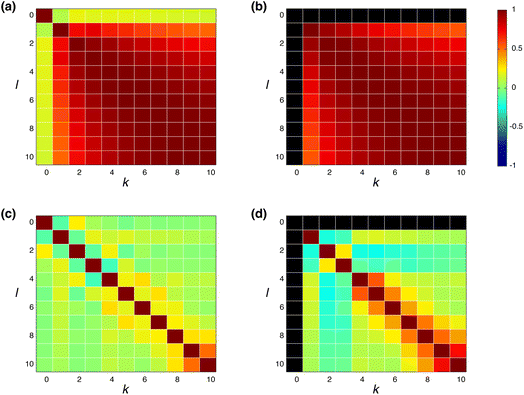
![[h with combining macron]](https://www.rsc.org/images/entities/b_char_0068_0304.gif) (k) is the mean value of h(k)i. The input feature of molecule i was prepared by taking the concatenation of {h(k)i} (eqn (2) and Scheme 2). A large ρk,l means that h(k)i and h(l)i are similar and they have common information, while a small ρk,l means that h(k)i and h(l)i have unique information and their overlap became small. When the common features among h(k)i and h(l)i are repeated in the concatenation (eqn (2)), the concatenated vector H(L) and input vector X(0) contain the redundant data.42 In Fig. 1, the heat maps of ρk,l computed with IGC and SGC are shown. In the correlation calculations, IAPs and MAPs were employed as the atomic properties. Because h(0)i computed with IAPs have the same values among the molecules, the correlation coefficients (ρ0,l and ρk,0) cannot be defined, which were colored black in Fig. 1. As shown in Fig. 1(a), the correlation between h(0) and h(k) (k ≥ 1) was small in the case of SGC(MAP), whereas the correlations between h(k) and h(l) (k, l ≥ 1) were large in both cases of MAPs and IAPs (Fig. 1(a) and (b)). Therefore, the redundancy in the features of constructed X(0) should be large when SGC(IAP) is employed. By contrast, the correlation between the x-th and y-th layer vectors is small when IGC is chosen (Fig. 1(c) and (d)). From the results, we concluded that the redundancy in the X(0) constructed with IGC should be reduced.
(k) is the mean value of h(k)i. The input feature of molecule i was prepared by taking the concatenation of {h(k)i} (eqn (2) and Scheme 2). A large ρk,l means that h(k)i and h(l)i are similar and they have common information, while a small ρk,l means that h(k)i and h(l)i have unique information and their overlap became small. When the common features among h(k)i and h(l)i are repeated in the concatenation (eqn (2)), the concatenated vector H(L) and input vector X(0) contain the redundant data.42 In Fig. 1, the heat maps of ρk,l computed with IGC and SGC are shown. In the correlation calculations, IAPs and MAPs were employed as the atomic properties. Because h(0)i computed with IAPs have the same values among the molecules, the correlation coefficients (ρ0,l and ρk,0) cannot be defined, which were colored black in Fig. 1. As shown in Fig. 1(a), the correlation between h(0) and h(k) (k ≥ 1) was small in the case of SGC(MAP), whereas the correlations between h(k) and h(l) (k, l ≥ 1) were large in both cases of MAPs and IAPs (Fig. 1(a) and (b)). Therefore, the redundancy in the features of constructed X(0) should be large when SGC(IAP) is employed. By contrast, the correlation between the x-th and y-th layer vectors is small when IGC is chosen (Fig. 1(c) and (d)). From the results, we concluded that the redundancy in the X(0) constructed with IGC should be reduced.
It is useful to consider the meaning of the small correlation between h(k) and h(l) (k ≠ l) in IGC(MAP) based on spectral filtering. When vi and λi are the i-th eigenvector and eigenvalue of Laplacian, respectively, the spectral filtering on graph signal x can be written as follows:
 | (13) |
| y(k) ≡ f(λk)vkvTkx | (14) |
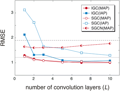
The redundancy in the feature vector X(0) probably affects the accuracy of the predicted pKa values. To discuss the relationship between the accuracy and the redundancy in X(0), the root mean square errors (RMSEs) of the pKa values were calculated. Because X(0) is the concatenated vector H(L) of the dissociated proton, the size of X(0) is controlled by the convolution layers (L). In Fig. 2, the RMSEs computed with L = 1, 2, 3, 5, 7, and 10 are shown. For comparison, the RMSEs were also computed with a freely available pKa prediction tool called OPERA36 and MolGpKa.44 In the case of MolGpKa, the model was optimized using the dataset employed in this study. To evaluate the effectiveness of the concatenation in eqn (2), we performed an ablation study about SGC without the concatenated module. In the ablation study, SLx was employed as the feature vector X(0), which is the analogue of a simplified graph neural network (SGCN).31 When an IAP was employed, there was a large difference in the accuracy between the convolution approaches, SGC and IGC. Although the error in IGC(IAP) and SGC(IAP) decreases as L increases, the error in IGC(IAP) is largely improved as L increases when compared with that in SGC(IAP). This is because the redundancy in X(0) of IGC(IAP) is smaller than that of SGC(IAP) (Fig. 1). When a MAP was employed, the RMSE is small in both cases of IGC and SGC because X(0) has unique information even with a small L value (Fig. 1(a) and (c)). In both cases of SGC and IGC with a concatenated module, the prediction performance was improved up to L = 10, while the SGCN model with MAPs gave the best performance with L = 2. This difference shows that the concatenation in eqn (2) plays an important role in accurate prediction.
Although the RMSE shown in Fig. 2 is one of the good properties to discuss accuracy, it is also important to check whether the prepared features can reproduce the pKa difference stemming from the structural difference (Scheme 1). In Table 1, the pKa values of hydroxybenzoic acids predicted with IGC(MAP), IGC(IAP), SGC(MAP), SGC(IAP), MolGpKa, and OPERA are shown. As a reference, the pKa values computed with QM approaches are also shown.8 The obtained pKa values reproduced the pKa values computed with the QM, except for MolGpKa. Moreover, IGC(MAP), SGC(IAP), and OPERA can reproduce the QM result where the pKa of 4HB is larger than that of 2HB, suggesting that SGC and IGC can include structural isomerism through convolution. However, the pKa difference between 2HBa and 2HBb was reproduced only with IGC(MAP), IGC(IAP), and SGC(MAP). The results show that the IGC(MAP) gave a good feature to reproduce the pKa difference stemming from the structural difference.
| IGC(MAP) | IGC(IAP) | SGC(MAP) | SGC(IAP) | MolGpKa | OPERA | QM | |
|---|---|---|---|---|---|---|---|
| 4HB | 3.58 | 4.00 | 3.46 | 3.93 | 7.61 | 4.47 | 4.40 |
| 2HBa | 3.23 | 4.10 | 3.47 | 3.42 | 7.88 | 3.53 | 4.10 |
| 2HBb | 1.71 | 3.97 | 2.49 | 3.42 | 7.88 | 3.53 | 2.69 |
From the viewpoint of accuracy and the correlation between features, IGC with MAPs is superior to others. However, with accuracy, it is difficult to say if the concatenated vector computed with IGC(MAP) is a good feature. To discuss the interpretability of the IGC(MAP), the integrated gradients (IGs) were computed.
 | (15) |
![[X with combining macron]](https://www.rsc.org/images/entities/b_char_0058_0304.gif) (0) is the baseline. Although it is well known that the baseline is important in calculating IGs, there is no universal rule to define the baseline. It is also difficult to determine the baseline of pKa. As shown in a previous study,36 most of the DataWarrior acidic pKa values, which are a freely available pKa dataset,45 are within the range (0 < pKa < 14). Therefore, the middle of the pKa range (pKa = 7) is a candidate for the baseline. In this study, the H-value of 4-nitrophenol was chosen as the baseline
(0) is the baseline. Although it is well known that the baseline is important in calculating IGs, there is no universal rule to define the baseline. It is also difficult to determine the baseline of pKa. As shown in a previous study,36 most of the DataWarrior acidic pKa values, which are a freely available pKa dataset,45 are within the range (0 < pKa < 14). Therefore, the middle of the pKa range (pKa = 7) is a candidate for the baseline. In this study, the H-value of 4-nitrophenol was chosen as the baseline ![[X with combining macron]](https://www.rsc.org/images/entities/b_char_0058_0304.gif) (0) in eqn (15) because the pKa value is close to 7. With this baseline, we can say that the positive IGi suggests that the i-th feature contributes to less acidic character (pKa > 7) and the negative IGi suggests that the i-th feature contributes to more acidic character (pKa < 7).
(0) in eqn (15) because the pKa value is close to 7. With this baseline, we can say that the positive IGi suggests that the i-th feature contributes to less acidic character (pKa > 7) and the negative IGi suggests that the i-th feature contributes to more acidic character (pKa < 7).
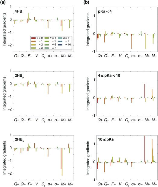
Fig. 3(a) summarizes the IGs of 4HB, 2HBa, and 2HBb computed with the baseline. Because the pKa values of 4HB, 2HBa, and 2HBb are <7, the negative IGs are important. Fig. 3(a) shows that the difference among the molecules mainly comes from the properties, M+ (k = 0) and M+ (k = 2), where M+ is the positive MEP value. Previous studies27,28 have shown that the MEP had a strong negative correlation with the sum of valence natural atomic orbital energies. Therefore, the IGs in Fig. 3(a) show that the pKa value decreases as the atomic orbital energy becomes increasingly negative. Because the electron-withdrawing atom makes the atomic orbital energy of the next atom more negative, the IGs in Fig. 3(a) also indicate that the pKa value decreases when the sites of k = 0 and 2 are surrounded by the more electron-withdrawing atoms.
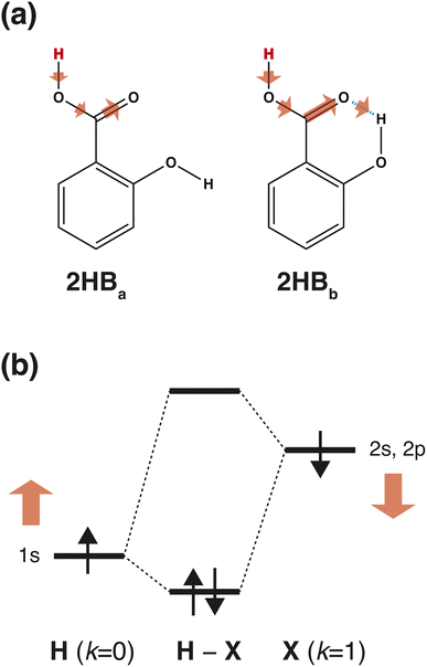
As shown in Scheme 3(a), in the case of 2HBa, and 2HBb, the sites of k = 0 and 2 are the proton H and carbonyl C sites, respectively. When the chemical structure is considered, the carbonyl O atom of 2HBb can withdraw the electron on the carbonyl C atom more strongly than that of 2HBa. From the pKa difference between 2HBa and 2HBb, and Scheme 3(a), the explanation by IGs is reasonable.
Although the interpretation in Scheme 3(a) is reasonable for an acidic compound (2HB), checking the interpretation along the pKa value is also important. To discuss the interpretation change, the average of IGs in the three pKa ranges (pKa < 4, 4 ≤ pKa < 10, and 10 ≤ pKa) was obtained. In Fig. 3(b), the averaged IGs are shown. Although the averaged IGs in the range pKa < 4 are similar to those in Fig. 3(a), the averaged IGs in the range 10 ≤ pKa differ totally from those in Fig. 3(a). Under weak acid conditions (10 ≤ pKa), the IGs of M+ (k = 0) and M− (k = 1) are positively large. The obtained IG is reasonable because of the following reasons. When the M+ and M− values increase, the orbital energy difference decreases (Scheme 3(b)), and the polarity of the bond decreases. The large positive IG suggests that the low polarity in the chemical bond makes the pKa value positive (less acidic), which is reasonable from the chemical viewpoint, if the size effect is omitted. Scheme 3 shows that the ML model obtained with IGC(MAP) gives a reasonable interpretation for chemists.
Conclusions
In this study, a new feature in molecular GNNs was proposed, and the accuracy, overcorrelation between features, and interpretability were discussed in detail. The overcorrelation and accuracy indicate that the IGC with MAPs is superior to others. The prediction output with the IGC(MAP) was analyzed using the IG method. From the analysis, positive values of MEP (k = 0 and 2) are important under acidic conditions, whereas the positive value of MEP (k = 0) and the negative value of MEP (k = 1) are important under basic conditions, which leads to a reasonable interpretation from a chemistry viewpoint.In this study, a part of the concatenated vectors {H(L)} was employed in the ML model. In the future study, we will employ all {H(L)} in a molecule to construct the ML model for predicting molecular properties, such as the solvation free energy and octanol/water partition coefficient.
Data availability
The program to predict pKa from the concatenated vector H(L) is available as open access via GitHub (https://github.com/dyokogawa/pKa_prediction). The training, validation, and test sets used in this paper were also included in the repository (Opt1_acidic_tr.csv and Opt1_acidic_tst.csv).Author contributions
D. Y. developed the theoretical formalism and the programs and performed the predictions. D. Y. and K. S. performed the quantum chemical calculations for the preparation of atomic features using CAM-B3LYP/aug-cc-pVDZ and HF/6-31G**, respectively. Both authors contributed to the final version of the manuscript.Conflicts of interest
There are no conflicts to declare.Acknowledgements
This study was supported by JST, PRESTO Grant Number JPMJPR21C9, and the Leading Initiative for Excellent Young Researchers. We also acknowledge Enago (https://www.enago.jp) for the English language review.References
- A.-C. Haury, P. Gestraud and J.-P. Vert, The Influence of Feature Selection Methods on Accuracy, Stability and Interpretability of Molecular Signatures, PLoS One, 2011, 6, e28210 CrossRef CAS PubMed.
- D. B. Acharya and H. Zhang, Feature Selection and Extraction for Graph Neural Networks, in Proceedings of the 2020 ACM Southeast Conference, 2019, pp. 252–255 Search PubMed.
- W. Jin, X. Liu, Y. Ma, C. Aggarwal and J. Tang, Feature Overcorrelation in Deep Graph Neural Networks, Proceedings of the 28th ACM SIGKDD Conference on Knowledge Discovery and Data Mining, 2022 Search PubMed.
- S. Ishida, K. Terayama, R. Kojima, K. Takasu and Y. Okuno, Prediction and Interpretable Visualization of Retrosynthetic Reactions Using Graph Convolutional Networks, J. Chem. Inf. Model., 2019, 59, 5026–5033 CrossRef CAS PubMed.
- R. Kojima, S. Ishida, M. Ohta, H. Iwata, T. Honma and Y. Okuno, kGCN: a graph-based deep learning framework for chemical structures, J. Cheminf., 2020, 12, 32 CAS.
- M. Jiang, Z. Li, S. Zhang, S. Wang, X. Wang, Q. Yuan and Z. Wei, Drug-target affinity prediction using graph neural network and contact maps, RSC Adv., 2020, 10, 20701–20712 RSC.
- A. Kensert, R. Bouwmeester, K. Efthymiadis, P. Van Broeck, G. Desmet and D. Cabooter, Graph Convolutional Networks for Improved Prediction and Interpretability of Chromatographic Retention Data, Anal. Chem., 2021, 93, 15633–15641 CrossRef CAS PubMed.
- T. Baba, T. Matsui, K. Kamiya, M. Nakano and Y. Shigeta, A density functional study on the pKa of small polyprotic molecules, Int. J. Quantum Chem., 2014, 114, 1128–1134 CrossRef CAS.
- Q. Li, Z. Han, X.-M. Wu, Deeper Insights into Graph Convolutional Networks for Semi-Supervised Learning, in Proceedings of the Thirty-Second AAI Conference on Artificial Intelligence, 2018, pp. 3538–3545 Search PubMed.
- M. Chen, Z. Wei, Z. Huang, B. Ding and Y. Li, Simple and Deep Graph Convolutional Networks, Proceedings of the 37th International Conference on Machine Learning, 2020, pp. 1725–1735 Search PubMed.
- R. S. Mulliken, Electronic population analysis on LCAO-MO molecular wave functions. I, J. Chem. Phys., 1955, 23, 1833–1840 CrossRef CAS.
- A. E. Reed, R. B. Weinstock and F. Weinhold, Natural population analysis, J. Chem. Phys., 1985, 83, 735–746 CrossRef CAS.
- B. Huang and O. A. von Lilienfeld, Communication: Understanding molecular representations in machine learning: The role of uniqueness and target similarity, J. Chem. Phys., 2016, 145, 161102 CrossRef PubMed.
- F. Pereira, K. Xiao, D. A. R. S. Latino, C. Wu, Q. Zhang and J. Aires-de Sousa, Machine Learning Methods to Predict Density Functional Theory B3LYP Energies of HOMO and LUMO Orbitals, J. Chem. Inf. Model., 2017, 57, 11–21 CrossRef CAS PubMed.
- J. P. Janet and H. J. Kulik, Resolving Transition Metal Chemical Space: Feature Selection for Machine Learning and Structure–Property Relationships, J. Phys. Chem. A, 2017, 121, 8939–8954 CrossRef CAS PubMed.
- K. T. Schütt, M. Gastegger, A. Tkatchenko, K. R. Müller and R. J. Maurer, Unifying machine learning and quantum chemistry with a deep neural network for molecular wavefunctions, Nat. Commun., 2019, 10, 5024 CrossRef PubMed.
- Y. Zhuo, A. Mansouri Tehrani and J. Brgoch, Predicting the Band Gaps of Inorganic Solids by Machine Learning, J. Phys. Chem. Lett., 2018, 9, 1668–1673 CrossRef CAS PubMed.
- J. Jiménez-Luna, M. Skalic, N. Weskamp and G. Schneider, Coloring Molecules with Explainable Artificial Intelligence for Preclinical Relevance Assessment, J. Chem. Inf. Model., 2021, 61, 1083–1094 CrossRef PubMed.
- F. Jensen, Introduction to Computational Chemistry, John Wiley and Sons, Chichester, 2nd edn, 2006 Search PubMed.
- D. Yokogawa, Isotropic Site-Site Dispersion Potential Constructed Using QuantumChemical Calculations and a Geminal Auxiliary Basis Set, Bull. Chem. Soc. Jpn., 2019, 92, 748–753 CrossRef CAS.
- D. Yokogawa, Isotropic Site-Site Dispersion Potential Determined from Localized Frequency-Dependent Density Susceptibility, Bull. Chem. Soc. Jpn., 2019, 92, 1694–1700 CrossRef CAS.
- B. Ramsundar, P. Eastman, P. Walters, V. Pande, K. Leswing and Z. Wu, Deep Learning for the Life Sciences, O'Reilly Media, 2019, https://www.amazon.com/Deep-Learning-Life-Sciences-Microscopy/dp/1492039837 Search PubMed.
- K. Choudhary and B. DeCost, Atomistic Line Graph Neural Network for improved materials property predictions, npj Comput. Mater., 2021, 7, 185 CrossRef.
- R. F. W. Bader, A quantum theory of molecular structure and its applications, Chem. Rev., 1991, 91, 893–928 CrossRef CAS.
- D. Yokogawa and K. Suda, Electrostatic Potential Fitting Method Using Constrained Spatial Electron Density Expanded with Preorthogonal Natural Atomic Orbitals, J. Phys. Chem. A, 2020, 124, 9665–9673 CrossRef CAS PubMed.
- P. Politzer, P. R. Laurence and K. Jayasuriya, Molecular electrostatic potentials: an effective tool for the elucidation of biochemical phenomena, Environ. Health Perspect., 1985, 61, 191–202 CrossRef CAS PubMed.
- S. Liu, C. K. Schauer and L. G. Pedersen, Molecular acidity: A quantitative conceptual density functional theory description, J. Chem. Phys., 2009, 131, 164107 CrossRef PubMed.
- S. Liu and L. G. Pedersen, Estimation of Molecular Acidity via Electrostatic Potential at the Nucleus and Valence Natural Atomic Orbitals, J. Phys. Chem. A, 2009, 113, 3648–3655 CrossRef CAS PubMed.
- J. F. Lutzeyer, C. Wu, M. Vazirgiannis, Sparsifying the Update Step in Graph Neural Networks, Proceedings of Topological, Algebraic and Geometric Learning Workshops, 2022, pp. 258–268 Search PubMed.
- K. Xu, C. Li, Y. Tian, T. Sonobe, K.-i. Kawarabayashi, and S. Jegelka, Representation Learning on Graphs with Jumping Knowledge Networks, Proceedings of the Thirty-Fifth International Conference on Machine Learning, 2018, pp. 5453–5462 Search PubMed.
- F. Wu, T. Zhang, A. H. d. Souza, C. Fifty, T. Yu, and K. Q. Weinberger, Simplifying Graph Convolutional Networks, Proceedings of the Thirty-Sixth International Conference on Machine Learning, 2019, pp. 6861–6871 Search PubMed.
- X. Liu, F. Lei, G. Xia, Y. Zhang and W. Wei, AdjMix: simplifying and attending graph convolutional networks, Complex Intell. Syst., 2022, 8, 1005–1014 CrossRef.
- K. B. Wiberg, Application of the Pople-Santry-Segal CNDO method to the cyclopropylcarbinyl and cyclobutyl cation and to bicyclobutane, Tetrahedron, 1968, 24, 1083–1096 CrossRef CAS.
- S. Hashem and B. Schmeiser, Improving model accuracy using optimal linear combinations of trained neural networks, IEEE Trans. Neural Networks, 1995, 6, 792–794 CrossRef CAS PubMed.
- S. Hashem, Optimal Linear Combinations of Neural Networks, Neural Networks, 1997, 10, 599–614 CrossRef PubMed.
- K. Mansouri, N. F. Cariello, A. Korotcov, V. Tkachenko, C. M. Grulke, C. S. Sprankle, D. Allen, W. M. Casey, N. C. Kleinstreuer and A. J. Williams, Open-source QSAR models for pKa prediction using multiple machine learning approaches, J. Cheminf., 2019, 11, 60 Search PubMed.
- T. Akiba, S. Sano, T. Yanase, T. Ohta and M. Koyama, Optuna: A Next-generation Hyperparameter Optimization Framework, Proceedings of the 25th ACM SIGKDD International Conference on Knowledge Discovery and Data Mining, 2019 Search PubMed.
- T. Yanai, D. P. Tew and N. C. Handy, A new hybrid exchange-correlation functional using the Coulomb-attenuating method (CAM-B3LYP), Chem. Phys. Lett., 2004, 393, 51–57 CrossRef CAS.
- R. A. Kendall, T. H. Dunning Jr and R. J. Harrison, Electron affinities of the first-row atoms revisited. Systematic basis sets and wave functions, J. Chem. Phys., 1992, 96, 6796–6806 CrossRef CAS.
- M. W. Schmidt, K. K. Baldridge, J. A. Boatz, S. T. Elbert, M. S. Gordon, J. H. Jensen, S. Koseki, N. Matsunaga, K. A. Nguyen, S. Su, T. L. Windus, M. Dupuis and J. A. Montgomery, General atomic and molecular electronic structure system, J. Comput. Chem., 1993, 14, 1347–1363 CrossRef CAS.
- M. J. Frisch, et al., Gaussian 16 Revision A.03, Gaussian Inc., Wallingford CT, 2016 Search PubMed.
- K. Zhang, Z. Li, F. Zhang, W. Wan and J. Sun, Pan-Sharpening Based on Transformer With Redundancy Reduction, IEEE Geosci. Rem. Sens. Lett., 2022, 19, 1–5 Search PubMed.
- F. Opolka, Y.-C. Zhi, P. Lió and X. Dong, Adaptive Gaussian Processes on Graphs via Spectral Graph Wavelets, Proceedings of The 25th International Conference on Artificial Intelligence and Statistics, 2022, pp. 4818–4834 Search PubMed.
- X. Pan, H. Wang, C. Li, J. Z. H. Zhang and C. Ji, MolGpka: A Web Server for Small Molecule pKa Prediction Using a Graph-Convolutional Neural Network, J. Chem. Inf. Model., 2021, 61, 3159–3165 CrossRef CAS PubMed.
- T. Sander, J. Freyss, M. von Korff and C. Rufener, DataWarrior: An Open-Source Program For Chemistry Aware Data Visualization And Analysis, J. Chem. Inf. Model., 2015, 55, 460–473 CrossRef CAS PubMed.
Footnote |
| † Electronic supplementary information (ESI) available: Details of the machine learning process, RMSEs of the pKa values obtained by IGC and two types of atom features (IAPs and MAPs), which were computed with the Hartree–Fock (HF)/6-31G** level of theory, and experimental and calculated pKa values of the test set. See DOI: https://doi.org/10.1039/d3dd00010a |
| This journal is © The Royal Society of Chemistry 2023 |

