Transfer learning on large datasets for the accurate prediction of material properties

Abstract

Graph neural networks trained on large crystal structure databases are extremely effective in replacing ab initio calculations in the discovery and characterization of materials. However, crystal structure datasets comprising millions of materials exist only for the Perdew–Burke–Ernzerhof (PBE) functional. In this work, we investigate the effectiveness of transfer learning to extend these models to other density functionals. We show that pre-training significantly reduces the size of the dataset required to achieve chemical accuracy and beyond. We also analyze in detail the relationship between the transfer-learning performance and the size of the datasets used for the initial training of the model and transfer learning. We confirm a linear dependence of the error on the size of the datasets on a log–log scale, with a similar slope for both training and the pre-training datasets. This shows that further increasing the size of the pre-training dataset, i.e., performing additional calculations with a low-cost functional, is also effective, through transfer learning, in improving machine-learning predictions with the quality of a more accurate, and possibly computationally more involved functional. Lastly, we compare the efficacy of interproperty and intraproperty transfer learning.

---

I. Introduction

Over the past decade, machine learning models have emerged as unbeatable tools to accelerate materials research in fields ranging from quantum chemistry¹ to drug discovery² to solid-state materials science.^3–6 One of the major drivers of progress has been the transition from simpler models based on a single material family to more advanced and more universal models.^7–9 The current state of the art are graph neural networks and graph transformers.¹⁰ However, the accuracy of these complex models, which include millions of parameters, depends heavily on the amount and quality of the training data.¹¹ Consequently, the development of such models is conditional on the availability of large databases of calculations obtained with consistent computational parameters.

In quantum chemistry, there are a variety of large databases that gather calculations with varying degrees of accuracy, from density functional theory (with different functionals) to coupled-cluster.¹² In comparison, in solid-state materials science, all large databases (>10⁵ compounds) contain calculations performed using the Perdew–Burke–Ernzerhof (PBE) functional.¹³ The list includes AFLOW,¹⁴ the OQMD,^15,16 the Materials Project,¹⁷ and DCGAT.¹⁸ An exception is the smaller JARVIS database that encompasses ∼55 k calculations obtained using OptB88-vdW^19,20 and the modified Becke–Johnson potential.^21–23 The first large databases beyond the PBE functional have been published only recently.^24,25 These datasets are based on the PBE functional for solids (PBEsol),²⁶ the highly constrained and appropriately normalized semilocal functional (SCAN),²⁷ and the R2SCAN functional.²⁸ All of these density functionals yield much more accurate geometries than the PBE, and the latter two also yield more accurate formation energies and band gaps.^29–32 Nevertheless, these databases are one to two orders of magnitude smaller than the largest PBE databases.

Currently, graph networks^7,8,33–35 are the best performing models for datasets including more than 10⁴ compounds.¹¹ However, they improve dramatically with increasing dataset size beyond this number. Consequently, despite the higher accuracy of PBEsol or SCAN, models trained on these smaller datasets have a significantly larger prediction error compared to their PBE counterparts. One way to circumvent the problem of data sparsity is to perform transfer learning and pre-training, as these approaches have proved to be extremely effective in other fields.^36,37 In the areas of computer vision and natural language processing, for instance, almost all non-edge applications can be improved by using large pre-trained models.^36,37

In recent years, transfer learning and multi-fidelity learning have also arrived in materials science.^7,38–49 The published works deal with rather small datasets for both pre-training and transfer learning, usually ≲10⁴ data points for the transfer dataset and ≲10⁵ data points for the pre-training dataset. In this context, band gaps^7,38,46,48 and formation energies^39,48 are the most popular features for transfer learning, since there is abundance of multi-fidelity theoretical and experimental data (∼10³ measurements).

Hutchinson et al.³⁸ compare multi-task training, latent variables, and delta learning for small datasets finding mixed results for the best strategy depending on the dataset.

Very few applications have been made in the realm of big data, since hardly any large data sets exist. Smith et al.¹² improved ANI⁴⁰ quantum chemistry force fields beyond the accuracy of DFT by transferring from the ANI-1x DFT dataset that contains 5.2 million molecules to a dataset of 0.5 million molecules computed with coupled cluster.¹² They explored both transfer learning by retraining the last layers of their neural network as well as delta learning by first predicting DFT energies and then the difference from DFT to coupled cluster with a second network. Both approaches markedly outperformed naive direct training on coupled cluster data, with the delta learning approach achieving 1% smaller errors than transfer learning.

Kolluru et al.⁴⁵ used a model pre-trained on the Open Catalyst Dataset OC20 (ref. 50) to obtain better results on the smaller MD17 dataset⁵¹ as well as on other open catalyst datasets. They studied the retraining of various layers as well as the addition of extra randomly initialized layers and attention based weighting of pre-trained embeddings. For the in-domain dataset they found that embeddings from deeper interaction layers were more relevant while for out of domain data the attention based combination of embeddings from different depth was required. In this work, we investigate the benefits of transfer learning when large materials datasets are available, investigating both cross-property transfer and prediction improvement through high-accuracy data. We will compare retraining of the whole graph networks and transfer learning with a fixed graph embedding network.

We focus mainly on properties that are important for the discovery of new crystal structures. In this context, the energy distance to the convex hull of thermodynamic stability is a key quantity, as it compares the formation energy of a crystalline compound with the combined energy of the available decomposition channels. In ref. 24 we have published a data set with 175 k SCAN²⁷ total energies and PBEsol²⁶ geometries of stable and metastable systems. In preparation of this work, we have extended that dataset to include additional ∼50 k calculations of randomly selected unstable systems with a distance from the convex hull of thermodynamic stability below 800 meV per atom. Calculations using SCAN show about half the mean absolute error (MAE) for formation energies compared to calculations with the standard PBE functional.³² Similarly, calculations using PBEsol reduce the mean absolute percent errors on volumes by 40% compared to PBE.³⁰

In the following, we will demonstrate that pre-training using a large PBE dataset allows us to obtain improved predictions, with the accuracy of more advanced density functionals, even when the available training data is limited for the latter. Furthermore, we will evaluate the dependence of the error on the size of the training and pre-training data to quantify potential gains through future expansion of the datasets of calculations. We also investigate to which extent transfer learning is useful to improve predictions of different materials properties.

II. Results

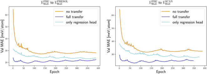
We started our transfer learning experiments by training crystal graph-attention neural networks³⁵ on a PBE dataset with 1.8 M structures¹⁸ from the DCGAT database, and on the extended PBEsol and SCAN datasets from ref. 24. The DCGAT dataset combines compatible data from AFLOW,¹⁴ the materials project¹⁷ and ref. 18, 35 and 52–54. We generally used a train/val/test split of 80/10/10%. The same training, validation and test set were randomly selected once for PBEsol and SCAN and then kept constant for all experiments to ensure a fair comparison. As a starting point, one model was trained for each of the three functionals and for four properties, specifically the distance to the convex hull (E_hull), the formation energy (E_form), the band gap and the volume per atom of the unit cell. For the band gaps only PBE and SCAN models were trained, as PBEsol and PBE band gaps are very similar, and we did not perform transfer learning for SCAN volumes as we only have calculated PBE and PBEsol geometries.

The initial neural network, trained on the PBE datasets comprising 1.8 M calculations, predicts the distance to the convex hull of the systems in the test set with a MAE of 23 meV per atom. As expected, the same neural networks, trained from scratch using significantly smaller PBEsol and SCAN datasets (this procedure is labelled “no transfer” in the figures and tables), perform worse and yield, respectively, 9% and 23% higher MAEs. To take advantage of transfer learning we considered two options: starting from the neural network trained with the large PBE dataset, we either continue the training of the whole network with the PBEsol or the SCAN data (this procedure is denoted “full transfer”), or we fix most of the weights and train only the residual network that follows the message passing part, i.e., the one that calculates the scalar output from the final graph embedding (this procedure is indicated as “only regression head”). Comparing in Fig. 1 and Table 1 these two approaches of transfer learning to the original model trained solely on the smaller datasets, we can immediately conclude that, in all cases, transfer learning enhances considerably the performance of the neural network.

Fig. 1 Learning curves, i.e., MAE on the validation set as a function of the training epoch, for the prediction of E^PBEsol_hull (left) and E^SCAN_hull (right) using the different training procedures, without pre-training (no transfer), with pre-training using E^PBE_hull data and freezing part of the weights (only regression head) and with pre-training using E^PBE_hull data and successive full reoptimization of all weights (full transfer). We employed a triangular learning rate schedule, in which the learning rate oscillated between a minimum of 0.1 times and a maximum of the original learning rate. This results in the cyclical behavior in the training plots.

Table 1 Intra-property transfer learning. We report the mean absolute errors on the test set for the neural networks trained on the large PBE dataset only and the neural networks trained on the PBEsol and SCAN datasets with and without transfer learning. The different approaches for transfer learning (only regression head and full transfer) are explained in the text. The models with the best performance for PBEsol/SCAN are indicated with bold letters. The percent improvement in comparison to the case of no transfer learning are shown in parenthesis

	PBE	PBEsol			SCAN
		No transfer	Only regression head	Full transfer	No transfer	Only regression head	Full transfer
E hull [meV per atom]	23	26	22 (15%)	19 (27%)	31	26 (16%)	22 (29%)
E form [meV per atom]	18	20	18 (10%)	13 (35%)	24	22 (8%)	16 (33%)
Volume [Å^3 per atoms]	0.24	0.21	0.18 (14%)	0.16 (23%)
Band gap [eV]	0.020				0.078	0.93 (−19%)	0.068 (13%)

---

Applying the neural network trained on the PBE data, after retraining only the output network on the PBEsol/SCAN dataset, resulted in improved predictions in comparison to the ones of the same network trained only on the PBEsol/SCAN dataset. This type of transfer learning leads to a 15% smaller test MAE for the PBEsol data and 16% smaller test MAE for the SCAN data. Retraining the full network resulted in an even better performance, with a reduction of the MAE on the test set, after only ∼70 epochs, by 27% and 29% for the PBEsol and SCAN data, respectively.

If we use the same neural network to predict the formation energy instead of the distance to the convex hull, the results are very similar, as shown in Table 1. Transfer learning with retraining of the output network leads in this case to an error reduction of 10% and 8% for PBEsol and SCAN, respectively. On the other hand, extending the training of the full network to the additional datasets brings an even higher error reduction of 35 and 33% for PBEsol and SCAN, respectively. Again both transfer learning approaches give consistently a lower MAE than the neural network trained anew on smaller datasets, demonstrating the benefit of exploiting the larger database of less accurate, but computationally more affordable, PBE calculations.

The visible discrepancies in the performance of the fully retrained network and the partially retrained network, where only the weights of the output network are further optimized, hint to the fact that the crystal graph embeddings for the three functionals must differ significantly.

We only have available PBEsol volumes, as the data was generated with the approach of ref. 24. Consequently, we only test the transfer learning for the PBEsol functional achieving an improvement of 23%.

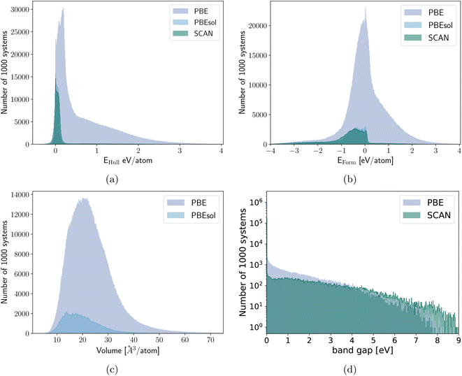
The band gaps are the sole material property where we only obtain an improvement (with a 13% MAE reduction) when the training on the new data is performed for the whole network. We have to be careful in considering the MAE for this dataset as most of the materials are metals with a band gap equal to zero. If the machine predicts zero band gap, i.e., a metal, the associated error on the band gap value will be zero for a metal, while a finite error can be associated to the prediction of an open band gap. There are remarkable differences in the band gap distribution for calculations performed with the two different functionals (also visible in Fig. 2d), as PBE underestimates the band gap more strongly than SCAN. This results in an average band gap of 0.08 eV in the PBE dataset and of 0.47 eV in the SCAN dataset. The fact that PBE misclassifies some semiconductors as metals leads to an MAE artificially smaller for the machine trained on PBE data, as more metals are contained in the PBE dataset. While the distributions for other properties also differ, there is in this case a qualitative difference between metals and semiconductors and it is necessary that the network trained on the SCAN data also learns also how to distinguish false metals in the PBE dataset. The training of the regression head only is therefore totally insufficient. By training solely on semiconductors with band gaps larger than 0.1 eV, we observed an improvement of 9% for a full retraining of the PBE network for SCAN band gaps above the same cutoff. However, based on Fig. 3 and considering that the limits on the band gap resulted in a reduced transfer learning data set for this task, we expect that the transfer learning performance for band gaps larger than 0.1 eV aligns with that of other quantities.

Fig. 2 Histogram of (a) the distances to the convex hull and (b) the formation energies of the PBE, PBEsol and SCAN datasets. (c) Histogram of the volumes of the PBE and PBEsol dataset. (d) Histogram of the band gaps of the PBE and SCAN datasets.

Fig. 3 The left panel shows the log–log plot for the MAE on the test set for the prediction of E^SCAN_hull as a function of the training set size. We consider the cases of full transfer with pre-training datasets of different size (different shades of blue) or no transfer (orange). The right panel shows the same MAE as a function of the pre-training dataset, for different values of the training datasets (different shades of blue). In the insets we indicate the slopes and the y-intercepts according to the linear fit and the purple line marks “chemical accuracy”.

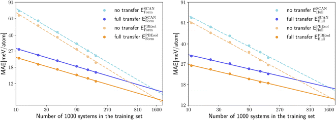
Now that we are convinced of the benefits of pre-training on a larger lower-quality dataset to speed up successive training on a higher-quality dataset, we can further inspect how the performance of transfer learning depends on the size of the training set. The log–log plots of Fig. 4 offer a clear insight into the quantity of high-quality data required in case of transfer from the pre-trained PBE model (with training of the full network on the new data) and no transfer. In the left panel of Fig. 4 we show the MAE for the prediction of SCAN and PBEsol energy distances to the convex hull E^SCAN/PBEsol_hull, while in the right panel of Fig. 4 the MAE for the prediction of SCAN and PBEsol formation energies E^SCAN/PBEsol_form is displayed. All models are again evaluated on the same test set. In both panels of Fig. 4 we observe that we reach chemical precision (i.e., an error below 43 meV per atom) already at 11 k training systems. We can therefore conclude that fitting neural networks to computationally expensive calculations based on hybrid or double-hybrid functionals will be enabled in the near future by transfer learning. We can easily fit the points in the log–log plots with lines and extrapolate the number of training datapoints needed to achieve the same MAE with and without transfer learning. The resulting numbers are very consistent: 1.6 M (E^SCAN_hull), 1.7 M (E^PBEsol_hull), 1.5 M (E^SCAN_form) and 1.6 M (E^PBEsol_form). Similarly, we can extrapolate for how many training systems the neural network, trained without transfer learning, would have the same MAE of the best network that we have trained with transfer learning. We obtain in this case these number of systems: 613 k (SCAN) and 637 k (PBEsol) for predicting E_hull and 513 k (SCAN) and 568 k (PBEsol) for predicting E_form. In other words, it is necessary at least to double the size of the training datasets of PBEsol and SCAN calculations to achieve the performance we already have with the available data.

Fig. 4 Log–log plot of the test MAE for the prediction of E^SCAN/PBEsol_form (left) and E^SCAN/PBEsol_hull (right) as a function of the training set size for a model trained solely on SCAN/PBEsol data (no transfer dashed line) vs. a model pre-trained on PBE data (full transfer). The lines show a log–log linear fit to the data.

We can now ask a similar question for the size of the pre-training data set. In fact, it can be even more interesting to assess if increasing the quantity of PBE data used for the pre-training can also improve the final MAE of the network to predict PBEsol and SCAN properties, without adding new calculations to these higher-quality datasets. To quantify this effect we trained four neural networks, using datasets of PBE calculations with different size, to predict E^PBE_hull. We then used these models as starting points for transfer learning to predict SCAN energies, following the same procedure as before.

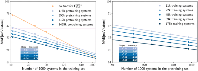
In the left panel of Fig. 3 we can see the MAE on the test set for predicting E^SCAN_hull, plotted on a log–log scale as a function of the number of systems in the training set. The different curves correspond to pre-training using PBE datasets of different size, while the orange curve shows the performance of the network trained without transfer learning.

We can observe that the points draw lines with very similar slopes for pre-training datasets of different sizes. In fact, the slope decreases only slightly with the increasing size of the pre-training dataset. This behavior is expected, as when more PBE data is already given to the model, less new information can be found in the additional SCAN data. The MAE decreases significantly and consistently with the increasing size of the pre-training set. The neural network trained only on the SCAN dataset (no transfer) has the largest MAE in all cases, even when the pre-training dataset is reduced by a factor of 10.

In the right panel of Fig. 3 we demonstrate that also the error as a function of the size of the pre-training dataset can be fitted by a line in the log–log graph. Here the slopes are smaller than in the left panel. Consequently, similar reductions of the MAE can be achieved by transfer learning at the cost of using significantly more pre-training data than training data. On the other hand, extra pre-training data can be generated with lower-level approximations at a reduced computational cost, and the pre-trained model can be used as a starting point for the training of several new models.

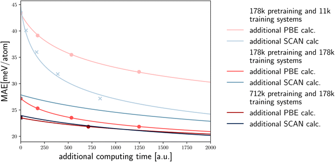
It is important to comment on the cost of calculations of the same property using different DFT functionals. For example, SCAN calculations are at least five time more expensive than PBE calculations. Calculations using hybrid functionals are even more computationally demanding. In the latter case, the possibility to use larger pre-training datasets to reduce the MAE of a predicted property becomes even more appealing and effective (Fig. 5).

Fig. 5 Based on the linear fits to the log–log plots, we demonstrate the expected MAE for the prediction of the SCAN distance to the convex hull when additional computing budget is allocated to either SCAN or PBE calculations. We present the predictions in relation to the computing time for various initial sizes of the training and pre-training sets, under the assumption that SCAN calculations are five times as expensive as PBE calculations.

To illustrate the potential of transfer learning based on the available high-fidelity (SCAN) and low-fidelity (PBE) data, and the relative computational cost of these calculations, we depict various scenarios in Fig. 5. For each case, we display the data points from our computational experiments as crosses/dots and extrapolate based on the previous fits. The first two lines represent scenarios with 178 k pre-training and 11 k training systems, showing a decrease in error based on additional PBE calculations and SCAN calculations versus the increased computational cost (assuming SCAN calculations are five times more expensive). In this case performing SCAN calculations is far more efficient in reducing the SCAN error.

However, when the number of pre-training and training systems is equal, additional PBE calculations become a more efficient approach (in terms of computer time) to improve the SCAN error. Ultimately, when there are four times as many pre-training systems, the computational cost balances out, and PBE and SCAN calculations provide approximately the same level of improvement. It is important to note that as we shift towards more expensive high-fidelity calculations, such as hybrid functionals, the balance further moves towards additional PBE calculations.

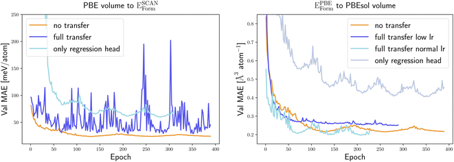
Seeing the promising results of transfer learning on two datasets of calculations of the same property, we also attempted to apply transfer learning to predict different properties. We consider therefore transfer learning to predict SCAN formation energies and PBEsol volumes, starting from neural networks trained to output PBE volumes and PBE formation energies, respectively.

As we can see in Fig. 6 only retraining the output network does not improve the performance of the model. This is true for both examples selected here and we can expect this to be a general rule. In fact, the strong dependence of the graph embeddings on the low-dimensional features that are good descriptors for a specific property makes this part of the network strongly property dependent.

Fig. 6 Learning curves, i.e., MAE on the validation set as a function of the training epoch, for the prediction of PBEsol volumes with transfer learning from a model pre-trained for E^PBE_form (left panel) and for the prediction of E^SCAN_form from a model pre-trained for PBE volumes (right panel). The different curves are obtained with the training procedures described in the text: without pre-training (no transfer), with pre-training using 1.8 M PBE calculations and freezing part of the weights (only regression head) and with pre-training using 1.8 M PBE calculations and successive full reoptimization of all weights (full transfer). In the right panel we consider full transfer with two different learning rates (lr).

We observe that reoptimizing all weights of the neural network, starting from the model pre-trained to predict another PBE property, leads to a very unstable learning curve and does not produce better results than training from scratch. To enforce convergence we retrained the full network with a learning rate 10 times smaller than before. This improves marginally the situation for transfer learning for the prediction of PBEsol volumes from PBE formation energies. However, the lower learning rate leads the neural network to settle down very quickly in a suboptimal local minimum from which it is unable to escape, yielding a model that is still worse than the one obtained from training on the PBEsol dataset only.

We have to conclude that two properties such as formation energy and optimized volume, are too far dissimilar to perform successful transfer learning. Of course, it is always possible that an extensive hyperparameter variation would improve this result. However, in this case, a hyperparameter search with the same resources should be performed also for the original model to make a valid comparison. Nevertheless, we attempted to use two more learning rates, lr = 1.25 × 10⁻⁵, 1.25 × 10⁻⁶ and additional weight decays of 0.01, 0.001 and 0.0001 but could not find any significant improvement.

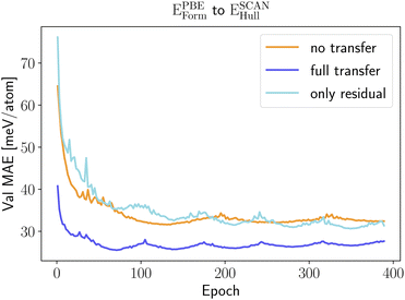
Transfer learning between a neural network that predicts PBE formation energies and a neural network that outputs SCAN energy distances to the convex hull performs better as these two properties are closely related. In Fig. 7 we can see that only retraining the regression head does not bring a significant error reduction. On the other hand, the full retraining is now able to improve considerably the model performance with an error reduction of 18%.

Fig. 7 Learning curves, i.e., MAE on the validation set as a function of the training epoch, for the prediction of E^SCAN_form with transfer learning from a neural network that predicts accurately E^PBE_hull. The different curves are obtained with the training procedures described in the text: without pre-training (no transfer), with pre-training using 1.8 M PBE calculations and freezing part of the weights (only regression head) and with pre-training using 1.8 M PBE calculations and successive full reoptimization of all weights (full transfer).

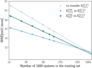
In Fig. 8 we compare the MAE on the validation set for the prediction of E^SCAN_form as a function of the training set size, considering the case of no transfer learning, and two approaches for transfer learning, either starting from a neural network pre-trained on the same property calculated with PBE or on E^PBE_hull. As expected, the intra-property transfer learning performs better, providing an 56–59% larger improvement than the inter-property transfer learning for the whole range of considered training set sizes.

Fig. 8 Log–log plot of the MAE on the validation set for the prediction of E^SCAN_form as a function of the training set size for a model trained solely on SCAN data (no transfer), a model pre-trained on a dataset of E^PBE_form calculations and a model pre-trained on E^PBE_hull calculations. The lines indicate a log–log linear fit to the data.

III. Conclusions

We demonstrated that performing transfer learning using a crystal graph neural network trained on a large (>10⁶) dataset of less accurate but faster calculations enables efficient training of the same neural network on a smaller (≈10⁴ − 10⁵) dataset of more accurate calculations. The final prediction error is significantly lower compared to the error that would be obtained if the neural network was trained from scratch only on the smaller dataset. We demonstrated that the obtained performance improvement is consistent when we perform transfer learning for different functionals and similar electronic properties, e.g., E_form, E_hull. Thanks to transfer learning, we can assume that a training set of about 10⁴ high-quality ab initio calculations is sufficient to obtain predictions of electronic quantities with chemical precision. High-throughput studies involving tens of thousands of calculations using advanced electronic structure methods are foreseeable in the near future. Transfer learning may therefore have a strong impact on future machine learning studies in solid-state physics, allowing prediction of properties with unprecedented accuracy.

We also demonstrated that the learning error after transfer learning decreases with increasing size of the pre-training dataset with a linear scaling in a log–log graph. Using this property, we can determine the relative size of the pre-training and training datasets, which allows us to minimize the prediction error and, at the same time, the total computational cost, given the different computational resources required for less accurate and more accurate ab initio calculations. This is of particular interest for training universal force fields, an emerging application of machine learning that has attracted increasing attention in recent years (see, e.g.,⁹). In fact, universal force fields are trained on PBE data so far. Since these force fields also use universal message-passing networks, we expect that transfer learning can also be easily applied to efficiently train the existing force fields to the quality of higher-fidelity functionals.

Unfortunately, our results show that transfer learning is only effective for physically similar electronic properties. If the pre-trained property is too dissimilar, the pre-training may actually paralyze the neural network in predicting the new property. It is in that case more convenient to produce a large database of lower-quality calculations of the desired final property than to perform inter-property transfer learning.

IV. Methods

A. Data

Our main PBE dataset consists of calculations from the Materials Project database,⁵⁵ AFLOW⁵⁶ and our own calculations. This set of around two million compounds was accumulated in ref. 18 and 35. In ref. 24 we reoptimized the geometries of 175 k materials using PBEsol followed by a final energy evaluation with the PBEsol and SCAN functional as described in ref. 24. By now we extended these datasets by another 50 k randomly selected materials arriving at 225 k entries.

In Fig. 9a we can see the element distribution of the PBE dataset. This set features a large variety of elements with oxygen and nitrogen being the most prominent followed by lithium. Not included are the noble gases and heavy radioactive chemical elements. In the elemental distribution of the PBEsol and SCAN dataset, depicted in Fig. 9b, oxygen is even more prevalent while nitrogen and hydrogen appear less often. This is a result of the many stable oxides in the PBE dataset.

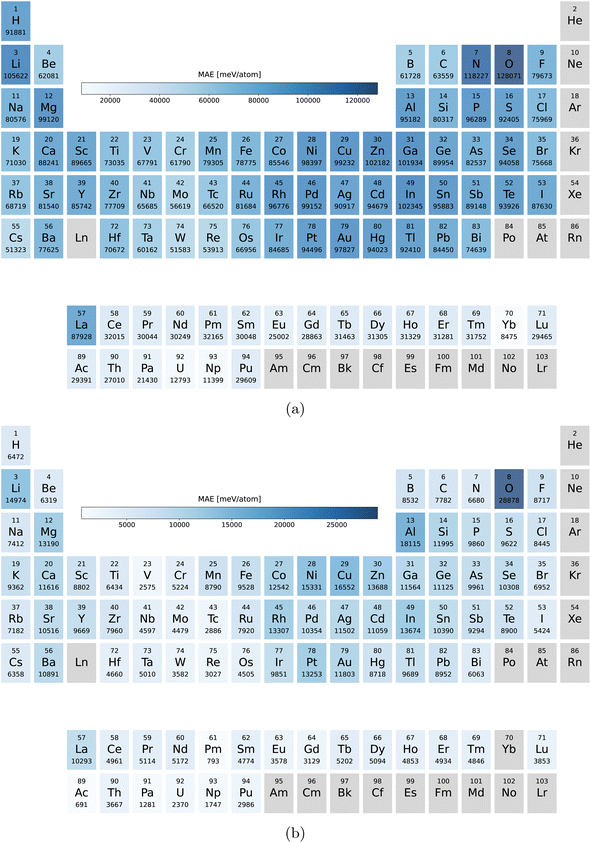Fig. 9 Number of the compounds containing each elements (a) in the PBE dataset and (b) in the PBEsol/SCAN dataset.

In Fig. 2 we plot the distribution of the various datasets we used in this work. As expected the materials of the PBEsol/SCAN dataset are on average far more stable with only a small long tail in the E_form and E_hull distributions introduced by the 50 k random systems. The differences in the distributions also show that the results are valid for transfer learning between datasets with rather different distributions. The volume dataset on the other hand is very similarly distributed for PBE and PBEsol with respective medians/means/standard deviations of 22.1/23.5/9.2 ų per atom and 18.7/19.9/7.4 ų per atom. The slightly higher median and mean of the PBE dataset are expected due to the underbinding of the PBE that is somewhat corrected by PBEsol. The distribution of the band gaps was already discussed earlier but the main difference is the percentage of metals that is roughly 4 times larger in the PBE dataset.

B. Crystal graph attention networks

Crystal graph attention networks were developed in ref. 35 for the discovery of new stable materials. Using the periodic graph representation of the crystal structure, the networks apply an attention based message passing mechanism. By using solely the graph distance of the atoms to their neighbors as edge information, CGATs can perform precise predictions based on unrelaxed geometries. If we compare the inputs for PBE and PBEsol geometries, there is generally a change in volume between the two, however, this does not necessarily result in a different input neighbor list (for example, for a cubic structure the input would stay the same). Only if the cell constants change relative to each other or the internal atomic positions change, the input to the network can also differ for the different functionals. We generally expect, however, that this results in a larger similarity of representations in comparison to standard force-field style networks using exact distances benefiting the transfer learning.

Following the notation of ref. 35, we label the embedding of the ith node, i.e., atom, at time steps t of the message passing process as hti and the respective edge embedding to the atoms j as etij. FCNNNt,na is the network of the nth attention head at message passing step t and HFCNNθgtt a hypernetwork depending on the difference between the embedding at step t and the previous step. Using this notation we arrive at the following equations for the updates of the node embeddings:

s^t,n_ij = FCNNN^t,n_a (h^t_i‖h^t_j‖e_ij) (1a)

m^t,n_ij = FCNN^t,n_m(h^t_i‖h^t_j‖e_ij). (1c)

The edges are updated similarly:

s^e,n_ij = FCNNNⁿ_a (h^t_i‖h^t_j‖e^t_ij) (2a)

m^e,n_ij = FCNNNⁿ (h^t_i‖h^t_j‖e^t_ij) (2c)

In parallel a ROOST³⁴ model calculates a representation vector of the composition that is used as a global context vector and is concatenated with the final node embeddings. Lastly, an attention layer calculates the embedding for the whole crystal structure. Then a residual network transforms the graph embedding into the prediction. We used the following hyperparameters: AdamW; learning rate: 0.000125; starting embedding: matscholar-embedding;⁵⁷ nbr-embedding-size: 512; msg-heads: 6; batch-size: 512; max-nbr: 24; epochs: 390; loss: L1-loss; momentum: 0.9; weight-decay: 1 × 10⁻⁶; atom-fea-len: 128; message passing steps: 5; roost message passing steps: 3; other roost parameters: default; vector-attention: true; edges: updated; learning rate: cyclical; learning rate schedule: (0.1, 0.05); learning rate period: 130 (70 for transfer learning, 90 for pre-training during the experiments shown in Fig. 3); hypernetwork: 3 hidden layers, size 128; hypernetwork activation function: tanh; FCNN: 1 hidden layer, size 512; FCNN activation function: leaky RELU;⁵⁸ Nvidia apex mixed precision level 02 (almost FP16) or 00.

Data availability

This study was carried out using publicly available data from https://doi.org/10.24435/materialscloud:5j-9m and https://doi.org/10.24435/materialscloud:m7-50. Additional SCAN and PBEsol data were added to https://doi.org/10.24435/materialscloud:5j-9m. The CGAT code is available at https://github.com/hyllios/CGAT and at https://zenodo.org/badge/latestdoi/352292655. The trained models resulting from all the experiments are available at https://tddft.org/bmg/data.php and at https://doi.org/10.5281/zenodo.8143755.

Author contributions

JS and NH performed the training of the machines and the machine learning predictions of the distance to the hull; MALM performed the DFT high-throughput calculations; JS, SB and MALM directed the research; all authors contributed to the analysis of the results and to the writing of the manuscript.

Conflicts of interest

The authors declare that they have no competing interests.

Acknowledgements

The authors gratefully acknowledge the Gauss Centre for Supercomputing e.V. (https://www.gauss-centre.eu) for funding this project by providing computing time on the GCS Supercomputer SUPERMUC-NG at Leibniz Supercomputing Centre (https://www.lrz.de) under the project pn25co. This project received funding from the European Union's HORIZON-MSCA-2021-DN-01 program under grant agreement number 101073486 (EUSpecLab).

References

1. A. C. Mater and M. L. Coote, Deep Learning in Chemistry, J. Chem. Inf. Model., 2019, 59(6), 2545–2559,  DOI:10.1021/acs.jcim.9b00266.
2. J. Vamathevan, D. Clark, P. Czodrowski, I. Dunham, E. Ferran and G. Lee, et al., Applications of machine learning in drug discovery and development, Nat. Rev. Drug Discovery, 2019, 18(6), 463–477.
3. J. Schmidt, M. R. G. Marques, S. Botti and M. A. L. Marques, Recent advances and applications of machine learning in solid-state materials science, npj Comput. Mater., 2019, 5(1), 83.
4. H. J. Kulik, T. Hammerschmidt, J. Schmidt, S. Botti, M. A. L. Marques and M. Boley, et al., Roadmap on Machine learning in electronic structure, Electron. Struct., 2022, 4(2), 023004,  DOI:10.1088/2516-1075/ac572f.
5. G. L. W. Hart, T. Mueller, C. Toher and S. Curtarolo, Machine learning for alloys, Nat. Rev. Mater., 2021, 6(8), 730–755,  DOI:10.1038/s41578-021-00340-w.
6. G. Pilania, Machine learning in materials science: from explainable predictions to autonomous design, Comput. Mater. Sci., 2021, 193, 110360 . Available from: https://www.sciencedirect.com/science/article/pii/S0927025621000859.
7. C. Chen, W. Ye, Y. Zuo, C. Zheng and S. P. Ong, Graph Networks as a Universal Machine Learning Framework for Molecules and Crystals, Chem. Mater., 2019, 31(9), 3564–3572.
8. T. Xie and J. C. Grossman, Crystal Graph Convolutional Neural Networks for an Accurate and Interpretable Prediction of Material Properties, Phys. Rev. Lett., 2018, 120(14), 145301.
9. X. Fu, Z. Wu, W. Wang, T. Xie, S. Keten and R. Gomez-Bombarelli, et al., Forces are not Enough: Benchmark and Critical Evaluation for Machine Learning Force Fields with Molecular Simulations, TMLR, 2023.
10. X. Fu, Z. Wu, W. Wang, T. Xie, S. Keten, R. Gomez-Bombarelli, et al., Forces are not Enough: Benchmark and Critical Evaluation for Machine Learning Force Fields with Molecular Simulations, arXiv, 2022, preprint, arXiv:221007237.
11. A. Dunn, Q. Wang, A. Ganose, D. Dopp and A. Jain, Benchmarking materials property prediction methods: the Matbench test set and Automatminer reference algorithm, npj Comput. Mater., 2020, 6(1), 138,  DOI:10.1038/s41524-020-00406-3.
12. J. S. Smith, R. Zubatyuk, B. Nebgen, N. Lubbers, K. Barros and A. E. Roitberg, et al., The ANI-1ccx and ANI-1x data sets, coupled-cluster and density functional theory properties for molecules, Sci. Data, 2020, 7(1), 1–10.
13. J. P. Perdew, K. Burke and M. Ernzerhof, Generalized Gradient Approximation Made Simple, Phys. Rev. Lett., 1996, 77, 3865–3868.
14. S. Curtarolo, W. Setyawan, G. L. W. Hart, M. Jahnatek, R. V. Chepulskii and R. H. Taylor, et al., AFLOW: an automatic framework for high-throughput materials discovery, Comput. Mater. Sci., 2012, 58, 218–226.
15. J. E. Saal, S. Kirklin, M. Aykol, B. Meredig and C. Wolverton, Materials Design and Discovery with High-Throughput Density Functional Theory: The Open Quantum Materials Database (OQMD), JOM, 2013, 65(11), 1501–1509.
16. S. Kirklin, J. E. Saal, B. Meredig, A. Thompson, J. W. Doak and M. Aykol, et al., The Open Quantum Materials Database (OQMD): assessing the accuracy of DFT formation energies, npj Comput. Mater., 2015, 1, 15010.
17. A. Jain, S. P. Ong, G. Hautier, W. Chen, W. D. Richards and S. Dacek, et al., Commentary: the Materials Project: a materials genome approach to accelerating materials innovation, APL Mater., 2013, 1(1), 011002.
18. J. Schmidt, N. Hoffmann, H. C. Wang, P. Borlido, P. J. Carriço, T. F. Cerqueira, et al., Large-Scale Machine-Learning-Assisted Exploration of the Whole Materials Space, arXiv, 2022, preprint, arXiv:221000579,  DOI:10.48550/arXiv.2210.00579.
19. T. Thonhauser, V. R. Cooper, S. Li, A. Puzder, P. Hyldgaard and D. C. Langreth, Van der Waals density functional: self-consistent potential and the nature of the van der Waals bond, Phys. Rev. B: Condens. Matter Mater. Phys., 2007, 76, 125112,  DOI:10.1103/PhysRevB.76.125112.
20. K. Jcv, D. R. Bowler and A. Michaelides, Van der Waals density functionals applied to solids, Phys. Rev. B: Condens. Matter Mater. Phys., 2011, 83, 195131,  DOI:10.1103/PhysRevB.83.195131.
21. K. Choudhary, K. F. Garrity, A. C. E. Reid, B. DeCost, A. J. Biacchi and A. R. H. Walker, et al., The joint automated repository for various integrated simulations (JARVIS) for data-driven materials design, npj Comput. Mater., 2020, 6, 173,  DOI:10.1038/s41524-020-00440-1.
22. K. Choudhary, Q. Zhang, A. C. E. Reid, S. Chowdhury, N. V. Nguyen and Z. Trautt, et al., Computational screening of high-performance optoelectronic materials using OptB88vdW and TB-mBJ formalisms, Sci. Data, 2018, 5(1), 180082.
23. K. Choudhary, G. Cheon, E. Reed and F. Tavazza, Elastic properties of bulk and low-dimensional materials using van der Waals density functional, Phys. Rev. B, 2018, 98, 014107.
24. J. Schmidt, H. C. Wang, T. F. T. Cerqueira, S. Botti and M. A. L. Marques, A new dataset of 175 k stable and metastable materials calculated with the PBEsol and SCAN functionals, Sci. Data, 2021, 12(1), 180082.
25. R. Kingsbury, A. S. Gupta, C. J. Bartel, J. M. Munro, S. Dwaraknath and M. Horton, et al., Performance comparison of r2SCAN and SCAN metaGGA density functionals for solid materials via an automated, high-throughput computational workflow, Phys. Rev. Mater., 2022, 6(1), 013801.
26. J. P. Perdew, A. Ruzsinszky, G. I. Csonka, O. A. Vydrov, G. E. Scuseria and L. A. Constantin, et al., Restoring the Density-Gradient Expansion for Exchange in Solids and Surfaces, Phys. Rev. Lett., 2008, 100, 136406,  DOI:10.1103/PhysRevLett.100.136406.
27. J. Sun, A. Ruzsinszky and J. P. Perdew, Strongly constrained and appropriately normed semilocal density functional, Phys. Rev. Lett., 2015, 115(3), 036402.
28. J. W. Furness, A. D. Kaplan, J. Ning, J. P. Perdew and J. Sun, Accurate and Numerically Efficient r2SCAN Meta-Generalized Gradient Approximation, J. Phys. Chem. Lett., 2020, 11(19), 8208–8215,  DOI:10.1021/acs.jpclett.0c02405.
29. J. Sun, R. C. Remsing, Y. Zhang, Z. Sun, A. Ruzsinszky and H. Peng, et al., Accurate first-principles structures and energies of diversely bonded systems from an efficient density functional, Nat. Chem., 2016, 8(9), 831–836.
30. R. Hussein, J. Schmidt, T. Barros, M. A. Marques and S. Botti, Machine-learning correction to density-functional crystal structure optimization, MRS Bull., 2022, 47(8), 765–771,  DOI:10.1557/s43577-022-00310-9.
31. P. Borlido, J. Schmidt, A. W. Huran, F. Tran, M. A. L. Marques and S. Botti, Exchange–correlation functionals for band gaps of solids: benchmark, reparametrization and machine learning, npj Comput. Mater., 2020, 6(1), 96.
32. Y. Zhang, D. A. Kitchaev, J. Yang, T. Chen, S. T. Dacek and R. A. Sarmiento-Pérez, et al., Efficient first-principles prediction of solid stability: towards chemical accuracy, npj Comput. Mater., 2018, 4(1), 9,  DOI:10.1038/s41524-018-0065-z.
33. C. W. Park and C. Wolverton, Developing an improved crystal graph convolutional neural network framework for accelerated materials discovery, Phys. Rev. Mater., 2020, 4, 063801.
34. R. E. A. Goodall and A. A. Lee, Predicting materials properties without crystal structure: deep representation learning from stoichiometry, Nat. Commun., 2020, 11(1), 6280,  DOI:10.1038/s41467-020-19964-7.
35. J. Schmidt, L. Pettersson, C. Verdozzi, S. Botti and M. A. L. Marques, Crystal graph attention networks for the prediction of stable materials, Sci. Adv., 2021, 7(49), eabi7948,  DOI:10.1126/sciadv.abi7948.
36. C. Tan, F. Sun, T. Kong, W. Zhang, C. Yang and C. Liu, A survey on deep transfer learning, in International Conference on Artificial Neural Networks, Springer, 2018, pp. 270–279.
37. K. S. Kalyan, A. Rajasekharan and S. Sangeetha, A Survey of Transformer-Based Pretrained Models in Natural Language Processing, J. Biomed. Inf. , 2022, 126, 103982.
38. M. L. Hutchinson, E. Antono, B. M. Gibbons, S. Paradiso, J. Ling and B. Meredig, Overcoming Data Scarcity with Transfer Learning, arXiv, 2017, preprint, arXiv:171105099,  DOI:10.48550/arXiv.1711.05099.
39. D. Jha, K. Choudhary, F. Tavazza, W. K. Liao, A. Choudhary and C. Campbell, et al., Enhancing materials property prediction by leveraging computational and experimental data using deep transfer learning, Nat. Commun., 2019, 10(1), 1–12.
40. J. S. Smith, B. T. Nebgen, R. Zubatyuk, N. Lubbers, C. Devereux and K. Barros, et al., Approaching coupled cluster accuracy with a general-purpose neural network potential through transfer learning, Nat. Commun., 2019, 10(1), 1–8.
41. S. Kong, D. Guevarra, C. P. Gomes and J. M. Gregoire, Materials representation and transfer learning for multi-property prediction, Appl. Phys. Rev., 2021, 8(2), 021409,  DOI:10.1063/5.0047066.
42. V. Gupta, K. Choudhary, F. Tavazza, C. Campbell, W. keng Liao and A. Choudhary, et al., Cross-property deep transfer learning framework for enhanced predictive analytics on small materials data, Nat. Commun., 2021, 12(1), 6595,  DOI:10.1038/s41467-021-26921-5.
43. H. Yamada, C. Liu, S. Wu, Y. Koyama, S. Ju and J. Shiomi, et al., Predicting Materials Properties with Little Data Using Shotgun Transfer Learning, ACS Cent. Sci., 2019, 5(10), 1717–1730,  DOI:10.1021/acscentsci.9b00804.
44. E. Ford, K. Maneparambil, A. Kumar, G. Sant and N. Neithalath, Transfer (machine) learning approaches coupled with target data augmentation to predict the mechanical properties of concrete, Mach. Learn. Appl., 2022, 8, 100271,  DOI:10.1016/j.mlwa.2022.100271.
45. A. Kolluru, N. Shoghi, M. Shuaibi, S. Goyal, A. Das and C. L. Zitnick, et al., Transfer learning using attentions across atomic systems with graph neural networks (TAAG), J. Chem. Phys., 2022, 156(18), 184702,  DOI:10.1063/5.0088019.
46. C. Chen, Y. Zuo, W. Ye, X. Li and S. P. Ong, Learning properties of ordered and disordered materials from multi-fidelity data, Nat. Comput. Sci., 2021, 1(1), 46–53.
47. S. Feng, H. Zhou and H. Dong, Application of deep transfer learning to predicting crystal structures of inorganic substances, Comput. Mater. Sci., 2021, 195, 110476 . Available from: https://www.sciencedirect.com/science/article/pii/S0927025621002019.
48. P. P. De Breuck, G. Hautier and G. M. Rignanese, Materials property prediction for limited datasets enabled by feature selection and joint learning with MODNet, npj Comput. Mater., 2021, 7(1), 1–8.
49. C. Chen and S. P. Ong, AtomSets as a hierarchical transfer learning framework for small and large materials datasets, npj Comput. Mater., 2021, 7(1), 1–9.
50. L. Chanussot, A. Das, S. Goyal, T. Lavril, M. Shuaibi and M. Riviere, et al., Open Catalyst 2020 (OC20) Dataset and Community Challenges, ACS Catal., 2021, 11(10), 6059–6072,  DOI:10.1021/acscatal.0c04525.
51. S. Chmiela, A. Tkatchenko, H. E. Sauceda, I. Poltavsky, K. T. Schütt and K. R. Müller, Machine learning of accurate energy-conserving molecular force fields, Sci. Adv., 2017, 3(5), e1603015,  DOI:10.1126/sciadv.1603015.
52. J. Schmidt, L. Chen, S. Botti and M. A. L. Marques, Predicting the stability of ternary intermetallics with density functional theory and machine learning, J. Chem. Phys., 2018, 148(24), 241728.
53. J. Schmidt, J. Shi, P. Borlido, L. Chen, S. Botti and M. A. L. Marques, Predicting the Thermodynamic Stability of Solids Combining Density Functional Theory and Machine Learning, Chem. Mater., 2017, 29(12), 5090–5103,  DOI:10.1021/acs.chemmater.7b00156.
54. J. Schmidt, H. Wang, G. Schmidt and M. Marques, Machine Learning Guided High-throughput Search of Non-Oxide Garnets, npj Comput. Mater., 2023, 9, 63,  DOI:10.1038/s41524-023-01009-4.
55. A. Jain, S. P. Ong, G. Hautier, W. Chen, W. D. Richards and S. Dacek, et al., Commentary: the Materials Project: a materials genome approach to accelerating materials innovation, APL Mater., 2013, 1(1), 011002,  DOI:10.1063/1.4812323.
56. S. Curtarolo, W. Setyawan, G. L. Hart, M. Jahnatek, R. V. Chepulskii and R. H. Taylor, et al., AFLOW: an automatic framework for high-throughput materials discovery, Comput. Mater. Sci., 2012, 58, 218–226,  DOI:10.1016/j.commatsci.2012.02.005.
57. V. Tshitoyan, J. Dagdelen, L. Weston, A. Dunn, Z. Rong and O. Kononova, et al., Unsupervised word embeddings capture latent knowledge from materials science literature, Nature, 2019, 571(7763), 95–98.
58. S. S. Liew, M. Khalil-Hani and R. Bakhteri, Bounded activation functions for enhanced training stability of deep neural networks on visual pattern recognition problems, Neurocomputing, 2016, 216, 718–734.

---