 Open Access Article
Go with the flow: deep learning methods for autonomous viscosity estimations†
Michael
Walker
,
Gabriella
Pizzuto
 ,
Hatem
Fakhruldeen
and
Andrew I.
Cooper
 *
*
Department of Chemistry, University of Liverpool, L69 3BX, UK. E-mail: aicooper@liverpool.ac.uk
First published on 4th September 2023
Abstract
Closed-loop experiments can accelerate material discovery by automating both experimental manipulations and decisions that have traditionally been made by researchers. Fast and non-invasive measurements are particularly attractive for closed-loop strategies. Viscosity is a physical property for fluids that is important in many applications. It is fundamental in application areas such as coatings; also, even if viscosity is not the key property of interest, it can impact our ability to do closed-loop experimentation. For example, unexpected increases in viscosity can cause liquid-handling robots to fail. Traditional viscosity measurements are manual, invasive, and slow. Here we use convolutional neural networks (CNNs) as an alternative to traditional viscometry by non-invasively extracting the spatiotemporal features of fluid motion under flow. To do this, we built a workflow using a dual-armed collaborative robot that collects video data of fluid motion autonomously. This dataset was then used to train a 3-dimensional convolutional neural network (3D-CNN) for viscosity estimation, either by classification or by regression. We also used these models to identify unknown laboratory solvents, again based on differences in fluid motion. The 3D-CNN model performance was compared with the performance of a panel of human participants for the same classification tasks. Our models strongly outperformed human classification in both cases. For example, even with training on fewer than 50 videos for each liquid, the 3D-CNN model gave an average accuracy of 88% for predicting the identity of five different laboratory solvents, compared to an average accuracy of 32% for human observation. For comparison, random category selection would give an average accuracy of 20%. Our method offers an alternative to traditional viscosity measurements for autonomous chemistry workflows that might be used both for process control (e.g., choosing not to pipette liquids that are too viscous) or for materials discovery (e.g., identifying new polymerization catalysts on the basis of viscosification).
Introduction
Autonomous robots and self-driving laboratories can significantly accelerate experiments by performing repetitive tasks that are traditionally carried out by hand.1–3 These laboratory tasks are often time consuming, leaving less time for researchers to spend on cognitive activity. There are several advantages to automating laboratory experiments such as increased throughput, improved safety, stronger data protocols and auditability and, in some cases, improved repeatability. A fundamental requirement for autonomous laboratory robots is the ability to measure different physical properties using fast and, where possible, non-invasive techniques that can be integrated into end-to-end workflows. Such automated measurements allow the autonomous closed-loop optimization of physical properties for materials such as photocatalytic activity,4 solubility,5 and thin-film performance.6Viscosity is a measure of a fluid's resistance to flow caused by internal friction of fluid layers during motion. It is a fundamental property that is important in a wide range of applications such as lubricants, oil recovery,7 3D printing technologies, inks and coatings,8 and in chemical formulations for sectors such as pharmaceuticals,9 agrochemicals, food,10 and home and personal care. Viscosity is also an important parameter in material discovery labs; for example, the viscosity of a liquid can provide information about the current state in a chemical synthesis workflow.3,11 Perhaps less obviously, viscosity is a basic consideration in material handling using robots since all liquid handlers have some upper limit, and usually a lower limit, for the viscosity of the fluids that they can handle. This can cause problems when a liquid handling robot attempts to handle a fluid that has become more viscous or gelled during a chemical reaction, for example during a polymerization.
Viscosity is a difficult property to measure in an automated way. Fluids can be divided into two classes: Newtonian fluids, where the viscosity is independent of shear rate, and non-Newtonian fluids, where the viscosity depends on the shear rate. Non-Newtonian fluids can exhibit shear thickening or thinning, where the viscosity either increases or decreases with shear rate,12 making them particularly challenging to characterize. Even for Newtonian fluids, however, it is non-trivial to incorporate viscosity measurements into automated workflows. There are various kinds of viscometers. Falling sphere viscometers drop a sphere inside a tube of fluid and track its motion, correlating the terminal velocity of the sphere with viscosity. Rotational viscometers measure the torque required to keep a rotating spindle or disk immersed in a fluid at a constant speed. Capillary viscometers relate viscosity to the time taken for a fluid to discharge through a capillary tube and can operate on a microlitre scale, achieving accuracies of 2 percent with as little as 20 μL of fluid.13 However, microfluidic viscometers typically require extensive cleaning14 and can suffer from chip degradation or obstruction of the channels.15 Likewise, high-throughput rotational viscometer platforms exist,16 but they are usually expensive, and samples often need to be reformatted to be presented to the instrument. As well as introducing an additional reformatting step, this raises a fundamental problem for fully automated discovery workflows: that is, certain samples may simply become too viscous to be reformatted by a liquid handling robot, and the entire workflow could fail on that basis. As such, there is value in developing noninvasive viscosity estimation methods for automated workflows.
Various invasive techniques have already been developed to estimate rheological properties using robotic platforms. Lopez-Guevara et al.17 proposed a method for learning rheological properties of fluids by attaching a stirrer to a robot and manipulating the fluid. The physical properties of the fluid were learned by synchronising simulated and real stirring actions until the simulation converged towards the real-world setup. Such models were then applied to pouring tasks and the amount of spillage was the evaluation metric. Hence, this approach used a robot to learn the rheological properties through manipulations and then transferred that to a robotic pouring task. For a materials discovery workflow, however, this strategy is less appealing because it requires the manipulation (stirring) of each sample, which in turn necessitates operations such as decapping and re-capping of vials. Soh et al.14 developed an automated pipetting robot to measure viscosity of Newtonian fluids with viscosities between 1500–12![[thin space (1/6-em)]](https://www.rsc.org/images/entities/char_2009.gif) 000 cP. Here, the liquid handling robot aspirates a fluid and dispenses it into well plate under fixed dispensing conditions. The viscosity was estimated from the flow rate or weight of fluid dispensed. This method could measure viscosity with an error of 6.5% and it is a simple and relatively inexpensive alternative to traditional viscometers, making it appealing for autonomous materials research. A similar approach was adopted by Deshmukh et al.18 However, these approaches are again invasive and would add additional manipulations into an automated workflow. It is also likely that accuracy will decrease at higher viscosities, and the method could fail entirely in cases where the robot attempts to pipette a sample that has in fact gelled.
000 cP. Here, the liquid handling robot aspirates a fluid and dispenses it into well plate under fixed dispensing conditions. The viscosity was estimated from the flow rate or weight of fluid dispensed. This method could measure viscosity with an error of 6.5% and it is a simple and relatively inexpensive alternative to traditional viscometers, making it appealing for autonomous materials research. A similar approach was adopted by Deshmukh et al.18 However, these approaches are again invasive and would add additional manipulations into an automated workflow. It is also likely that accuracy will decrease at higher viscosities, and the method could fail entirely in cases where the robot attempts to pipette a sample that has in fact gelled.
In addition to invasive measurements, there are also methods to model and therefore predict viscosity. For example, the viscosity of glycerol can be modelled using a four-parameter correlation considering both temperature and concentration,19 but this is material specific. Arrhenius and William–Landel–Fessey (WLF) models have been used to estimate the viscosity of liquid foods,20 with the latter being applied to heavy oils.21 There are also models to estimate viscosity of gases.22 However, these methods are not generalisable and they obviously cannot be applied to materials discovery workflows that involve diverse arrays of materials where the full compositional and structural details of the samples are unknown.
Non-invasive viscosity measurements that do not require physical models are particularly attractive for automated or autonomous workflows. Computer vision and machine learning are powerful tools for measuring properties such as solubility5,23 and for material identification.24,25 These approaches exploit autonomous systems that visually inspect samples, typically with a camera, and then make a decision; a simple skill for humans but still an open challenge for laboratory robots. In principle, the viscosity of fluids can be estimated by analysing the visual features of the fluid undergoing motion. Hence, machine vision-based methods have the potential to provide a faster, non-invasive estimate of fluid viscosity.
Convolutional neural networks (CNNs) are deep learning models specifically designed for image processing, utilising convolutional layers to automatically extract meaningful features from the input images, allowing for highly accurate pattern recognition and classification tasks. Since fluids with different viscosities behave differently in motion, CNNs have the potential to model viscosity from video data. Previously, J. van Assen et al.26 trained a slow fusion model to estimate the viscosities of sixteen different liquids ranging from 1–10![[thin space (1/6-em)]](https://www.rsc.org/images/entities/char_2009.gif) 000 cP. In that study, the flow of the liquids was simulated, rather than measured, across a range of scenarios such as pouring, stirring, and raining. The CNN model's performance was compared with human observations. Hyperparameters were optimised to match human performance and representational similarity analysis was used to compare known image metrics (e.g., colour and edge detection) to the model performance. While this work gives insight into how humans perceive viscosity, it uses fluid simulations, as opposed to real data, which again cannot be used in automated materials discovery scenarios, as discussed above.25 In related work, Mohan and Menon27 used pretrained models to estimate the viscosity of fluids, again from simulated data, by combining a CNN model with a recurrent neural network (RNN).
000 cP. In that study, the flow of the liquids was simulated, rather than measured, across a range of scenarios such as pouring, stirring, and raining. The CNN model's performance was compared with human observations. Hyperparameters were optimised to match human performance and representational similarity analysis was used to compare known image metrics (e.g., colour and edge detection) to the model performance. While this work gives insight into how humans perceive viscosity, it uses fluid simulations, as opposed to real data, which again cannot be used in automated materials discovery scenarios, as discussed above.25 In related work, Mohan and Menon27 used pretrained models to estimate the viscosity of fluids, again from simulated data, by combining a CNN model with a recurrent neural network (RNN).
In an experimental study, Jafari and Tatar28 used data of fluid flow to estimate the behaviour of date syrup. Images of syrup moving freely through orifices were captured and the extracted numerical features from these images were fed into a neural network to estimate fluid flow behavior. This approach uses real data but it involves additional apparatus to acquire the images; effectively, the need to flow through an orifice makes the method invasive from an automation standpoint.
Here we developed an alternative method where a dual-arm robot collects data autonomously by manipulating fluid samples while capturing visual data. The fluid motion, captured through videos, was then used to train deep learning models for viscosity estimation and lab liquid identification. The method is fast (one video takes approximately 1 minute to collect), non-invasive, and can be used for samples where the composition is unknown, and hence where the use of models is impossible.
Specifically, our method uses 3 dimensional-convolutional neural networks (3D-CNNs) to estimate the viscosities of different fluids. We also explored the use of these models to identify unknown fluids by classification. The latter task was motivated by the fact that many laboratory samples are colourless and visually similar, even under close inspection. We also compared the performance of our deep learning model with the ability of human participants to predict viscosity ranges and to identify liquid samples. Our autonomous robotic system outperformed human skill significantly for both tasks.
Methods
Sample preparation and dataset
Samples of aqueous honey were prepared by mixing water and honey to provide a range of viscosities between 350–13![[thin space (1/6-em)]](https://www.rsc.org/images/entities/char_2009.gif) 150 cP. Honey was chosen because it exhibits Newtonian behaviour.29,30 Air bubbles and the formation of crystals can affect the viscosity of honey;31 to reduce the presence of both, we followed the sample preparation procedure reported by Yanniotis et al.31 The viscosity of each test sample was recorded using a conventional viscometer (Brookfield DV-II + Pro). A range of general-purpose Newtonian viscosity standards were also used, purchased from Paragon Scientific. The aqueous honey and viscosity standard samples were prepared in 40 mL laboratory vials in 20 mL quantities. We also investigated the classification (i.e., identification) of 5 common laboratory solvents: acetone, dimethyl sulfoxide (DMSO), isopropanol, ethanol and water. For these experiments, we prepared 2 mL samples in 8 mL vials.
150 cP. Honey was chosen because it exhibits Newtonian behaviour.29,30 Air bubbles and the formation of crystals can affect the viscosity of honey;31 to reduce the presence of both, we followed the sample preparation procedure reported by Yanniotis et al.31 The viscosity of each test sample was recorded using a conventional viscometer (Brookfield DV-II + Pro). A range of general-purpose Newtonian viscosity standards were also used, purchased from Paragon Scientific. The aqueous honey and viscosity standard samples were prepared in 40 mL laboratory vials in 20 mL quantities. We also investigated the classification (i.e., identification) of 5 common laboratory solvents: acetone, dimethyl sulfoxide (DMSO), isopropanol, ethanol and water. For these experiments, we prepared 2 mL samples in 8 mL vials.
Full details of the test materials used and the video dataset are shown in Table 1. The videos of the five common solvents (collectively LabLiquids) were 4 seconds long and were recorded at 15 frames per second (FPS). The videos of the viscosity standards were 15 seconds long and were recorded at 30 FPS. The videos of the aqueous honey samples were 6 seconds long and were recorded at 15 FPS. All videos had a resolution of 1024 × 576 pixels. The videos were recorded in a working Chemistry lab, and no specific controlled lighting was used.
| Liquid | No. of videos | Amount (mL) | Vial size (mL) | Viscosity range (cP) |
|---|---|---|---|---|
| Viscosity standards | 163 | 20 | 40 | 2150–26![[thin space (1/6-em)]](https://www.rsc.org/images/entities/char_2009.gif) 400 400 |
| Aqueous honey | 164 | 20 | 40 | 350–13![[thin space (1/6-em)]](https://www.rsc.org/images/entities/char_2009.gif) 150 150 |
| Acetone | 48 | 2 | 10 | 0.36 |
| Water | 47 | 2 | 10 | 0.9 |
| DMSO | 47 | 2 | 10 | 2.0 |
| Isopropanol | 41 | 2 | 10 | 2.4 |
| Ethanol | 40 | 2 | 10 | 1.2 |
Model overview
For all experiments, we used a 3D-CNN to extract the spatiotemporal features from the frames from the video dataset. The 3D-CNN structure comprises two 3-dimensional convolutional layers, each with a 3-dimensional batch normalisation, rectified linear unit (ReLU) activation function and max pooling. Three fully connected layers were used to map the features to the final output of the network. We set the output of the final fully connected layer to 1 for regression, and the number of classes, which in our case was 5, for classification. A random seed was set to 0 for all models to ensure reproducibility. Dropout was also set to 0,32 and we used an Adam optimiser.33 Early stopping was used to prevent overfitting.34 For regression, gradient clipping with a threshold of 10 was used to prevent gradient explosion.35 Each model required a selection of frames from the dataset. For viscosity estimation, we kept the frame distribution even between the first and last sections of the video. For identification of liquid contents, we used a non-linear distribution. We optimised the batch size and learning rates and stored the values that lead to the best models.For the classification approach, we computed the cross-entropy loss and accuracy on the test set. Cross entropy (CE) loss measures the difference between two probability distributions: the target distribution (the actual viscosity category) and the predicted one (the model's predictions of the viscosity category). Accuracy was derived from the model's predictions by considering the class associated with the maximum activation for a given input.
For the regression models, the mean squared error (MSE) loss was used. The MSE is the average of the squared differences between the actual and predicted viscosity. The root mean square error (RMSE), mean absolute error (MAE) and R2 values were used to evaluate model performance on the test data.
The framework is powered by PyTorch,‡ using a machine equipped with an Intel(R) Core(TM) i9-10980XE CPU @ 3.00 GHz 36 Core CPU.
Autonomous robot system
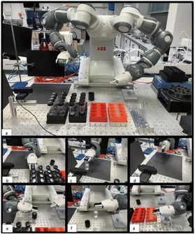
The robotic setup comprised the YuMi collaborative robot, which is a dual-arm, seven degree-of-freedom platform. The use of two arms facilitated the movement of vials from station to station. The setup is shown in Fig. 1. Briefly, a Logitech webcam§ and racks containing the capped sample vials were placed within the workspace of the robot. The camera was not mounted on the robotic platform since the total payload per arm of this particular robot is less than 0.5 kg, which would limit the objects (vials) that the robot could manipulate.In this workflow, the robot picked up the sample to be tested from a rack, manipulated it in front of the camera (by rotation) to capture the video stream, and then transferred it to another rack for storage. An overview of this sequence of operations is shown in Fig. 1. The videos captured the vial being rotated up to 90° while recording the associated fluid motion. A video of the data collection workflow can be found here https://youtu.be/C_YJFU8h5vs. The videos were recorded in a working Chemistry lab, and no specific lighting was used. In the case shown in the video, the robot estimated the viscosity of the samples and sorted them into one of three groups; (i) ‘good’ samples, where the viscosity is within a desired specification range (green storage rack); (ii) ‘bad’ samples where the viscosity is outside of this specification range (red storage rack), and; (iii) ‘borderline’ samples, earmarked for re-testing, where the model cannot reliably classify the viscosity because the difference between the estimated viscosity and the specification range limits is comparable to the error in the CNN model.
A full video of the procedure can be found here https://youtu.be/C_YJFU8h5vs. While the sample storage capacity in the workflow is 16 (two storage racks with 8 samples), this is effectively unlimited in a closed-loop workflow since we can use a mobile robot to deliver samples to the analysis rack and remove them from the storage racks for longer-term storage elsewhere.
Human participant comparison study
To compare the performance of the CNN models with human performance for viscosity estimation and liquid classification tasks, we assembled a human panel to carry out the same tasks (10 panel participants; 4 female, 6 male). All panellists were undergraduate chemistry students and were hence familiar with solvents and laboratory settings. The experiment was approved through the Ethics Committee at the University of Liverpool. This panel experiment was split into two parts. First, participants were asked to predict the viscosity class for a subset of the videos from the ViscoVids dataset. In the second test, participants were asked to identify unknown samples of the 5 solvents discussed above by visual evaluation in closed vials.For initial training to estimate viscosity, each participant was shown two videos from the five different viscosity classes to familiarise them with the fluid motion for these viscosity ranges. The five viscosity classes were labelled very low (1000–5000 cP), low (5001–9000 cP), medium (9001–13![[thin space (1/6-em)]](https://www.rsc.org/images/entities/char_2009.gif) 000 cP), high (1
000 cP), high (1![[thin space (1/6-em)]](https://www.rsc.org/images/entities/char_2009.gif) 300
300![[thin space (1/6-em)]](https://www.rsc.org/images/entities/char_2009.gif) 117
117![[thin space (1/6-em)]](https://www.rsc.org/images/entities/char_2009.gif) 000 cP) and very high (over 17
000 cP) and very high (over 17![[thin space (1/6-em)]](https://www.rsc.org/images/entities/char_2009.gif) 000 cP) by the human supervisor. The participants were then shown 10 unlabelled, randomised videos (2 from each viscosity category) and asked to label each in terms of its viscosity. Participants were informed that there were two videos belonging to each category. The overall experiment took 10 minutes to complete. Each video was randomly selected from each category. All videos were shown from start to finish, each lasting 20 seconds. There was roughly a 10 second gap between participants guessing the class of one video before moving onto the next. There was no time limit to answer, but on average, each participant predicted the class for each video in roughly 5 seconds. Participants were also allowed to change their previous answers based on later videos in the experiment. Each experiment lasted for about 30 minutes.
000 cP) by the human supervisor. The participants were then shown 10 unlabelled, randomised videos (2 from each viscosity category) and asked to label each in terms of its viscosity. Participants were informed that there were two videos belonging to each category. The overall experiment took 10 minutes to complete. Each video was randomly selected from each category. All videos were shown from start to finish, each lasting 20 seconds. There was roughly a 10 second gap between participants guessing the class of one video before moving onto the next. There was no time limit to answer, but on average, each participant predicted the class for each video in roughly 5 seconds. Participants were also allowed to change their previous answers based on later videos in the experiment. Each experiment lasted for about 30 minutes.
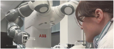
For estimation of solvent identities, each participant was seated in front of the robotic platform (Fig. 2) and asked to observe the autonomous rotated vial and then label it as acetone, water, DMSO, ethanol or isopropanol. For training, each participant was shown 3 examples of each solvent used in the test. There was a 10 second gap before the next sample was shown to allow time for participants to familiarise themselves with each liquid's movement. After this, participants were given 20 unknown samples (4 trials for each solvent) and were asked to label the contents. The participants were informed that there was 4 samples of each liquid. The rotation speed was 25 mm s−1, which is the same speed the samples were rotated for the LabLiquids dataset. The vials were also the same size (8 mL), containing the same amount of liquid (2 mL) as the LabLiquids dataset. Each sample was rotated for 5 seconds prior to prompting the participant for an estimated label. The samples were presented to the participant via the robotic platform every 15 seconds.
The average time for each experiment was about 40 minutes; no time limit was strictly given to a participant for each estimation, but each answer took around 5 seconds. As before, participants were allowed to change their previous answers based on later samples in the experiment.
Our autonomous robotic workflow was evaluated for two main tasks: (1) estimation of fluid viscosity across a range of different fluids and viscosities by using either classification or regression, and; (2) identification of fluids, based on differences in fluid motion under dynamic conditions, by classification.
Autonomous viscosity estimation
First, the performance of the CNN model was evaluated for its ability to estimate the viscosity of fluids covering a wide range of viscosities using commercial viscosity standards and aqueous honey samples. For this experiment, we evaluated the model performance both by using classification and by using regression.The normalised confusion matrix for viscosity standard estimation into viscosity ranges is shown in Fig. 3. Five viscosity categories were defined: very low (1000–5000 cP), low (50![[thin space (1/6-em)]](https://www.rsc.org/images/entities/char_2009.gif) 009
009![[thin space (1/6-em)]](https://www.rsc.org/images/entities/char_2009.gif) 000 cP), medium (9000–13
000 cP), medium (9000–13![[thin space (1/6-em)]](https://www.rsc.org/images/entities/char_2009.gif) 000 cP), high (13
000 cP), high (13![[thin space (1/6-em)]](https://www.rsc.org/images/entities/char_2009.gif) 000–17
000–17![[thin space (1/6-em)]](https://www.rsc.org/images/entities/char_2009.gif) 000 cP) and very high (greater than 17
000 cP) and very high (greater than 17![[thin space (1/6-em)]](https://www.rsc.org/images/entities/char_2009.gif) 000 cP). The model accuracy was found to be 87.5%.
000 cP). The model accuracy was found to be 87.5%.
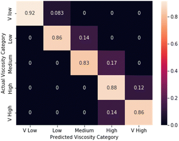 | ||
| Fig. 3 Confusion matrix for viscosity estimation using a 3D-CNN model for the commercial viscosity standards dataset (average performance = 87.5%). | ||
Results and discussion
In this set of 40 test samples, there were five samples that were misclassified by the model. Fig. 4 labels these five samples and shows their true viscosities; each of the five misclassified samples was found to be close to a category boundary, further validating the model performance.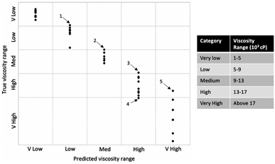 | ||
| Fig. 4 Modified confusion matrix to display the actual viscosity values of the five videos (labelled 1–5 on the graph) that were misclassified by the 3D-CNN model. | ||
For the regression models, the Mean Squared Error (MSE) loss was used. The MSE is the average of the squared differences between the actual and predicted viscosity. The root mean square error (RMSE), mean absolute error (MAE) and R2 values were used to evaluate model performance on the test data, as illustrated in Table 2. The regression model showed good performance at estimating the commercial viscosity standards dataset, especially considering the large range of viscosity used in the experiment. The model estimating aqueous honey samples performed somewhat less well when the errors were compared to the viscosity spread.
| Liquid | RMSE (cP) | MAE (cP) | R 2 |
|---|---|---|---|
| Viscosity standard | 1400 | 1039 | 0.94 |
| Aqueous honey | 497 | 414 | 0.96 |
Autonomous solvent identity classification
In this experiment, we evaluated the CNN model for the task of predicting the identity of 5 typical chemistry solvents using video information alone. The same experimental procedure was used as for viscosity estimation of commercial viscosity standards. The model showed an excellent performance, with an accuracy of 88% (Fig. 5). This is surprising given the similarity of these five liquids, which are all colourless and have low viscosity.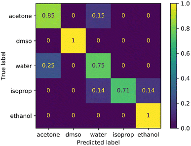 | ||
| Fig. 5 Confusion matrix for autonomous classification of solvent identity using a 3D-CNN model (average performance = 88%). | ||
Comparison of model classification with human classification
We next compared the performance of the CNN models with human performance for viscosity estimation and liquid classification tasks. The human panel experiment was split into two parts. First, participants were asked to predict the viscosity class (very_low ≤ viscosity ≤ very_high) for a subset of the videos from the ViscoVids dataset. In the second test, participants were asked to identify unknown samples of the 5 solvents discussed above by visual evaluation in closed vials. For the viscosity estimation task, the CNN model outperformed human observation significantly, with an accuracy score of 87.5% compared to an average human participant score of 53%. The confusion matrix for the human panel's estimation of viscosity is shown in Fig. 6. Participants correctly predicted the very low and very high viscosities most frequently, but struggled to distinguish viscosity ranges between these two extremes, thus showing the superiority of the CNN model for finer detail classifications. Moreover, some panellists confused the very high and very low viscosity classes, a mistake that was never made by the CNN model (Fig. 3). There was no significant asymmetry about the diagonal in the confusion matrix for the panel's viscosity estimation (Fig. 6); that is, there was no evidence for a systematic underestimation or overestimation of viscosity.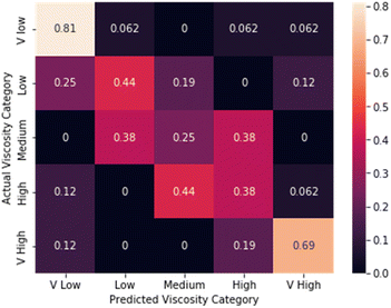 | ||
| Fig. 6 Confusion matrix for estimation of solvent viscosity by a panel of 10 human participants for the commercial viscosity standards dataset (average performance = 53%). | ||
For the solvent classification task, we compared machine vision classification with human classification in a similar way. The performance of the human participants is illustrated in Fig. 7. This is a challenging task for humans because the visual differences between most of these solvents are subtle. Again, the CNN model outperformed human observation for this task significantly: the model performance was 88% compared to an average performance of 32% for human participants.
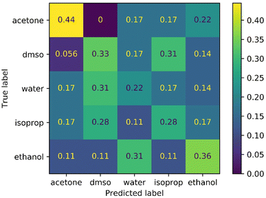 | ||
| Fig. 7 Confusion matrix for classification of solvent identity by a panel of 10 human participants (average performance = 32%). | ||
Participants correctly identified acetone more frequently than any other liquid, which is the least viscous of the solvents and hence behaves more distinctively under flow. By contrast, the panel's identification of water, in particular, was only a little better than chance. We note that panellists were also aware that there were four samples of each liquid and were allowed to change their answers. This gave a small additional positive bias for the human participants to deduce the solvent identity because the CNN had no such information.
Discussion
We used relatively small datasets in these proof of concept experiments. Typically, video classification tasks are trained on thousands of images per class, containing multiple variations of the object or class, while here the largest datasets used were relatively small: 163 videos for the commercial viscosity standards and 164 videos for the aqueous honey samples. For the five solvents, fewer than 50 videos of each solvent were used to train the model. While the ability to surpass human classification with a small training set offers some practical advantages, we would also expect that a larger training library might improve the model robustness and quality. Future work will focus on increasing the dataset size, using different sized vials, and altering the video background. An advantage of this robotic method is the significant reduction in time required to collect these datasets autonomously, particularly when coupled in the future with the use of mobile robots to load and unload the workcell,4 which will allow continuous throughput.The differences between the number of frames used for model input, hyper optimisation values, and number of iterations for each model result from the computational time. This led to a trade-off between computational resources and model performance. For example, the model for the viscosity standards regression experiment achieved good performance with only 10 frames per video, and we could therefore afford to use more resources on the batch size and a greater number of iterations for training. It is worth mentioning that the overarching goal of this study was to keep the method accessible to a wide range of laboratories,36 while retaining very good model performance on low computational resources.
It is challenging to unpack the precise manner by which the CNN classifies viscosity, but for the identification of the five solvents, we explored the model performance with a varied distribution of selected frames as an input. Manual inspection of the video frames suggested more easily noticeable differences in the liquid appearance, at least to the human eye, at the start and the end of the video. This observation aligned with experiments, since a non-linear distribution of frames for the model's input gave the highest accuracy.
Previous studies have sought to understand the way that humans perceive fluid viscosity,26,37–39 but all used simulated liquid scenarios with no background variation (e.g., in terms of lighting variation), as is present in a real laboratory. Here we worked with experimental data rather than simulated data, which makes this method applicable to unknown fluid compositions in a materials discovery scenario where the viscosity cannot, by definition, be simulated.
While the accuracy of our method for viscosity estimation is clearly lower than for a standard industrial viscometer (e.g., Brookfield viscometers are within 1% error of the full scale range), our approach is much faster (approximately one video acquired per minute), more compatible with automation workflows, and inexpensive. Since the method is non-invasive, there is also no need to uncap or re-cap the sample vials. This suggests a number of potential use cases. A robust five-level viscosity classification scheme (Fig. 3 and 4) could be used to reject samples that are beyond a certain tolerance – for example, to avoid wasting time and resources with more accurate but expensive measurements for material compositions that are clearly out of the target specification. The potential for this is illustrated by a video of the workflow that demonstrates autonomous sample sorting (https://youtu.be/C_YJFU8h5vs). Likewise, most liquid handling robots cannot manipulate samples with high viscosities, or samples that have gelled, and this classification approach might be used to prevent such attempts, which have the potential to cause an entire workflow to fail. Beyond workflow control tasks, this non-invasive approach could be used for discovering new chemistry; for example, in rapidly screening for new polymerization catalysts by identifying combinations that lead to a significant viscosity change. The method could also be adapted to the discovery of materials such as hydrogels40 or organogels, and to better understand their gelation kinetics. With more training and refinement, this method might also be used to extract polymerization kinetics in automated workflows without the need for invasive sampling methods such as gel permeation chromatography.
Data availability
ESI† including code and data have been uploaded to https://github.com/cooper-group-uol-robotics/go-with-the-flow. A detailed demonstration video can be found at: https://youtu.be/C_YJFU8h5vs.Conflicts of interest
There are no conflicts to declare.Acknowledgements
We acknowledge funding from Engineering and Physical Sciences Research Council (EPSRC case award no. 17100099), the Leverhulme Trust via the Leverhulme Research Centre for Functional Materials Design and the ERC ADAM Synergy grant (grant agreement no. 856405). We thank Unilever for financial support and Ellen Piercy for support as an industrial liaison during this project. A. I. C. thanks the Royal Society for a Research Professorship (RSRP\S2\232003).References
- B. P. MacLeod, F. G. L. Parlane, A. K. Brown, J. E. Hein and C. P. Berlinguette, Nat. Mater., 2022, 21, 722–726 CrossRef CAS PubMed
.
- M. Christensen, L. P. Yunker, F. Adedeji, F. Häse, L. M. Roch, T. Gensch, G. dos Passos Gomes, T. Zepel, M. S. Sigman and A. Aspuru-Guzik,
et al.
, Commun. Chem., 2021, 4, 112 CrossRef PubMed
.
- C. D. Abernethy, G. M. Codd, M. D. Spicer and M. K. Taylor, J. Am. Chem. Soc., 2003, 125, 1128–1129 CrossRef CAS PubMed
.
- B. Burger, P. M. Maffettone, V. V. Gusev, C. M. Aitchison, Y. Bai, X. Wang, X. Li, B. M. Alston, B. Li, R. Clowes, N. Rankin, B. Harris, R. S. Sprick and A. I. Cooper, Nature, 2020, 583, 237–241 CrossRef CAS PubMed
.
-
G. Pizzuto, J. de Berardinis, L. Longley, H. Fakhruldeen and A. I. Cooper, 2022 International Joint Conference on Neural Networks, IJCNN, 2022, pp. 1–7 Search PubMed
.
- B. P. MacLeod, F. G. L. Parlane, T. D. Morrissey, F. Häse, L. M. Roch, K. E. Dettelbach, R. Moreira, L. P. E. Yunker, M. B. Rooney, J. R. Deeth, V. Lai, G. J. Ng, H. Situ, R. H. Zhang, M. S. Elliott, T. H. Haley, D. J. Dvorak, A. Aspuru-Guzik, J. E. Hein and C. P. Berlinguette, Sci. Adv., 2020, 6, 8867 CrossRef PubMed
.
- R. G. Santos, W. Loh, A. C. Bannwart and O. V. Trevisan, Braz. J. Chem. Eng., 2014, 571–590 CrossRef
.
- J. Lisowski, B. Szadkowski and A. Marzec, Materials, 2022, 15, 4961 CrossRef CAS PubMed
.
- J. Elliott, J. L. McConaha, N. Cornish, E. Bunk, L. Hilton, A. Modany and I. Bucker, J. Pharm. Technol., 2014, 30, 111–117 CrossRef CAS PubMed
.
- C. Miyazawa, K. Sakagami, N. Konno and Y. Nonomura, Technologies, 2020, 8, 1–9 CrossRef
.
- W. Jung, C. Hurth, A. Becker and F. Zenhausern, Sens. Bio-Sens. Res., 2015, 12, 8–12 CrossRef
.
-
T. Mezger, The Rheology Handbook, Vincentz Network, Hannover, Germany, 2020 Search PubMed
.
- L. H. Phu Pham, L. Bautista, D. C. Vargas and X. Luo, RSC Adv., 2018, 8, 30441–30447 RSC
.
- B. W. Soh, A. Chitre, W. Y. Lee, D. Bash, J. N. Kumar and K. Hippalgaonkar, Digital Discovery, 2023, 2, 481–488 RSC
.
- V. Carnicer, C. Alcázar, M. Orts, E. Sánchez and R. Moreno, Open Ceram., 2021, 5, 100052 CrossRef CAS
.
- J. Läuger and M. Krenn, AIP Conf. Proc., 2008, 1198–1201 CrossRef
.
-
T. Lopez-Guevara, R. Pucci, N. K. Taylor, M. U. Gutmann, S. Ramamoorthy and K. Suhr, 2020 IEEE/RSJ International Conference on Intelligent Robots and Systems, IROS, 2020, pp. 5351–5357 Search PubMed
.
- S. Deshmukh, M. T. Bishop, D. Dermody, L. Dietsche, T.-C. Kuo, M. Mushrush, K. Harris, J. Zieman, P. Morabito, B. Orvosh and D. Patrick, ACS Comb. Sci., 2016, 18, 405–414 CrossRef CAS PubMed
.
- N.-S. Cheng, Ind. Eng. Chem. Res., 2008, 47, 3285–3288 CrossRef CAS
.
- M. Peleg, Crit. Rev. Food Sci. Nutr., 2017, 58, 2663–2672 CrossRef PubMed
.
- S. Ilyin, M. Arinina, M. Polyakova, V. Kulichikhin and A. Malkin, Fuel, 2016, 186, 157–167 CrossRef CAS
.
- B. Najafi, Y. Ghayeb and G. A. Parsafar, Int. J. Thermophys., 2000, 21, 1011–1031 CrossRef CAS
.
- P. Shiri, V. Lai, T. Zepel, D. Griffin, J. Reifman, S. Clark, S. Grunert, L. P. Yunker, S. Steiner, H. Situ, F. Yang, P. L. Prieto and J. E. Hein, iScience, 2021, 24, 102176 CrossRef CAS PubMed
.
- S. Eppel, H. Xu, M. Bismuth and A. Aspuru-Guzik, ACS Cent. Sci., 2020, 6, 1743–1752 CrossRef CAS PubMed
.
- S. Eppel, H. Xu, Y. R. Wang and A. Aspuru-Guzik, Digital Discovery, 2022, 1, 45–60 RSC
.
- J. van Assen, S. Nishida and R. Fleming, PLoS Comput. Biol., 2020, 16, 1–29 CrossRef PubMed
.
-
V. Mohan M S and V. Menon, The First International Conference on AI-ML-Systems, New York, NY, USA, 2021 Search PubMed
.
- A. A. Jafari and E. Tatar, J. Agric. Mach., 2018, 8, 309–320 Search PubMed
.
- C. Faustino and L. Pinheiro, Foods, 2021, 10, 1–40 CrossRef PubMed
.
- P. Trávníček, T. Vítěz and A. Přidal,
et al.
, Sci. Agric. Bohemoslov., 2012, 43, 160–165 Search PubMed
.
- S. Yanniotis, S. Skaltsi and S. Karaburnioti, J. Food Eng., 2006, 72, 372–377 CrossRef
.
- N. Srivastava, G. Hinton, A. Krizhevsky, I. Sutskever and R. Salakhutdinov, J. Mach. Learn. Res., 2014, 15, 1929–1958 Search PubMed
.
-
D. P. Kingma and J. Ba, Proceedings of the 3rd International Conference on Learning Representations, ICLR, 2015, pp. 1–15 Search PubMed
.
- X. Ying, J. Phys.: Conf. Ser., 2019, 1–6 Search PubMed
.
-
R. Pascanu, T. Mikolov and Y. Bengio, Proceedings of the 30th International Conference on International Conference on Machine Learning, 2013, vol. 28, pp. 1310–1318 Search PubMed
.
- N. Rupp, K. Peschke, M. Köppl, D. Drissner and T. Zuchner, SLAS Technol., 2022, 27, 312–318 CrossRef PubMed
.
- T. Kawabe, K. Maruya, R. W. Fleming and S. Nishida, Vision Res., 2015, 109, 125–138 CrossRef PubMed
.
- V. C. Paulun, T. Kawabe, S. Nishida and R. W. Fleming, Vision Res., 2015, 115, 163–174 CrossRef PubMed
.
- J. van Assen, P. Barla and R. Fleming, Curr. Biol., 2018, 28, 452–458 CrossRef CAS PubMed
.
- E. R. Draper and D. J. Adams, Langmuir, 2019, 35, 6506–6521 CrossRef CAS PubMed
.
Footnotes |
| † Electronic supplementary information (ESI) available. See DOI: https://doi.org/10.1039/d3dd00109a |
| ‡ PyTorch v1.1.0 was used. |
| § Logitech C920 and C930 camera models were used. |
| This journal is © The Royal Society of Chemistry 2023 |

