An interpretable and transferrable vision transformer model for rapid materials spectra classification

Abstract

Rapid analysis of materials characterization spectra is pivotal for preventing the accumulation of unwieldy datasets, thus accelerating subsequent decision-making. However, current methods heavily rely on experience and domain knowledge, which not only proves tedious but also makes it hard to keep up with the pace of data acquisition. In this context, we introduce a transferable Vision Transformer (ViT) model for the identification of materials from their spectra, including XRD and FTIR. First, an optimal ViT model was trained to predict metal organic frameworks (MOFs) from their XRD spectra. It attains prediction accuracies of 70%, 93%, and 94.9% for Top-1, Top-3, and Top-5, respectively, and a shorter training time of 269 seconds (∼30% faster) in comparison to a convolutional neural network model. The dimension reduction and attention weight map underline its adeptness at capturing relevant features in the XRD spectra for determining the prediction outcome. Moreover, the model can be transferred to a new one for prediction of organic molecules from their FTIR spectra, attaining remarkable Top-1, Top-3, and Top-5 prediction accuracies of 84%, 94.1%, and 96.7%, respectively. The introduced ViT-based model would set a new avenue for handling diverse types of spectroscopic data, thus expediting the materials characterization processes.

---

Introduction

Global challenges in clean energy, sustainability, medicine and healthcare have sparked an unprecedented demand for innovative functional materials.¹ Given the urgency of these challenges, there is a compelling need to transition the research paradigm from a labor-intensive and empirical one to an autonomous one. This transformation spans several crucial stages, encompassing synthesis, characterization, performance testing, and informed decision making.^2–5 Within these stages, collection of characterization data assumes a paramount role. Spectroscopic techniques including X-ray diffraction (XRD), Fourier-transform infrared (FTIR), Raman, nuclear magnetic resonance (NMR), and mass spectrometry (MS), as well as microscopic methods like scanning electron microscopy, transmission electron microscopy, and atomic force microscopy, witness an exponential surge in acquisition. This necessitates real-time processing of this characterization data to prevent accumulation of the massive datasets, which otherwise could significantly impede the momentum of subsequent decision-making steps. But current mainstream data analysis practices predominantly rely on experience and domain knowledge, a process that is not only monotonous but also is incapable of matching the data acquisition pace. Consequently, it is highly desirable to establish a rapid and precise technique for processing characterization data with automation to expedite the advancement of novel materials.

Recent advances in machine learning (ML), especially deep learning (DL), offer an exciting opportunity to reshape scientific research within the domains of chemical and materials science.^6–8 This is particularly evident in facilitating rapid analysis of intricate data, including but not limited to XRD,^9,10 IR/FTIR,^11,12 Raman,^13,14 and MS data.^15,16 For example, Oviedo and coworkers have demonstrated deployment of convolutional neural networks (CNNs) to effectively classify the dimensionalities and space groups of thin-film metal halides from XRD spectra.⁹ This application showcases the potential of utilizing advanced DL techniques to enhance the accuracy and efficiency of materials characterization. Fine et al. developed CNNs for identifying functional groups of unknown compounds from fused FTIR and MS spectra.¹¹ Despite much progress, application of DL in spectrum analysis still faces several challenges. First, with the increase in input data size, CNNs may not be ideal for chemical spectra analysis because their filters have a local receptive field, limiting their ability to capture global patterns in the data.¹⁷ Furthermore, in the past studies, the DL models lack generality to be transferred across different materials and/or spectrum types. Consequently, one would need to initiate the training process for a new model from scratch for each distinct application.

Transformer, initially introduced in 2017 for sequential data processing,¹⁸ has become a predominant architecture for natural language processing (NLP). This is attributed to its adeptness in extracting broadly applicable representations from the textual information that it encodes. The self-attention layers inherent in the Transformer enable simultaneous handling of sequential data, overcoming challenges associated with long-range dependencies. This in turn facilitates efficient training of neural networks using extensive datasets. Built upon the foundation of the Transformer architecture, large language models like ChatGPT, Bard, LLaMA, and CLAUDE^19–22 have shown surprisingly emergent ability in generating text and performing zero- and few-shot learning scenarios. They hold significant promise across different application domains.²³ For instance, Transformer has paved the way to image recognition. This diversification into visual modalities is prominently illustrated by Vision Transformer (ViT).

With its success in processing sequential data, Transformer has recently demonstrated its versatility and far-reaching impact in chemical and materials sciences, spanning from literature mining to physiochemical property prediction.^24–28 An exemplary promise is reflected in its power for data analysis.^17,29–36 In a recent study, a Mass2SMILES model based on Transformer was employed to predict functional groups and SMILES descriptors from the high-resolution MS/MS spectra,²⁹ showing mean square errors (MSEs) of 0.0001 and 0.24 for the functional groups and SMILES descriptors, respectively. Another Transformer model was trained to predict molecular structures from the ¹H/¹³C NMR spectra, showing a Top-1 accuracy of 67%.³⁰ When the input ¹H NMR spectra are combined with a set of likely compounds, the Top-1 accuracy is increased to a remarkable value of 96%. In contrast to the MS and NMR spectra showing sharp, discrete peaks corresponding to the molecular features, XRD, Raman, and FTIR spectra often produce broader absorption or emission bands, reflecting a range of various features. These much-broadened bands would make it difficult for many ML/DL models to predict accurate results but could be well suited for the ViT models to handle. Very recently, a ViT model was developed to identify bacterial Gram types, species, and antibiotic-resistant strains in bloodstream infections from the surface-enhanced Raman scattering (SERS) spectra, achieving accuracies of 99.30% for classifying the Gram types and 97.56% for the species.³⁴ Despite the progress, application of ViT in characterization data analysis is still in its infancy. Particularly, exploration of their genericity for applications from one material to another and from one spectrum type to another has been quite limited if not any.

Herein, we demonstrate a transferable ViT model for accurate and rapid identification of metal organic frameworks (MOFs) and organic molecules from XRD and FTIR spectra, respectively. ViT for XRD (ViT-XRD) achieved prediction higher accuracies of 70%, 93%, and 94.9% for Top-1, Top-3, and Top-5, respectively, and a shorter training time of 269 seconds (∼30% faster) than those of CNN-XRD (60.4%, 88.1%, 89.9%, and 378 seconds, respectively). Fine hyperparameter tuning reveals that the length of the segmented spectra plays a critical role in determining the predicted outcomes. Dimension reduction by t-SNE shows that the ViT-XRD model is more adept at classifying these XRD spectra than the CNN-XRD model. The derived attention weight heatmap reveals that the ViT-XRD model exhibits concentrated attention on the minor peaks to distinguish very close spectra showing close characteristics of the primary peaks, while the CNN model more relies on the primary peaks to do so. Furthermore, the ViT-XRD model can be transferred for FTIR spectra classification of a different material type (organic molecules). This model is denoted as ViT-TL-FTIR. Classification of the FTIR spectra is a more difficult task since the characteristics of the FTIR spectra are much more irregular than those of the XRD spectra. Nevertheless, the ViT-TL-FTIR model achieved prediction accuracies of 84%, 94.1%, and 96.7% for Top-1, Top-3, and Top-5, respectively, which are much higher than those of the non-transferred one and the transferred one from the CNN model (CNN-TL-FTIR). It is worth noting that these results were attained without the noise reduction in the raw spectra, thereby drastically expediting the data analysis.

The contribution of this work can be summarized as follows. First, we innovated the use of a Vision Transformer architecture for classifying XRD spectra of MOFs, demonstrating higher prediction accuracies compared to those of the CNN models. Second, results from the dimension reduction and the attention weight map uncover the mechanism of discerning key features of the XRD spectra, thus improving the interpretability of the model. Third, transferability of a pre-trained model to a new one for analyzing the FTIR spectra of a different material type accentuates the generality of Transformer for this purpose, thus opening a new avenue to future research in integrating and synthesizing the diverse spectroscopic data sources, e.g., Raman, NMR, and MS. This integration can further be enriched by combining other chemical information, such as structures and properties of the materials, thereby developing a comprehensive and multifaceted approach to materials discovery.

Results and discussion

Development of CNN and ViT models

The architectures of CNN-XRD and ViT-XRD models are illustrated in Fig. 1. Derived from the LeNet-5 architecture, the CNN-XRD model is composed of multiple layers, each contributing to the overall model's functionality (Fig. 1a). This architecture includes an input layer, four convolutional blocks, one flattened layer, three fully connected layers, and an output layer. The input layer processes the complete XRD spectra spanning 2theta (2θ) in a range of 5–50°. Subsequently, the data undergoes a series of transformations with four consecutive convolution blocks. Each block comprises a convolutional layer responsible for feature extraction, a max pooling layer for spatial down-sampling, and a dropout layer to prevent overfitting. Following these convolutional operations, the data pass through a flattened layer followed by three fully connected layers. These layers enable the model to comprehend patterns within the data. Finally, the output layer affords the classification of the input data based on the operations in the preceding layers. The detailed architecture of the CNN-XRD model can be found in Fig. S1.†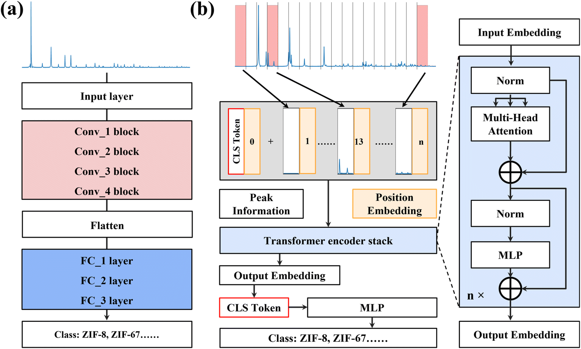

Fig. 1 Pipelines of (a) CNN-XRD and (b) ViT-XRD models.

The ViT-XRD model is constructed as a deep neural network, leveraging a self-attention mechanism as its foundation (Fig. 1b). It begins with segmenting the XRD spectra as the input. For the spectra that cannot be evenly segmented into an integer, the trailing portion of the data is discarded. Specifically, embedding of the spectra adds a class [CLS] token to symbolize the start of embedding. To capture positional information, position encoding is added to each segmented spectrum. Then, the embedding is processed by a sequence of the Transformer encoder stacks, each of which comprises a multi-head attention (MHA) layer and a multilayer perceptron (MLP) layer (right panel of Fig. 1b) with both residual connection and layer normalization. In each attention head, the input embedding is multiplied by three learnable weight vectors W_q, W_k, and W_v, transforming it into a query, key, and value vector (Q, K, and V). The scaled dot-product attention A is calculated from the equation: A = softmax((Q × K^T)/(d_k)^1/2) × V, where d_k denotes the dimension of Q and K. The randomly initialized W_q, W_k, and W_v vectors enable the ViT-XRD model to grasp contextual information in the segmented spectra. All attention heads are concatenated and then passed through the MLP for projecting the output to match the dimension of the embedded input. The self-attention mechanism permits the incorporation of information from the full spectra into individual embeddings. Consequently, each of these embeddings stands as a representative of the entire sequence. The encoder iterates this process through a defined number of layers, where a stochastic depth dropout is incorporated at each layer for additional regularization. Ultimately, only the [CLS] token enter an MLP regression layer for the output classification.

Datasets and data preprocessing

A total of 2000 theoretical MOF XRD spectra were sourced from the Cambridge Crystallographic Data Centre (CCDC) website and subsequently truncated to fit within a 2θ range spanning from 5 to 50°. Then, they were augmented by a factor of 200 using a physics-informed, three-step approach of peak elimination, scaling, and shift (Fig. S2†).⁹ Details can be referred to ESI Note S1.† Inspired by the augmentation techniques such as random crop and erasing in the domain of image classification,³⁷ instead of augmenting data in a fixed 2θ range,⁹ we augmented it in a randomized 2θ range to obtain more diverse training data. As a result, the trained model affords higher prediction accuracies, as depicted in Fig. S3.† To test the models, 30 experimental XRD spectra were collected from ten well-known MOFs that were synthesized by three different methods.¹⁰ These experimental XRD spectra were subjected to subsequent preprocessing steps of Savitzky–Golay smoothing and background subtraction (ESI Note S2†).⁹ Fig. S4† shows augmented, theoretical, and experimental XRD spectra of the ten representative MOFs. The augmented theoretical XRD spectra are split into training and validation datasets with a ratio of 4 : 1, while the experimental XRD spectra serve as the testing data.

Performance of ViT-XRD and CNN-XRD models

Fig. 2 depicts the performance of both CNN-XRD and ViT-XRD models. Each model was trained 100 times with slightly varied prediction accuracies and training durations each time. Their statistical results are reported here. The optimal ViT-XRD model shows average prediction accuracies for Top-1 (69.1%), Top-3 (93.2%), and Top-5 (94.9%), respectively, which are higher than those of the CNN-XRD model (60%, 87.6%, and 89.5%, respectively). This indicates that the ViT-XRD model can extract more critical features from the XRD spectra than the CNN-XRD model can. It is noteworthy that the ViT-XRD model requires an average training duration of 269 seconds, which is 110 seconds (∼30%) shorter than that of the CNN-XRD model. In comparison to the CNN-XRD model, the superior performance of the ViT-XRD model can be attributed to key factors such as the self-attention mechanism and parallelism.¹⁸ The self-attention mechanism in the Transformer architecture allows for efficient capture of long-range dependencies within the spectra, thereby facilitating faster convergence. Unlike CNNs that rely on local sliding windows to process sequences, Transformer is inherently designed for high parallelism. This enables them to perform computations simultaneously at different positions in a sequence, thus significantly reducing the training time.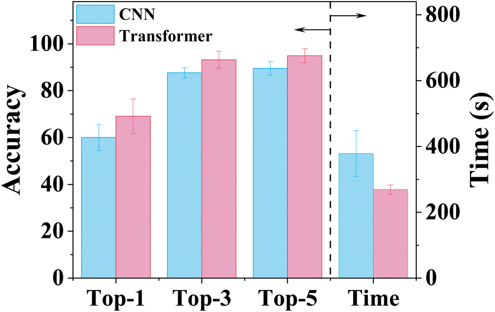

Fig. 2 Comparison performance of the CNN-XRD and ViT-XRD models in terms of prediction accuracies and training time.

In addition to the CNN-XRD and ViT-XRD models, five traditional ML models including Naïve Bayes (NB), k-nearest neighbors (KNNs), logistic regression (LR), random forest (RF), extreme gradient boosting (XGB) were also trained to classify the XRD spectra. As summarized in Table S1,† though impressive performance in performing various tasks,^7,38 the ensemble models including RF and XGB were found to be entirely inappropriate for spectra identification, requiring exorbitant computational times and yielding near-zero accuracies. NB exhibited prediction accuracies of less than 20% across Top-1 to Top-5 and training time of ∼4 seconds, while KNN showed higher prediction accuracies (36.7%, 63.3%, and 66.7%) and shorter training time (1.8 seconds). In contrast, LR, previously used for materials spectra analysis,^39,40 demonstrated pretty high prediction accuracies. However, it required a training time of 4100 seconds, which is >10 times longer than those of the CNN-XRD and ViT-XRD models. This is mainly because LR does not inherently support parallel computation and cannot fully utilize the advantage of parallelization capabilities embedded in modern GPUs.

Hyperparameter tuning for the ViT-XRD model

To improve model's generalizability and robustness, tuning the hyperparameters of the ViT-XRD model was performed using a grid search technique. Fig. 3 shows the prediction accuracies when three hyperparameters of Embed_dim, Depth, and Num_head are tuned. The Embed_dim sets the length of the segmented XRD spectra, directly influencing their positional information. As shown in Fig. 3a, the prediction accuracies increase with the increased Embed_dim, peaking at 66.9%, 94.6%, and 96.2% for Top-1, Top-3, and Top-5, respectively, when Embed_dim is 120. But a further increase in Embed_dim decreases the accuracies. Notably, the corresponding training time shows the opposite trend. Embed_dim of 120 requires the lowest training time of ∼420 s. Depth signifies the number of the Transformer's encoder stacks in deciphering intricate relationships within the spectra. As depicted in Fig. 3b, an optimal value of 7 for Depth achieves satisfactory prediction accuracies although a training time of 336 s is slightly larger than that achieved in the model trained with Depth of 4. Num_head governs the number of self-attention heads for parallel processing. The prediction accuracies for Top-1, Top-3, and Top-5 occur when Num_head is 4 without significantly increasing the training time (Fig. 3c). Hence, the optimal three hyperparameters were determined to be 120 for Embed_dim, 7 for Depths, and 4 for Num_head. To investigate the importance of these hyperparameters on performance, a set of decision trees was trained (ESI Note S3 and Fig. S5–S7†). The results from Fig. S5–S7† are summarized in Fig. 3d, revealing that Embed_dim plays the most important role in classifying the XRD spectra as it occupies an importance score of ∼90%, consistent with the analysis shown in Fig. 3a. When the number is larger or less than 120, the prediction accuracies are greatly reduced. Num_head takes ∼10% in the importance score, while the importance of Depth is negligible. It is worth noting that we tried many reasonable hyperparameter combinations. The afforded prediction accuracies by the ViT-XRD model are consistently higher than those by the CNN-XRD model.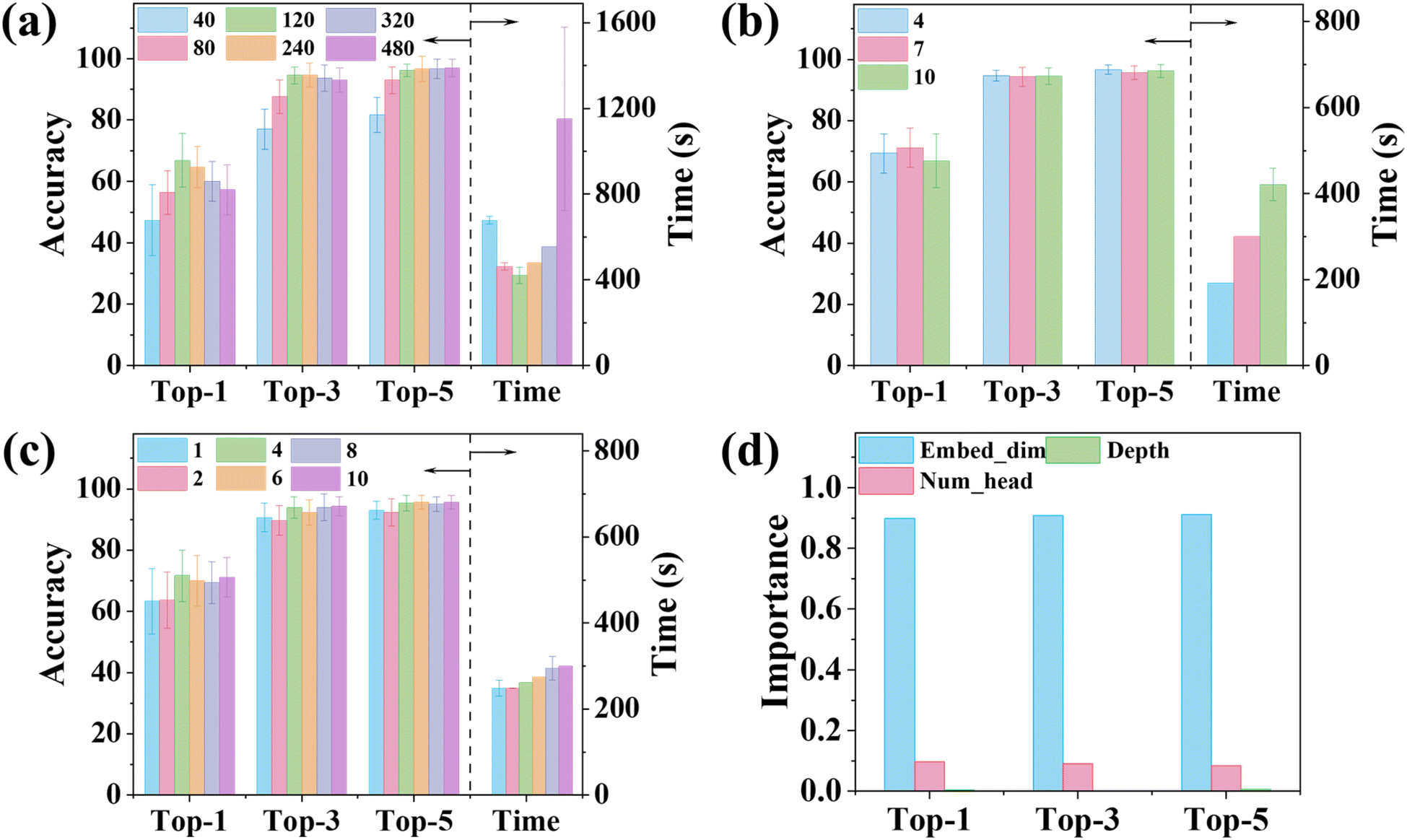

Fig. 3 Performance of the ViT-XRD models in terms of prediction accuracies and training time when trained with varied hyperparameters of (a) Embed_dim while setting Depth and Num_head to be 10 and 10, respectively; (b) Depth while setting Embed_dim and Num_head to be 120 and 10, respectively; and (c) Num_head while setting Embed_dim and Depth to be 120 and 7, respectively; (d) hyperparameter importance scores among Embed_dim, Depth, and Num_head.

Visualization of attention weight maps output from the ViT-XRD model

Understanding how the ViT model can efficiently classify the XRD spectra is quite desired. To do that, t-distributed stochastic neighbor embedding (t-SNE) was first employed. t-SNE is a dimensionality reduction technique commonly used in data visualization and pattern recognition.⁴¹ It represents the high-dimensional data in a lower-dimensional space while preserving the pairwise similarities among them. The t-SNE plot can reveal clusters, patterns, or structures that might appear in the original high-dimensional space. The t-SNE plot of the 2000 theoretical XRD spectra is depicted in Fig. 4a. It is evident that the XRD spectra sharing similar patterns are clustered together while those less similar spectra are furthered away, e.g., the dots representing MOF-2, MOF-5, ZIF-71, and ZIF-90 are scattered apart. Close observation shows that the dots belonging to ZIF-8 and ZIF-67 are overlapped, like those of ZIF-7 and ZIF-9, MOF-74 and MOF-199, which is consistent with the results shown in Fig. S3,† indicating similarity of their XRD spectra. The close similarity leads to the decreased prediction accuracy by the CNN-XRD model. But the ViT-XRD model seems to easily distinguish them. It inspires us to explore the mechanism behind it.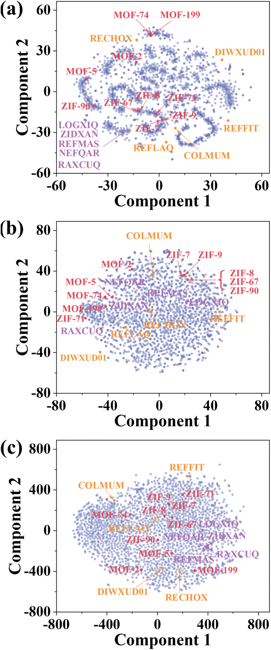

Fig. 4 t-SNE plots of (a) theoretical XRD spectra of 2000 MOFs, representations learned from (b) the CNN-XRD model and (c) the ViT-XRD model. Red: ten representative XRD spectra of MOFs. Purple: five MOFs with maximal distance to their respective nearest neighbors. Yellow: five most clustered MOFs. The CCDC numbers and full names of these 10 MOFs are listed in Table S2.†

To do that, representations of the corresponding spectra learned by the CNN-XRD and ViT-XRD models were visualized by t-SNE (Fig. 4b and c). Surprisingly, ZIF-8 and ZIF-67, MOF-74 and MOF-199, and ZIF-7 and ZIF-9 no longer overlapped. Instead, they are scattered and easily dispersible. But the representations extracted from the CNN-XRD model for ZIF-8, ZIF-67, and ZIF-90 still overlapped. This suggests that the ViT-XRD model is more adept at classifying these XRD spectra with higher accuracies than the CNN-XRD model. To test this hypothesis, two sets of spectra for a total of 10 MOFs were chosen. Details of selection criteria are explained in ESI Note S4,† and their full names are listed in Table S2.† The first set contains the five MOFs that are maximally distant from their nearest neighbors (yellow dots in Fig. 4a), which still maintain a distinguishable distance from other MOFs in t-SNE maps (yellow dots in Fig. 4b and c). The second set comprises another five MOFs that are the most closely clustered together (purple dots in Fig. 4a), which are widely distributed across the feature space by the CNN-XRD model with reduced localized concentration (purple dots in Fig. 4b). But the ViT-XRD model succeeds in dispersing them while still maintaining them within the same region, thereby retaining a visible indication of their intrinsic similarities (purple dots in Fig. 4c).

To deeply understand how these two models identify XRD spectra, two representative ZIFs including ZIF-8 and ZIF-67 sharing nearly similar XRD spectra were chosen. Fig. 5a presents the XRD spectra of ZIF-8 and ZIF-67, annotated with crystal planes at respective peaks. Obviously, three primary peaks at 7.4° and 12.8°, corresponding to the (011) and (012) planes are virtually identical for two ZIFs. In contrast, a few minor peaks located at 16.5°, 18.1°, 24.6°, and 26.8°, corresponding to the (013), (222), (233), and (134) planes, exhibit different intensities, which are the main disparities between these two spectra. Since CNN can't classify them while ViT can, herein, we aim to disclose how they make such different decisions. Heatmap, a graphical representation to visualize the intensity or importance of certain values/regions, is useful for interpreting the outcome of neural networks. For CNNs, a class activation map (CAM), highlighting the regions in the input spectra that most influence the classification result, was used for a comparative analysis.⁴² The CAMs for ZIF-8 and ZIF-67 were plotted by utilizing the output of the last convolutional layer of the CNN-XRD model, and the details can be found in the Methods. As shown in Fig. 5b and c, the red regions in CAMs reveal that the CNN-XRD model predominantly focuses on the two primary peaks at 7.4°, 12.8° with a slight blue-shift (∼3°) when making the classifying decision. Such a mechanism may lead to the wrong classification when the model is fed with very similar spectra in the primary peaks like the ones of ZIF-8 and ZIF-67.

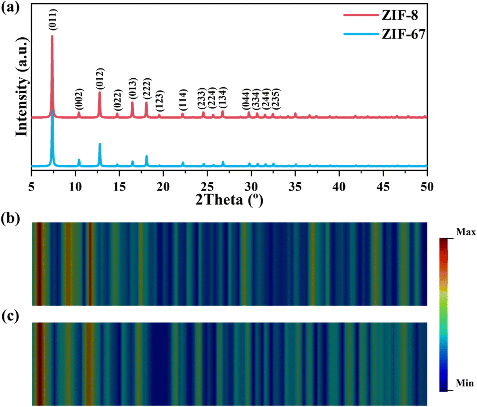Fig. 5 (a) XRD spectra of ZIF-8 and ZIF-67. Class activation maps derived from the CNN-XRD model on (b) ZIF-8 and (c) ZIF-67.

In the context of the ViT model, the learned attention weights can be visualized to investigate the attention allocated to different regions of the input XRD spectra, highlighting the extent to which each input element contributes to the model's decision-making process.^43,44 For each XRD spectrum, a total of 28 attention weight maps can be obtained from the seven encoder layers and four attention heads. Fig. S8† showcases the attention maps for ZIF-8 and ZIF-67 as well as MOF-74 and MOF-199 as these respective XRD spectra are similar to closed primary peaks. Additional examples are available on GitHub. In the first layer, attention disperses across the spectra segments, implying the model's effort to understand the primary patterns. As the ViT-XRD model delves into deeper encoder layers, the attention shifts noticeably to the interrelationships among different spectra segments, leveraging the inherent advantages of the Transformer's attention mechanism. This transition signifies the model's encompassment of various data slices from their simple patterns to complex ones, from a localized relationship to a global one. Close observation found that the attention maps for ZIF-8, ZIF-67, MOF-74, and MOF-199 share similar trends in the first few layers, indicating a broad focus on key features. However, a divergence in attention patterns between ZIF-8/ZIF-67 and MOF-74/MOF-199 becomes evident in the deeper layers. Given that the XRD spectra of MOF-74 and MOF-199 are totally different from those of ZIF-8 and ZIF-67, such divergence highlights the capability of the ViT model to fine-tune its focus on subtle peak differences. The attention mechanism in the Transformer architecture allows the model to capture long-range dependencies and contextual information of the XRD spectra, resulting in higher prediction accuracies.

When it evolves to the last encoder layer (Fig. 6a and b), different attention heads play diverse roles. As for the attention weight map of ZIF-8 and ZIF-67, Heads 1, 3 and 4 exhibit a few obvious vertical patterns, while Head 2 focuses on more specific regions. For instance, Head 1 shows two vertical patterns located at the regions of 5–7.4° and 14.6–17°, corresponding to the (011) plane, (022)/(013) planes, respectively. Head 3 possesses an obvious vertical pattern located at the regions of 9.8–12.2° corresponding to the (022)/(013) planes. Head 4 focuses more on the peaks at 21.8–24.2° for ZIF-8 while the peaks at 7.4–9.8° and 26.6–29° for ZIF-67. As for the specific regions of ZIF-8, in Head 2, the peaks at the 9.8–12.2° region correspond to the (022) plane. For ZIF-67, two large attention weights in Head 1 are related to the peaks of the (011) and (044) planes and the peaks of the (114) and (044)/(344) planes. Head 2 shows the large attention weights to the peaks of the (112) and (114) planes. Head 3 shows large attention weights to the peaks of the (114) and (123) planes, while Head 4 exhibits the large ones to the peaks of the (011) and (233)/(224) planes.

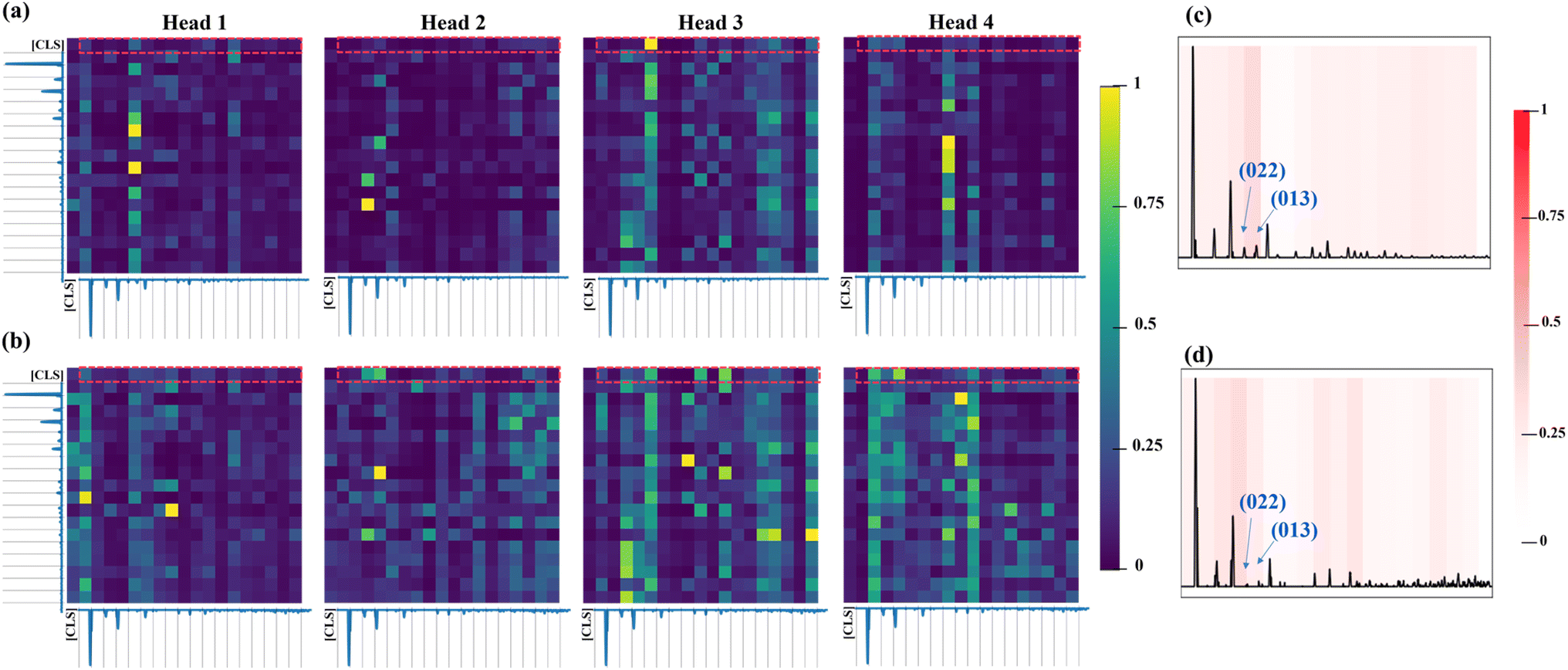Fig. 6 Heat maps of the learned attention weights from the ViT-XRD model's last layer over the XRD spectrum of (a) ZIF-8 and (b) ZIF-67. Normalized attention rollout map of (c) ZIF-8 and (d) ZIF-67.

To directly compare how attention is distributed across the regions of the spectra, an attention rollout map (ARM), as shown in Fig. 6c, is averaged from the first rows of the attention weights from the XRD spectra of ZIF-8 and ZIF-67 (red squares in Fig. 6a and b).⁴⁴ It represents the attention weights of the [CLS] token query over the spectra segments, offering interpretability into the mechanism of a Transformer model on making decisions. The ARM clearly shows that the highest (%7E30%) attention from the VIT-XRD model was concentrated on the (022)/(013) peaks, while the remaining attentions are paid to the other peaks. These results indicated that the ViT model can detect less apparent but potentially relevant peaks by detecting the relevance of the distances and intensity ratios between the peaks when classifying the spectra, thus uncovering the mechanism of how the ViT model can better distinguish very similar spectra than the CNN does.

Reduced 2θ range

Visualization of self-attention weights reveals that the ViT-XRD model focuses more on the initial segments of XRD data for making decisions. This observation prompts us to assess the balance between accuracy and the range of the 2θ angle. This is because narrowing the range will reduce the data amount and subsequently the model training time. Herein, we investigated how narrowing the 2θ range would change the predictive accuracy of the ViT-XRD model (Fig. S9†). The initial 2θ range in 5–50° serves as a baseline. Then it is narrowed to 5–45°, 5–40°, 5–35°, and 5–30° by directly truncating the data points out of these ranges. Subsequently, the ViT-XRD models were retrained using these reduced datasets. In comparison with the original model, the prediction accuracies for Top-1, Top-3, and Top-5 from the retrained models are marginally decreased, but the training time is significantly decreased, highlighting the robustness of the model for rapid classification. For instance, if taking the model trained with 2θ in the range of 5–30° as an example, the Top-1 accuracy slightly decreases from 96.7% to 92%, while the acquisition time is shortened from 11.25 to 6.25 minutes given a scan rate of 4° per minute, which may be further reduced by increasing the scan rate. These results prove that the crucial characteristic features required for MOF classification are predominantly contained within the smaller 2θ ranges.

Transfer learning from XRD to FTIR

The ViT model has exhibited remarkable prediction accuracy in classification of the XRD spectra. Retraining a new model for application in different types of spectra, e.g., FTIR, for a different type of material can be time-consuming, labor-intensive, and often impractical due to the challenges of gathering and curating extensive data. This limitation poses a substantial obstacle to the application of DL in chemical and materials science, where data limitation is an issue. An alternative solution to this issue is to use transfer learning (TL). TL leverages knowledge gained from a source domain and adapts it to another one. This approach has garnered much attention as it mitigates the need for massive datasets and reduces computation. Tian et al. demonstrated a TL strategy to improve the accuracy of classifying Raman spectra trained by limited data.⁴⁵ Another study by Kim and colleagues showcased the universal transferability of a MOFTransformer model.⁴⁶ They achieved this by fine-tuning an already trained model for predictions of diverse MOF properties like gas adsorption, diffusivity, and electronic properties. These accomplishments motivate us to investigate the transferability of our ViT-XRD model to classify another type of spectrum, e.g., FTIR, for a different type of material. The FTIR spectra provide intricate insights into chemical bonding and molecular structures. Each chemical bond possesses distinct light absorption frequencies, resulting in an FTIR spectrum that acts as a molecular “fingerprint”. It can be used to identify unknown substances and quantify specific compounds within mixtures. However, it poses a challenge in analysis and interpretation due to irregular peak shapes, containing various absorptions originating from the distinct functional groups.^47,48 These functional groups are inevitably subjected to varying degrees of influence from nearby molecular features and environmental conditions. Moreover, the presence or absence of a particular functional group is not solely determined by the presence or absence of a single spectral band; it is also by intricate spectral regions. These complexities make the analysis of FTIR time-consuming and error-prone, necessitating the development of powerful and robust analysis techniques to expedite this process.

Given the complexities associated with FTIR analysis, it was chosen as a demo to evaluate the transferability of the ViT-XRD model. Fig. 7a depicts the TL procedure, wherein the ViT-XRD model that was originally trained by the XRD spectra was transferred to classify the experimental FTIR spectra of 3753 organic molecules. They were selected by criteria on the presence of carbon, hydrogen, nitrogen, sulfur, and fluorine atoms while the number of carbon atoms ranges from 6 to 20. Subsequently, these FTIR spectra underwent a series of preprocessing steps, encompassing transmission-to-absorption conversion, wavelength-to-wavenumber conversion, truncation, interpolation, and normalization. It is worth mentioning that neither noise nor background reduction was employed to preprocess the raw FTIR spectra.

Fig. 7 The workflow and results of the transferred ViT model for FTIR classification. (a) Sources of XRD and FTIR spectra and the schematic of transfer learning the ViT-XRD model to the ViT-TL-FTIR model. Prediction accuracies and training times of the ViT-FTIR and ViT-TL-FTIR models (b) as well as the CNN-FTIR and CNN-TL-FTIR models (c) for classifying 3753 molecules.

The transferred ViT model can harness its prior understanding from the XRD spectra to effectively classify the FTIR spectra, even though they differ largely in the spectra characteristics. To train a new ViT model for the FTIR classification by TL, the weights, and biases of the pre-trained ViT-XRD model were used as initial parameters without any subsequent modification or changes of the model components. This model is denoted as ViT-TL-FTIR. As a control, a separate ViT-FTIR model was trained from scratch using the same FTIR spectra. It is worth noting that the configurations with the 10 attention heads and 10 encoders were set for both the ViT-TL-FTIR and ViT-FTIR models. As a control study, a transferred CNN-XRD model, denoted as CNN-TL-FTIR was also trained, while a CNN-FTIR model without TL was developed. Fig. 6b and c show the Top-1, Top-3, and Top-5 prediction accuracies from these models. Generally, the transferred models show enhanced prediction accuracies compared to the non-transferred ones.^45,46 Notably, the ViT-TL-FTIR model outperforms the CNN-TL-FTIR model, with Top-1, Top-3, and Top-5 prediction accuracies of 84%, 94.1%, and 96.7%, respectively, highlighting the inherent advantages of the Transformer architecture, while the ViT-FTIR model affords much lower corresponding accuracies of only 72.5%, 85.4%, and 88.9% (Fig. 7b). Similarly, the CNN-TL-FTIR model delivers prediction accuracies of 50.6%, 66.9% and 73.1% for Top-1, Top-3, and Top-5, respectively, which are higher than those predicted by the CNN-FTIR model (Fig. 7c). But they are respectively lower than those afforded by the ViT-TL-FTIR model, agreeing well with the conclusion that Transformer is superior to CNN for this application.

Furthermore, effects of Embed_dim, augmentation times, and classification categories on the prediction accuracies of the ViT-TL-FTIR model were investigated (Fig. S10–S12†). Fig. S10† shows that the reduction of Embed_dim to 120 decreases the prediction accuracies to 65.5%, 80.2%, and 84.4% for Top-1, Top-3, and Top-5, respectively. A decrease in the augmentation times reduces the prediction accuracies as well as the training time (Fig. S11†). For instance, if the model is trained by data augmented 10 times, the accuracies for Top-1, Top-3, and Top-5 decrease to 68.7%, 83.7%, and 88.5%, and the training time decreases from 420 to 132 seconds. We also investigated the effect of classes (the number of organic molecules) on the model performance. As shown in Fig. S12,† the Top-1 prediction accuracy afforded by the model trained for 500 molecules is 94.4%, which reduces to 84.7% when the number of the molecules increases to 3000. The decrease in the Top-1 prediction accuracy with the increase of classes is common in a classification task.¹⁰

Conclusions

In this study, we demonstrate an interpretable and transferrable ViT model for material classification from their spectra. The ViT model first trained by the XRD spectra of MOFs performs better than the CNN model. Visualization of the attention weight maps illustrates that the self-attention mechanism helps the model to capture long-range dependencies of the tokens in the XRD spectra. Then, the pre-trained ViT-XRD model was successfully transferred to classify the FTIR spectra of organic molecules. Despite the higher characteristic complexity in the FTIR spectra, the transferred models exhibit superior performance to the non-transferred ones. It indicates that by leveraging the TL strategy, the issues of lacking enough high-quality data in the chemical and material fields can be mitigated. This ViT model provides an accurate and interpretable approach to identify materials from their spectral fingerprints, laying a broader platform for analyzing other spectroscopic modalities, such as Raman and NMR. Importantly, the inherent structure of the Transformer models holds great promise for multimodal learning by fusing diverse types of characterization data. Such a multimodal Transformer model, coupled with transferability as demonstrated in this study, would lead to a new route to comprehensive structure–property analysis.

Methods

Theoretical and experimental XRD data: collection and processing

A total of 2000 theoretical XRD spectra in the Crystallographic Information File (CIF) were sourced from an open-source database of the Cambridge Crystallographic Data Centre (CCDC). Then, all CIFs were converted in a batch mode to a tab-separated format using Mercury software for subsequent data processing. To collect the experimental XRD, ten MOFs (ZIF-7, ZIF-8, ZIF-9, ZIF-67, ZIF-71, ZIF-90, MOF-2, MOF-5, MOF-74 and MOF-199) were synthesized by three common methods, resulting in a total of thirty MOF samples.¹⁰ Then experimental XRD spectra were collected from these samples using a Bruker D8 Advance XRD. The spectra underwent processing procedures of noise reduction and background subtraction and then were augmented. Details are explained in ESI Note S2.† To maintain consistency, all XRD spectra were truncated to the same 2θ range of 5–50°, and then rescaled to a range of 0–1.

FTIR data collection and processing

A total of 3753 organic molecules were sourced from the National Institute for Science and Technology (NIST) Chemistry WebBook. Specifically, the molecules that contain 6–20 carbon atoms, hydrogen, nitrogen, sulfur, and fluorine were selected. These FTIR spectra were standardized to the absorption type with the same wavenumber unit. Subsequently, a three-step data processing by truncation, interpolation, and intensity normalization was employed to ensure a constant wavenumber in the same range of 700–3500 and a standardized absorption intensity in the range of 0–1. Note that they did not undergo noise or background reduction. Note that among the 5–10 FTIR spectra for each molecule, one spectrum was designed as the test set. The remaining ones were randomly selected for augmentation to a total of 50 spectra. These augmented datasets were subsequently partitioned into training and validation subsets with a ratio of 4 : 1.

Model training

NB, KNN, LR, RF, XGB, CNN, and ViT were trained. A grid-search strategy was applied to find the optimal hyperparameters. To prevent overfitting, an early stopping strategy was implemented when training the CNN and ViT models. The training was terminated prematurely if it surpassed a patience level of 3 epochs without a significant decrease in the loss. Unless specified, for each model, the training was replicated ten times to obtain the mean and standard deviations of the prediction accuracies. The model performance was evaluated using Top-N accuracy on the test datasets. In detail, Top-1 accuracy refers to the ViT model's capability to correctly rank an MOF sample at the first position. Meanwhile, Top-3 and Top-5 accuracies assess the model's accuracy in ranking the sample within the top three and top five positions, respectively.¹⁰ All computations were conducted on a desktop equipped with an Intel Core i7-12700K processor, an NVIDIA GeForce 2080 GPU, and 64 GB of RAM, running on the Ubuntu 22.04.2 operating system. The codes were implemented using Python 3.7.9. For data processing, we utilized NumPy version 1.19.2 and Pandas version 1.2.1. The data processing and analysis on the traditional ML models were undertaken using Scikit-learn 1.0.2. The CNN model was constructed using the TensorFlow 2.2.0 framework, while the ViT model was built using PyTorch 1.13.1+cu117.

Heatmap

ARM and CAM for ViT-XRD and CNN-XRD models, respectively, were plotted. For the ARM, the attention weights associated with the ‘CLS’ token were extracted from each attention head in the last layer of the Transformer encoder. These attention weights indicate the importance of different positions in the input sequence relative to the ‘CLS’ token. These weights were averaged across all attention heads to create a composite attention vector, which illustrates the cumulative attention in the model allocated to the CLS token. Each composite vector was mapped to the corresponding XRD spectrum. The CAM was plot by utilizing the output of the last convolutional layer of the CNN-XRD model. Specifically, we took the weights from the fully connected layer and performed a matrix multiplication with the feature maps from the last convolutional layer.

Data availability

All codes are publicly available at https://github.com/linresearchgroup/ViT_Materials_Spectra. For the source data, the theoretical XRD spectra are available from the CCDC. The experimental FTIR spectra can be sourced from the NIST WebBook and are copyrighted by NIST. Additional attention maps for the XRD spectra of other MOFs are summarized in (https://github.com/linresearchgroup/ViT_Materials_Spectra/tree/main/Visualization). Additional data can be made available from the corresponding author upon request.

Author contributions

Z. C. designed and implemented data collection and preprocessing, model training and testing, and data analysis. Y. X. performed supervision of material synthesis and characterization, and machine learning algorithm development. Y. W. provided the suggestion for the analysis of FTIR spectra. J. L. conceived the project, managed the research progress, and provided regular guidance. Z. C. and Y. X. drafted the manuscript which was thoroughly revised by J. L. S. T. and Y. L. offered regular feedback during the project implementation. S. T. made a minor revision of the manuscript. All authors commented and agreed on the final version of the manuscript.

Conflicts of interest

The authors declare no competing interests.

Acknowledgements

J. L. thanks the financial support from the National Science Foundation (award number: 2154428), U.S. Army Corps of Engineers, ERDC (grant number: W912HZ-21-2-0050), DOE National Energy Technology Laboratory (award number: DE-FE0031988), and Sony Research Award Program (2020). We also acknowledge help from Kotaro Satori at Sony Semiconductor Solutions Corporation.

References

1. J. Meckling, J. E. Aldy, M. J. Kotchen, S. Carley, D. C. Esty, P. A. Raymond, B. Tonkonogy, C. Harper, G. Sawyer and J. Sweatman, Busting the myths around public investment in clean energy, Nat. Energy, 2022, 7, 563–565.
2. D. P. Tabor, L. M. Roch, S. K. Saikin, C. Kreisbeck, D. Sheberla, J. H. Montoya, S. Dwaraknath, M. Aykol, C. Ortiz, H. Tribukait, C. Amador-Bedolla, C. J. Brabec, B. Maruyama, K. A. Persson and A. Aspuru-Guzik, Accelerating the discovery of materials for clean energy in the era of smart automation, Nat. Rev. Mater., 2018, 3, 5–20.
3. P. S. Gromski, A. B. Henson, J. M. Granda and L. Cronin, How to explore chemical space using algorithms and automation, Nat. Rev. Chem, 2019, 3, 119–128.
4. Y. Shi, P. L. Prieto, T. Zepel, S. Grunert and J. E. Hein, Automated Experimentation Powers Data Science in Chemistry, Acc. Chem. Res., 2021, 54, 546–555.
5. Y. Xie, K. Sattari, C. Zhang and J. Lin, Toward autonomous laboratories: Convergence of artificial intelligence and experimental automation, Prog. Mater. Sci., 2023, 132, 101043.
6. H. Wang, T. Fu, Y. Du, W. Gao, K. Huang, Z. Liu, P. Chandak, S. Liu, P. Van Katwyk, A. Deac, A. Anandkumar, K. Bergen, C. P. Gomes, S. Ho, P. Kohli, J. Lasenby, J. Leskovec, T.-Y. Liu, A. Manrai, D. Marks, B. Ramsundar, L. Song, J. Sun, J. Tang, P. Veličković, M. Welling, L. Zhang, C. W. Coley, Y. Bengio and M. Zitnik, Scientific discovery in the age of artificial intelligence, Nature, 2023, 620, 47–60.
7. Y. Xie, C. Zhang, X. Hu, C. Zhang, S. P. Kelley, J. L. Atwood and J. Lin, Machine Learning Assisted Synthesis of Metal–Organic Nanocapsules, J. Am. Chem. Soc., 2020, 142, 1475–1481.
8. Y. Dong, C. Wu, C. Zhang, Y. Liu, J. Cheng and J. Lin, Bandgap prediction by deep learning in configurationally hybridized graphene and boron nitride, npj Comput. Mater., 2019, 5, 26.
9. F. Oviedo, Z. Ren, S. Sun, C. Settens, Z. Liu, N. T. P. Hartono, S. Ramasamy, B. L. DeCost, S. I. P. Tian, G. Romano, A. Gilad Kusne and T. Buonassisi, Fast and interpretable classification of small X-ray diffraction datasets using data augmentation and deep neural networks, npj Comput. Mater., 2019, 5, 60.
10. H. Wang, Y. Xie, D. Li, H. Deng, Y. Zhao, M. Xin and J. Lin, Rapid Identification of X-ray Diffraction Patterns Based on Very Limited Data by Interpretable Convolutional Neural Networks, J. Chem. Inf. Model., 2020, 60, 2004–2011.
11. J. A. Fine, A. A. Rajasekar, K. P. Jethava and G. Chopra, Spectral deep learning for prediction and prospective validation of functional groups, Chem. Sci., 2020, 11, 4618–4630.
12. A. Angulo, L. Yang, E. S. Aydil and M. A. Modestino, Machine learning enhanced spectroscopic analysis: towards autonomous chemical mixture characterization for rapid process optimization, Digital Discovery, 2022, 1, 35–44.
13. T.-Y. Huang and J. C. C. Yu, Development of Crime Scene Intelligence Using a Hand-Held Raman Spectrometer and Transfer Learning, Anal. Chem., 2021, 93, 8889–8896.
14. X. Fan, Y. Wang, C. Yu, Y. Lv, H. Zhang, Q. Yang, M. Wen, H. Lu and Z. Zhang, A Universal and Accurate Method for Easily Identifying Components in Raman Spectroscopy Based on Deep Learning, Anal. Chem., 2023, 95, 4863–4870.
15. A. D. Melnikov, Y. P. Tsentalovich and V. V. Yanshole, Deep Learning for the Precise Peak Detection in High-Resolution LC-MS Data, Anal. Chem., 2020, 92, 588–592.
16. D. A. Boiko, K. S. Kozlov, J. V. Burykina, V. V. Ilyushenkova and V. P. Ananikov, Fully Automated Unconstrained Analysis of High-Resolution Mass Spectrometry Data with Machine Learning, J. Am. Chem. Soc., 2022, 144, 14590–14606.
17. Z. Zhao, X. Wu and H. Liu, Vision transformer for quality identification of sesame oil with stereoscopic fluorescence spectrum image, Lebensm.-Wiss. Technol., 2022, 158, 113173.
18. A. Vaswani, N. Shazeer, N. Parmar, J. Uszkoreit, L. Jones, A. N. Gomez, L. Kaiser and I. Polosukhin, Attention Is All You Need, arXiv, 2017, preprint, arXiv:1706.03762,  DOI:10.48550/arXiv.1706.03762.
19. J. Devlin, M.-W. Chang, K. Lee and K. Toutanova: Pre-training of Deep Bidirectional Transformers for Language Understanding, arXiv, 2018, preprint, arXiv:1810.04805,  DOI:10.48550/arXiv.1810.04805.
20. T. B. Brown, B. Mann, N. Ryder, M. Subbiah, J. Kaplan, P. Dhariwal, A. Neelakantan, P. Shyam, G. Sastry, A. Askell, S. Agarwal, A. Herbert-Voss, G. Krueger, T. Henighan, R. Child, A. Ramesh, D. M. Ziegler, J. Wu, C. Winter, C. Hesse, M. Chen, E. Sigler, M. Litwin, S. Gray, B. Chess, J. Clark, C. Berner, S. McCandlish, A. Radford, I. Sutskever and D. Amodei, Language Models are Few-Shot Learners, arXiv, 2020, preprint, arXiv:2005.14165,  DOI:10.48550/arXiv.2005.14165.
21. A. Chowdhery, S. Narang, J. Devlin, M. Bosma, G. Mishra, A. Roberts, P. Barham, H. W. Chung, C. Sutton, S. Gehrmann, P. Schuh, K. Shi, S. Tsvyashchenko, J. Maynez, A. Rao, P. Barnes, Y. Tay, N. Shazeer, V. Prabhakaran, E. Reif, N. Du, B. Hutchinson, R. Pope, J. Bradbury, J. Austin, M. Isard, G. Gur-Ari, P. Yin, T. Duke, A. Levskaya, S. Ghemawat, S. Dev, H. Michalewski, X. Garcia, V. Misra, K. Robinson, L. Fedus, D. Zhou, D. Ippolito, D. Luan, H. Lim, B. Zoph, A. Spiridonov, R. Sepassi, D. Dohan, S. Agrawal, M. Omernick, A. M. Dai, T. Sankaranarayana Pillai, M. Pellat, A. Lewkowycz, E. Moreira, R. Child, O. Polozov, K. Lee, Z. Zhou, X. Wang, B. Saeta, M. Diaz, O. Firat, M. Catasta, J. Wei, K. Meier-Hellstern, D. Eck, J. Dean, S. Petrov and N. Fiedel, PaLM: Scaling Language Modeling, with Pathways, arXiv, 2022, preprint, arXiv:2204.02311,  DOI:10.48550/arXiv.2204.02311.
22. H. Touvron, T. Lavril, G. Izacard, X. Martinet, M.-A. Lachaux, T. Lacroix, B. Rozière, N. Goyal, E. Hambro, F. Azhar, A. Rodriguez, A. Joulin, E. Grave and G. Lample, LLaMA: Open and Efficient Foundation Language Models, arXiv, 2023, preprint, arXiv:2302.13971,  DOI:10.48550/arXiv.2302.13971.
23. K. Singhal, S. Azizi, T. Tu, S. S. Mahdavi, J. Wei, H. W. Chung, N. Scales, A. Tanwani, H. Cole-Lewis, S. Pfohl, P. Payne, M. Seneviratne, P. Gamble, C. Kelly, A. Babiker, N. Schärli, A. Chowdhery, P. Mansfield, D. Demner-Fushman, B. Agüera y Arcas, D. Webster, G. S. Corrado, Y. Matias, K. Chou, J. Gottweis, N. Tomasev, Y. Liu, A. Rajkomar, J. Barral, C. Semturs, A. Karthikesalingam and V. Natarajan, Large language models encode clinical knowledge, Nature, 2023, 620, 172–180.
24. P. Schwaller, T. Laino, T. Gaudin, P. Bolgar, C. A. Hunter, C. Bekas and A. A. Lee, Molecular Transformer: A Model for Uncertainty-Calibrated Chemical Reaction Prediction, ACS Cent. Sci., 2019, 5, 1572–1583.
25. S. Chithrananda, G. Grand and B. Ramsundar, ChemBERTa: Large-Scale Self-Supervised Pretraining for Molecular Property Prediction, arXiv, 2020, preprint, arXiv:2010.09885,  DOI:10.48550/arXiv.2010.09885.
26. V. Mann and V. Venkatasubramanian, Predicting chemical reaction outcomes: A grammar ontology-based transformer framework, AIChE J., 2021, 67, e17190.
27. T. Jin, Q. Zhao, A. B. Schofield and B. M. Savoie, Machine Learning Models Capable of Chemical Deduction for Identifying Reaction Products, ChemRxiv, 2023, preprint,  DOI:10.26434/chemrxiv-2023-l6lzp.
28. H. Park, Y. Kang and J. Kim, PMTransformer: Universal Transfer Learning and Cross-material Few-shot Learning in Porous Materials, ChemRxiv, 2023, preprint,  DOI:10.26434/chemrxiv-2023-979mt.
29. D. Elser, F. Huber and E. Gaquerel, Mass2SMILES: deep learning based fast prediction of structures and functional groups directly from high-resolution MS/MS spectra, bioRxiv, 2023, preprint,  DOI:10.1101/2023.07.06.547963.
30. M. Alberts, F. Zipoli and A. C. Vaucher, Learning the Language of NMR: Structure Elucidation from NMR spectra using Transformer Models, ChemRxiv, 2023, preprint,  DOI:10.26434/chemrxiv-2023-8wxcz.
31. A. Young, B. Wang and H. Röst: Tandem Mass Spectrum Prediction for Small Molecules using Graph Transformers, arXiv, 2021, preprint, arXiv:2111.04824,  DOI:10.48550/arXiv.2111.04824.
32. B. Liu, K. Liu, X. Qi, W. Zhang and B. Li, Classification of deep-sea cold seep bacteria by transformer combined with Raman spectroscopy, Sci. Rep., 2023, 13, 3240.
33. B. L. Thomsen, J. B. Christensen, O. Rodenko, I. Usenov, R. B. Grønnemose, T. E. Andersen and M. Lassen, Accurate and fast identification of minimally prepared bacteria phenotypes using Raman spectroscopy assisted by machine learning, Sci. Rep., 2022, 12, 16436.
34. Y.-M. Tseng, K.-L. Chen, P.-H. Chao, Y.-Y. Han and N.-T. Huang, Deep Learning–Assisted Surface-Enhanced Raman Scattering for Rapid Bacterial Identification, ACS Appl. Mater. Interfaces, 2023, 15, 26398–26406.
35. T. Zhang, S. Chen, A. Wulamu, X. Guo, Q. Li and H. Zheng, TransG-net: transformer and graph neural network based multi-modal data fusion network for molecular properties prediction, Appl. Intell., 2023, 53, 16077–16088.
36. S. Goldman, J. Xin, J. Provenzano and C. W. Coley: Chemical formula inference from tandem mass spectra, arXiv, 2023, preprint, arXiv:2307.08240,  DOI:10.48550/arXiv.2307.08240.
37. C. Shorten and T. M. Khoshgoftaar, A survey on Image Data Augmentation for Deep Learning, J. Big Data, 2019, 6, 60.
38. P. Nikolaev, D. Hooper, F. Webber, R. Rao, K. Decker, M. Krein, J. Poleski, R. Barto and B. Maruyama, Autonomy in materials research: a case study in carbon nanotube growth, npj Comput. Mater., 2016, 2, 16031.
39. M. Blanco, J. Coello, H. Iturriaga, S. Maspoch and C. Pérez-Maseda, Determination of polymorphic purity by near infrared spectrometry, Anal. Chim. Acta, 2000, 407, 247–254.
40. X. Fan, W. Ming, H. Zeng, Z. Zhang and H. Lu, Deep learning-based component identification for the Raman spectra of mixtures, Analyst, 2019, 144, 1789–1798.
41. L. Van der Maaten and G. Hinton, Visualizing Data using t-SNE, J. Mach. Learn. Res., 2008, 9, 2579–2605.
42. B. Zhou, A. Khosla, A. Lapedriza, A. Oliva and A. Torralba, Learning Deep Features for Discriminative Localization, arXiv, 2015, preprint, arXiv:1512.04150,  DOI:10.48550/arXiv.1512.04150.
43. J. Vig, A Multiscale Visualization of Attention in the Transformer Model, arXiv, 2019, preprint, arXiv:1906.05714,  DOI:10.48550/arXiv.1906.05714.
44. S. Abnar and W. Zuidema, Quantifying Attention Flow in Transformers, arXiv, 2020, preprint, arXiv:2005.00928,  DOI:10.48550/arXiv.2005.00928.
45. R. Zhang, H. Xie, S. Cai, Y. Hu, G.-k. Liu, W. Hong and Z.-q. Tian, Transfer-learning-based Raman spectra identification, J. Raman Spectrosc., 2020, 51, 176–186.
46. Y. Kang, H. Park, B. Smit and J. Kim, A multi-modal pre-training transformer for universal transfer learning in metal–organic frameworks, Nat. Mach. Intell., 2023, 5, 309–318.
47. Z. Wang, X. Feng, J. Liu, M. Lu and M. Li, Functional groups prediction from infrared spectra based on computer-assist approaches, Microchem. J., 2020, 159, 105395.
48. F. Zhang, R. Zhang, W. Wang, W. Yang, L. Li, Y. Xiong, Q. Kang and Y. Du, Ridge regression combined with model complexity analysis for near infrared (NIR) spectroscopic model updating, Chemom. Intell. Lab. Syst., 2019, 195, 103896.

---

Footnote

† Electronic supplementary information (ESI) available. See DOI: https://doi.org/10.1039/d3dd00198a

---