 Open Access Article
iSIM: instant similarity†
Kenneth
López-Pérez
,
Taewon D.
Kim
and
Ramón Alain
Miranda-Quintana
 *
*
Department of Chemistry and Quantum Theory Project, University of Florida, Gainesville, Florida 32611, USA. E-mail: quintana@chem.ufl.edu
First published on 7th May 2024
Abstract
The quantification of molecular similarity has been present since the beginning of cheminformatics. Although several similarity indices and molecular representations have been reported, all of them ultimately reduce to the calculation of molecular similarities of only two objects at a time. Hence, to obtain the average similarity of a set of molecules, all the pairwise comparisons need to be computed, which demands a quadratic scaling in the number of computational resources. Here we propose an exact alternative to this problem: iSIM (instant similarity). iSIM performs comparisons of multiple molecules at the same time and yields the same value as the average pairwise comparisons of molecules represented by binary fingerprints and real-value descriptors. In this work, we introduce the mathematical framework and several applications of iSIM in chemical sampling, visualization, diversity selection, and clustering.
Introduction
Molecular fingerprints are one of the most common representations of compounds in cheminformatics. The simplest version of fingerprints is binary vectors, where the presence of a structural feature is represented by a 1 and its absence by a 0.1 Another popular representation is molecular descriptors, which correspond to useful numbers that encode information about a molecule; commonly they can be calculated from graph theory, quantum chemistry, and topological or experimental methods, to mention some sources.2 Despite their apparent differences, both descriptors and fingerprints can be used to calculate the similarity between two molecules. From a mathematical point of view, a similarity index is a metric that measures how “related” two points are in chemical space.3 Multiple similarity measurements have been reviewed and analysed, with the well-known Tanimoto coefficient (T)4,5 being the usual go-to in the cheminformatics community.6 The main point of calculating similarity measurements lies in the “molecular similarity principle”: similar molecules have similar properties/activities.7 This powerful idea is at the core of virtual screening,8–11 hit selection,12 QSAR/QSPR modeling,13,14 many chemical space exploration methods,15,16 activity landscape description,17,18 diversity selection,19 clustering,20,21 and many more applications.Given the fundamental role that molecular similarity plays in drug design,22 activity studies23,24 and, more recently, in ML and AI pipelines,25–27 it is not surprising that a lot of effort has been devoted to increase the efficiency of these calculations. For instance, KD-trees28,29 and Ball-trees30 can be used to speed up similarity searches, while packages like FPSim2 (ref. 31) and chemfp32 are superbly optimized. In most cases, the common way of quantifying similarity is by comparing two molecules. The typical way of calculating a library's similarity/diversity is calculating the average similarity of all the possible comparisons in the library, which is a computationally costly O(N2) step. At best, KD-trees can be used to estimate library diversity in an algorithm with N![[thin space (1/6-em)]](https://www.rsc.org/images/entities/char_2009.gif) log
log![[thin space (1/6-em)]](https://www.rsc.org/images/entities/char_2009.gif) N complexity.33 This problem has received attention from the cheminformatics community, perhaps more notably in the work of Willet et al.34,35 For example, these authors proposed an O(N) approximation to the cosine similarity, but despite its appeal, it was not possible to generalize it to other similarity indices.
N complexity.33 This problem has received attention from the cheminformatics community, perhaps more notably in the work of Willet et al.34,35 For example, these authors proposed an O(N) approximation to the cosine similarity, but despite its appeal, it was not possible to generalize it to other similarity indices.
Motivated by this problem, our group recently developed the concept of extended similarity.36,37 Extended similarity performs the comparison of all the molecules in a set at the same time and yields a similarity metric for the whole set. Briefly, for a matrix of size N × M, where M is the size of the fingerprint or number of molecular descriptors and N the number of molecules in a set, the first step is to sum the elements column-wise, resulting in a vector, K = [k1, k2, …, kM]. Each column sum, kq, can be used to classify the column when it is compared to a threshold in the following way: (i) if 2kq − N > γ it will be a 1-similarity column, (ii) if N − 2kq > γ it will be a 0-similarity column, (iii) otherwise it will count as dissimilarity. Then, using Δkq = |2kq − N| as an independent variable a weighting function should be used to consider partial similarity and dissimilarity, and the function should be positive and increasing. Now the variables of any similarity metric can be transformed using the sum of the weighted or non-weighted counters. The major advantage of extended similarity is that it calculates a similarity metric for the whole set much more efficiently than by using the traditional pairwise comparisons, with this calculation now scaling as O(N).36,37
The notion of calculating average similarity values over a set of molecules has proven to be particularly powerful over several cheminformatics tasks. For example, extended similarity has been applied to several problems like diversity selection,37,38 molecular dynamics simulations,39,40 library diversity studies,41–43 activity cliffs,44 descriptor selection for the QSAR/QSPR model,45 fingerprint evaluations,46 and chemical space visualization.47 However, despite these advantages, there are some drawbacks like the need for a coincidence threshold analysis to determine the best similarity/dissimilarity separation and a different numeric value than the pairwise comparisons. These limitations inspired this work where we show the mathematical framework, analysis, and cheminformatics applications of iSIM, an “instantaneous” similarity measurement for binary fingerprints and molecular descriptors that yields virtually the same value as the average pairwise similarity comparisons in a linear scaling with the number of observations.
Theory
Binary representations
Comparisons of molecular fingerprints are based on three key indicators: the number of times there is a coincidence of two “on” bits between the fingerprints (denoted by a), the number of times there is a coincidence of two “off” bits between the fingerprints (denoted by d), and the mismatches between the fingerprints, when one bit is “on” and the other is “off” (denoted by b + c). With these ingredients one can propose a plethora of similarity indices, which could be interpreted as such as long as they are monotonically increasing functions of a and d, and monotonically decreasing functions of b + c. Here, we will be concerned mainly with the Russel–Rao (RR),48 Tanimoto (T),4,5 and Sokal–Michener (SM)49 indices: | (1) |
 | (2) |
 | (3) |
(Notice that, trivially, RR ≤ T ≤ SM.)
The very definition of, say, a seems to imply that when we have N molecules, we need to consider the  distinct pairs to check the coincidence or not of on bits. However, it is possible to access the same information in far fewer operations. The first step is to arrange all the fingerprints in a matrix, with each fingerprint corresponding to a row. Then, we just need to find the sum of each column, which generates the same vector described before. However, the key insight now is to note that the k's are all that we need to calculate the number of times we will have coincidence or not of any type of bit. For instance, there will be
  instances in which two on bits will coincide in column q. Likewise, there will be
  coincidences of off bits. Finally, the number of mismatches is kq(N − kq). It is natural then to make the following identification (with the sums running over all bit positions):
 | (4) |
 | (5) |
 | (6) |
With this, we have everything in place to define the instantaneous similarity (iSIM) versions of the previously discussed indices, iRR, iT, and iSM, as:
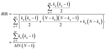 | (7) |
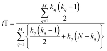 | (8) |
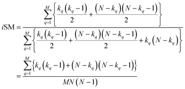 | (9) |
The case of iRR and iSM is special, because a + b + c + d = M, the denominators in eqn (1) and (3), are always constant, equal to the number of bits in the fingerprints (a fact that we explicitly use in the 2nd, simpler, form of the iRR and iSM indices shown above). Then, we can interpret eqn (7) and (9) as effectively combining the RR and SM similarities over independent bit positions. Given the constant-denominator characteristic, it is then easy to see that the iSIM version of these indices will provide the exact average of all the pairwise RR and SM values over the given set, but at only O(N) cost. iT, on the other hand, will not in general give exactly the same value as the average of the pairwise Tanimoto calculations. Once again, the key is that the T denominator is not the same for arbitrary pairs of fingerprints. In this case, we can interpret iT as an O(N) mediant approximation50,51 to the O(N2) average. Despite this simplification, as shown below, iT still provides superb estimates for the pairwise average over a varied set of conditions.
Real-value representations
The previous results are promising, so it is certainly desirable to extend them to more general types of molecular representations. Here, we show how this can be done for vectors of real (in principle, continuous) values. The key insight is to use inner products between the molecular “vectors” instead of the more limited a, d, and b + c indicators used in the binary case. To do this we will focus on the case where the ith molecule, X(i), is represented by a vector of descriptors |X(i)〉 = [x1(i), x2(i), …, xM(i)]. Without losing any generality, these vectors are considered to be normalized: ∀i, q: 0 ≤ xq(i) ≤ 1. The main motivation behind the focus on normalized descriptors is that we can then easily define the “flipped” representation of a molecule, |![[X with combining tilde]](https://www.rsc.org/images/entities/i_char_0058_0303.gif) (i), as the real-value equivalent of flipping the bits of a binary representation, that is: |
(i), as the real-value equivalent of flipping the bits of a binary representation, that is: |![[X with combining tilde]](https://www.rsc.org/images/entities/i_char_0058_0303.gif) (i)〉 = [1 − x1(i), 1 − x2(i), …, 1 − xM(i)]. In terms of inner products, the previously analyzed indices can be written as:
(i)〉 = [1 − x1(i), 1 − x2(i), …, 1 − xM(i)]. In terms of inner products, the previously analyzed indices can be written as: | (10) |
 | (11) |
 | (12) |
Notice that, for simplicity, we have directly used the fact that the denominators of the RR and SM indices are constant and equal to the total length of the molecular vectors, M.
Once again, the way of writing eqn (10)–(12) seems to suggest that calculating the average of all the RR, T, or SM comparisons demands O(N2). However, we can actually calculate the sum of all the involved inner products in O(N) (albeit with a larger overhead compared to the binary case).
First, for the inner products between the molecular representations, we have:
 | (13) |
Then, for the relevant inner products appearing in eqn (10)–(12):
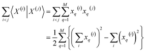 | (14) |
 | (15) |
From these expressions, it is clear that we can follow a similar route to the one taken for the binary input. First, we need to arrange all the molecular vectors in a matrix X. Then, we need to generate some related matrices: (a) the “flipped” matrix ![[X with combining tilde]](https://www.rsc.org/images/entities/i_char_0058_0303.gif) = 1 − X, (b) the Hadamard (element-wise) squares of these matrices, X2 and
= 1 − X, (b) the Hadamard (element-wise) squares of these matrices, X2 and ![[X with combining tilde]](https://www.rsc.org/images/entities/i_char_0058_0303.gif) 2. That is, if the element in row i and column q in X is given by xq(i), then the corresponding elements of matrices
2. That is, if the element in row i and column q in X is given by xq(i), then the corresponding elements of matrices ![[X with combining tilde]](https://www.rsc.org/images/entities/i_char_0058_0303.gif) , X2, and
, X2, and ![[X with combining tilde]](https://www.rsc.org/images/entities/i_char_0058_0303.gif) 2 will be 1 − xq(i), (xq(i))2, and [1 − xq(i)]2, respectively. It is important to remark that since we are only taking element-wise products, generating these auxiliary matrices will only demand O(N) operations. Then, the sum of the columns of matrices X and
2 will be 1 − xq(i), (xq(i))2, and [1 − xq(i)]2, respectively. It is important to remark that since we are only taking element-wise products, generating these auxiliary matrices will only demand O(N) operations. Then, the sum of the columns of matrices X and ![[X with combining tilde]](https://www.rsc.org/images/entities/i_char_0058_0303.gif) gives vectors with components
gives vectors with components  and
and  , respectively. On the other hand, the sum of the columns for the Hadamard squares gives the factors
  and
and  . These are all the ingredients necessary to calculate the real-value iSIM similarity indices:
 | (16) |
 | (17) |
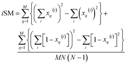 | (18) |
Once again, iRR and iSM provide the same exact results as the average of all the pairwise comparisons, due to the convenient constant denominators. For iT, this is just a median-like approximation but, as will be illustrated below with different numerical tests, eqn (17) provides an excellent approximation to the O(N2) result.
Datasets
10![[thin space (1/6-em)]](https://www.rsc.org/images/entities/char_2009.gif) 000 random datasets were generated, with the number of fingerprints ranging from 100 to 1000 and the size of the fingerprints ranging from 166 to 2048. For the binary case, to ensure that the datasets covered the complete range of the similarity index domains, each dataset was randomly biased to have different proportions of ones and zeros. The code to generate the random sets is shown in iSIM_simulated_fps.ipynb. The generation of the sets employs functions from numpy52 1.24.2 and random53 python packages.
000 random datasets were generated, with the number of fingerprints ranging from 100 to 1000 and the size of the fingerprints ranging from 166 to 2048. For the binary case, to ensure that the datasets covered the complete range of the similarity index domains, each dataset was randomly biased to have different proportions of ones and zeros. The code to generate the random sets is shown in iSIM_simulated_fps.ipynb. The generation of the sets employs functions from numpy52 1.24.2 and random53 python packages.
For testing on real libraries, 30 ChEMBL29 curated datasets by van Tilborg et al.54 were used (sets are available on https://github.com/molML/MoleculeACE/tree/main/MoleculeACE/Data/benchmark_data/old). The datasets had been curated by the authors using the default RDKIT sanitation and outlier exclusion based on bioactivity.54 Details of the set's size and corresponding targets are shown in Table S1.† The sets consisted of three binary fingerprint types, generated using RDKit:55 RDKIT55 (M = 2048), MACCS56 (M = 167) and ECFP4 (ref. 57) (M = 1024). All the continuous and discrete descriptors offered by the RDKit Descriptors55 module were computed, descriptors with calculation errors or nan values were dropped for a total of 208 descriptors (for the full list, see the ESI†). Min max normalization was used prior to iSIM calculations.
Results
Average similarity
Our first tests were oriented towards checking the correspondence between the iSIM results and the average of the pairwise comparisons over a large number of libraries. For this, we used the 10![[thin space (1/6-em)]](https://www.rsc.org/images/entities/char_2009.gif) 000 randomly generated libraries described in the previous section. As can be seen in Fig. 1, the iSIM results perfectly reproduce the more computationally demanding standard comparisons. In our previous contributions, we had only focused on the relation between the previously extended similarity results and the pairwise metrics as far as the ability of the extended indices to preserve the ranking of the comparisons (see, for example, Fig. 7 in ref. 23). The test presented in Fig. 1 is much more demanding, because we are comparing the similarity values obtained from both approaches. As noted in the Theory section, we expected the iRR and iSM results to be (analytically) identical to the pairwise averages. Even more remarkable, we see that iT provides a superb estimate for the O(N2) averages. This behavior is also observed over real datasets. In Fig. 2 we show a similar comparison, but now over 30 CHEMBL libraries, each represented by three different types of fingerprints. Fig. S1 and S2† include the same comparisons with more similarity index formulas that iSIM can be applied to.
000 randomly generated libraries described in the previous section. As can be seen in Fig. 1, the iSIM results perfectly reproduce the more computationally demanding standard comparisons. In our previous contributions, we had only focused on the relation between the previously extended similarity results and the pairwise metrics as far as the ability of the extended indices to preserve the ranking of the comparisons (see, for example, Fig. 7 in ref. 23). The test presented in Fig. 1 is much more demanding, because we are comparing the similarity values obtained from both approaches. As noted in the Theory section, we expected the iRR and iSM results to be (analytically) identical to the pairwise averages. Even more remarkable, we see that iT provides a superb estimate for the O(N2) averages. This behavior is also observed over real datasets. In Fig. 2 we show a similar comparison, but now over 30 CHEMBL libraries, each represented by three different types of fingerprints. Fig. S1 and S2† include the same comparisons with more similarity index formulas that iSIM can be applied to.
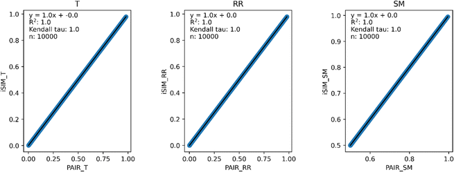 | ||
Fig. 1 iSIM vs. average pairwise similarity for 10![[thin space (1/6-em)]](https://www.rsc.org/images/entities/char_2009.gif) 000 randomly generated libraries. Molecules are represented by binary fingerprints. 000 randomly generated libraries. Molecules are represented by binary fingerprints. | ||
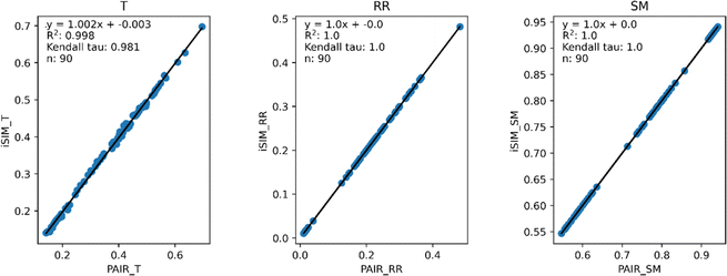 | ||
| Fig. 2 iSIM vs. average pairwise similarity for 30 CHEMBL libraries. Molecules are represented by binary MACCS, RDKit, and ECFP4 (binary) fingerprints. | ||
Fig. 3 and 4 present the equivalent results, but for molecules represented by (normalized) descriptors (e.g., continuous real values). Once again, iRR and iSM show a perfect agreement both for the randomly generated and for the real data. The median approximation in iT is also remarkably robust over continuous data, essentially operating at as close a level as for the binary fingerprints.
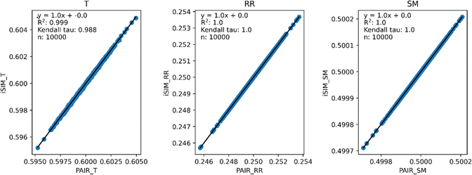 | ||
Fig. 3 iSIM vs. average pairwise similarity for 10![[thin space (1/6-em)]](https://www.rsc.org/images/entities/char_2009.gif) 000 randomly generated libraries. Molecules are represented by random generated fingerprints with continuous normalized descriptors. 000 randomly generated libraries. Molecules are represented by random generated fingerprints with continuous normalized descriptors. | ||
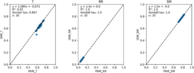 | ||
| Fig. 4 iSIM vs. average pairwise similarity for 30 CHEMBL libraries. Molecules are represented by 208 RDKIT continuous and discrete numerical normalized descriptors. | ||
Local analysis of molecular libraries
Pick a molecule and add it to the selected set. (This is usually done at random, but in order to increase the reproducibility of our results, in all cases we start from the medoid of the set.)
At every step, pick the molecule that will result in the lowest iSIM for the selected set.
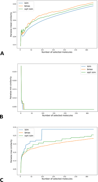
As shown in Fig. 6A, this simple recipe leads to more diverse sub-sets than the popular MaxMin diversity selection algorithm.58,59 There, we tested the performance of these algorithms over the CHEMBL214 library, corresponding to the 5-HT1a receptor.54 We selected a library with 3317 molecules (represented using RDKIT fingerprints), and we monitored the process of selecting up to the 10% most diverse compounds. (The general trends observed for this library were corroborated for other libraries, similarity indices, and fingerprint types; see the ESI.†) If we quantify the chemical diversity of the selected set as inversely related to the average of the pairwise similarities of the molecules in the selected sub-set (the “y axis” in Fig. 5A), we see that iSIM (with the iRR metric), at worst, finds sets that are as diverse as those found by MaxMin with the standard pairwise RR. This happens at the very early stages, when we have only picked a handful of molecules, but then quickly the iSIM results become more diverse. This is no surprise since, by definition, iSIM is constructed to reproduce the average of the pairwise comparisons. Hence, the iSIMDiv algorithm is directly maximizing this measure of chemical diversity.
If at the “global” or “coarse” level of the selected set it is clear that iSIMDiv produces more diverse sets, it is also interesting to study the “local” relations among the selected molecules. For instance, as shown in Fig. 6B, iSIMDiv is the algorithm that first finds a pair of “orthogonal” molecules in the data, that is, a pair of molecules with 0 similarity between them. On the other hand, we also see in Fig. 6C that iSIMDiv tends to produce selected sets where the closest pair of molecules is more similar to each other than the closest pair of molecules selected by MaxMin. This is in line with the properties of MaxMin, since this method tries to maximize the minimum distance between the new added molecule and those already selected. As a way to bridge the local gap between MaxMin and iSIMDiv we propose a version of iSIM that attempts to minimize not the sum of similarities, but the sum of the square roots of the similarities. This sqrt_iSIM can be easily calculated at the same cost as iSIM: for any iSIM variant, after calculating the sums of the columns of the molecular representations and generating the analogues of the a, d, and b + c indicators, we take their square roots and we use those in the same expression for the similarity indices. For example, in the case of iRR, we would be minimizing:
 | (19) |
As can be seen in Fig. 6C, minimizing this new objective function results in selected sets that are much locally closer to MaxMin, in the sense of having almost maximally dissimilar pairs of closest molecules. However, as reflected in Fig. 6A, this new sampling strategy also produces sub-sets that are more globally diverse than MaxMin (albeit not as diverse as those generated by iSIMDiv). In other words, by making changes to the objective function calculated within the iSIM framework, we can control the global and local properties of the sampled sets. Plots showing the same trends in the chemical diversity selection method for more databases, fingerprint representations and similarity indexes are included in the ESI.†
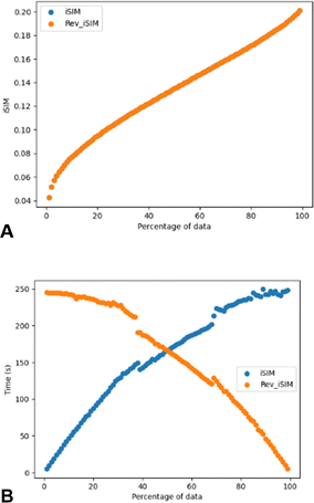
Another way of modifying the iSIM objective diversity metric that allows a faster diversity selection is what we called iSIMRevDiv: iSIM reversed diversity selection. In this algorithm we start with all the points, and we iterate to find the molecule that, if removed, would cause the remaining set to result in the lowest similarity value. This process is then repeated until the number of desired molecules is reached. iSIMRevDiv will be extremely useful in cases where more than 50% of the set wants to be picked. Fig. 7 show the iSIM and computing time comparison between the iSIMDiv and iSIMRev methods for the CHEMBL214 database represented by RDKIT fingerprints and using the iRR metric. Fig. 7A shows how when the diversity selection is started from the outlier, both forward and reversed iSIM diversity selection methods will yield the same average pairwise similarity results, which enables the user to use any of the two methods depending on the data percentage that wants to be picked. Fig. 7B shows computing times, and further supports the idea that for selections over 50% of the data the iSIMDivRev will be less computationally costly with the same high-quality results.
To further analyse the comparison of the iSIM diversity selection for both forward and reversed methods, random fingerprint datasets were generated, and the results were consistent with the ones previously observed (see Fig. S6†). The fact that diversity selection can be done in a reversed way makes iSIM diversity selection more attractive than typical algorithms like MaxMin where the computation of a pairwise similarity is required.
Up to this point, we have discussed algorithms that maximize the diversity (minimize the similarity) of the selected molecules. However, if the goal is to pick a diverse set and to also cover the underlying chemical space, these presented methods are not the best approach. Algorithms like MaxMin and the iSIM diversity selection maximize the diversity by picking the periphery of the chemical space (molecules that are the least similar to the rest), at the expense of completely overlooking other sections of chemical space, resulting in a low coverage.60
Using the complementary similarity, we can explore the chemical space with various approaches. Here, we propose five such methods. Fig. 8 shows graphically the explanation of each method. The first step for all the methods is to rank the molecules by increasing complementary similarity (as done in Fig. 5). After that, P molecules are selected based on the sector of the chemical space that wants to be sampled.
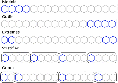 | ||
| Fig. 8 Graphical explanation of the medoid, outlier, extreme, stratified and quota sampling methods. | ||
- Medoid sampling: the P with the lowest complementary similarity.
- Outlier sampling: the P with the highest complementary similarity.
- Extremes sampling: the P/2 with the lowest complementary similarity and the P/2 with the highest complementary similarity.
- Stratified sampling: molecules are separated into b strata of the same size, then molecules with the lowest complementary in each stratum are picked until P is chosen. The default number of strata is the same as the number of molecules to pick, hence one molecule per stratum is picked. If an equal number of molecules per stratum are needed, the priority will be the strata with lower complementary similarity.
- Quota sampling: the range of complementary similarity (max–min) is separated into b strata of equal range. Molecules are assigned to a stratum based on their complementary similarity; each stratum will have the same complementary similarity range but not necessarily the same number of molecules. The default number of strata is ten. Molecules are picked from each stratum until P is reached; priority to molecules and strata with lower complementary similarity is given.
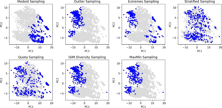
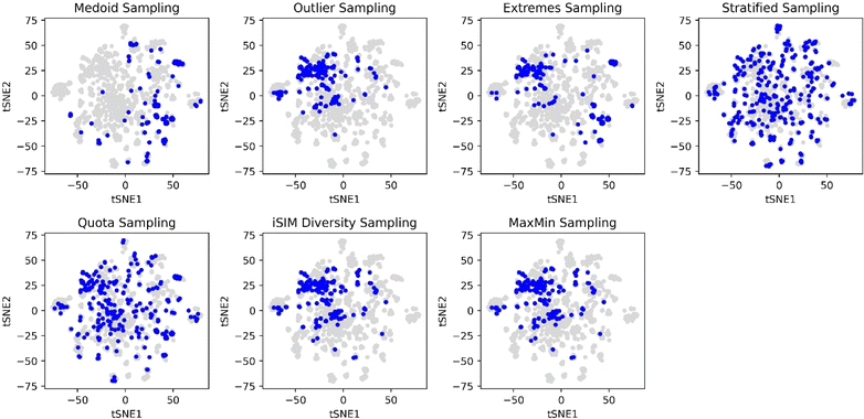
With the aim of comparing visually the selection methods proposed in this work, Principal Component Analysis (PCA)61,62 and t-Distributed Stochastic Neighbour Embedding (t-SNE)63 plots were generated and 10% of the ChEMBL214 selected by each method is identified. The iSIM Tanimoto complementary similarity was used to perform the initial sorting step. In Fig. 9 it can be seen how the medoid and outlier sampling methods pick the extremes of the set's chemical space. Intuitively, medoids have high values for the PC1 scores, and the outliers lower values. As expected, the extremes sampling is a mix between the medoids' and outliers' areas. It is relevant to point out that the iSIM diversity and MaxMin samplings pick molecules mostly from the same areas as the outlier sampling, proving the point that those algorithms maximize diversity but are not representative of the chemical space.
The selection methods that cover more of the chemical space are the stratified and quota samplings, with points spread through the two-dimensional space representation. Thus, if representativity is an important matter, we recommend these methods. Certain differences can be noticed between the two of them, the main one is that quota sampling includes more of the medoid and outlier regions than the stratified approach. The same trend in observations for the PCA was observed in the tSNE plots in Fig. 10.
Table 1 includes the iSIM (iT) values of the selected molecules by each method. Notice how the average similarities for the diversity and MaxMin methods are the lowest, which is the purpose of their algorithms. The outlier method has a closer similarity value to the MaxMin and diversity sampling, suggesting that they sample around the same area of the chemical space. The medoid sampling has the highest average similarity value, meaning that the molecules that are in the medoid area are highly similar. This could be an important tool to identify the “core” of a dataset. The values for extreme, stratified and quota are close to 0.33 which is the value for the whole set. For the quota and stratified methods this means that the selected molecules represent well the set, leading to an average similarity close to the complete set, supporting the visualization from previous figures. On the other hand, in the case of the extreme sampling this value is just a combination of two factors: low similarity values given by sampling from the extrema of the set compensated for by high similarity values whenever one is sampling within the outlier or the medoid region, resulting in a deceptively “average” iSIM value.
| Sampling method | iT |
|---|---|
| Medoid | 0.52405 |
| Outlier | 0.21217 |
| Extreme | 0.33403 |
| Stratified | 0.33066 |
| Quota | 0.32896 |
| iSIM diversity | 0.20132 |
| MaxMin | 0.20132 |
| Complete dataset | 0.33036 |
Clustering
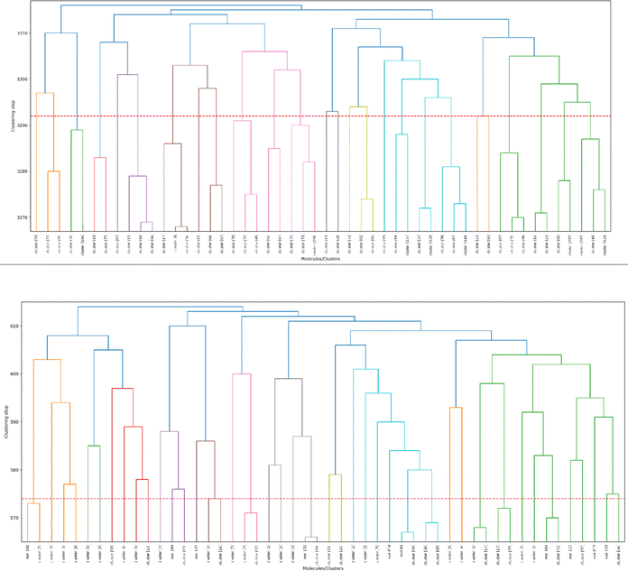
As a final proof-of-principle demonstration of the versatility of the iSIM framework, we look at the clustering of molecular libraries. While there are many ways in which the notion of comparing multiple elements at the same time could be applied to clustering problems, perhaps the most natural one is in the context of hierarchical agglomerative (HA) algorithms. Note that iSIM can be used as a linkage criterion in the sense that at any given point we can choose to combine the two sets that produce the largest iSIM value for their union. In more mathematical terms, given sets c1, c2, …, cK, we combine clusters i, j such that: i, j = argmaxp,qiSIM(cp∪cq). This is the criterion that we used in Fig. 11 to cluster the CHEMBL214 (N = 3317) and CHEMBL2835 (N = 615) libraries (using iSM and MACCS fingerprints). We can also use the computed iSIM values to determine the optimum number of clusters in the data. If we follow the evolution of iSIMk (the iSIM of the cluster formed in the kth step) we see that this quantity will tend to decrease with increasing k, but it will tend to reach some “stability” when an optimum separation of the data is achieved. In other words, we look for the largest value of k for which the quantity |iSIMk+1 − iSIMk| is as close to 0 as possible.Finally, clustering can be used to navigate through the molecular library, identifying representative structures associated with different basins in chemical space. For example, in Fig. 12 we show the medoids of the CHEMBL214 and CHEMBL2835 libraries in the case in which one selects 10 clusters in each of them. Note how our clustering is able to identify well-defined regions of chemical space that correspond to distinct scaffolds and functional groups. These structures, however, should not be mistaken for the most diverse structures in the original library. (A common practice in some fields tends to identify the cluster centroids with a diverse representation of the set.) For instance, if we calculate the iSIM for the set of medoids when one has a number of clusters equal to 10% of the total number of points, we get 0.766 and 0.810 for CHEMBL214 and CHEMBL2835, respectively, which is far from a maximally diverse set. That is, if the iSIMDiv and MaxMin tend to sample the data by increasing chemical diversity, the sampling through the medoids of the clusters offers a more “uniform” picture of the original set.
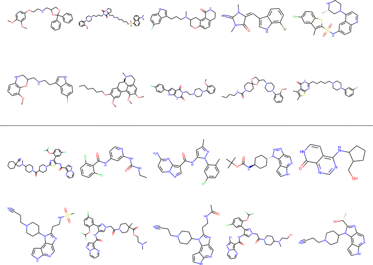 | ||
| Fig. 12 Medoids of each of the 10 colored clusters in the CHEMBL214 (top) and CHEMBL2835 (bottom) libraries using iSM on MACCS fingerprints. | ||
Conclusions
iSIM has the ability to perform the comparisons of multiple objects at the same time, irrespective of whether they are represented by binary fingerprints or real-value descriptors. The analytical mathematical operations behind iSIM and the evidence from randomly generated data and real molecule libraries show that the same exact value of average pairwise comparisons can be achieved for similarity indexes with the denominator equal to the length of the fingerprint, like RR and SM. In cases where the denominator is not equal to the length of the fingerprint, like T, iSIM still provides an exceptional approximation to the pairwise comparison average, highlighting the robustness of the mediant approximation theorem. This brings the two key advantages of iSIM: the much more attractive linear scaling O(N) compared to the traditional pairwise indices, and the greater simplicity (no need to define coincidence thresholds and weight functions) compared to our previous extended similarity indices.We showed that iSIM can be used to calculate the complementary similarity of each of the molecules in the library and a ranking can be done to identify and visualize molecules as part of high-density or low-density regions. Different diversity selection methods using the proposed framework can be applied depending on the necessity. iSIMDiv and iSIMRevDiv methods were developed to have two alternatives that output the same diversity results but differ in computing times depending on the percentage of data to select, adapting to the user's necessities. The iSIM metric can also be modified depending on whether the diversity selection is wanted to be globally or locally coerced, which can be done taking the square root of the iSIM counters to select data that will have a lower maximum pairwise similarity. Remarkably, all the proposed diversity selection methods have the same or better quality than the commonly used MaxMin. Another application of our work is hierarchical clustering, as we can use iSIM as a clustering objective function to be maximized when combining two molecules/clusters. The change in iSIM for the new cluster per clustering step can also be used as a metric to determine the optimal number of clusters. Overall, iSIM provides a flexible and easy-to-use framework to analyse molecular libraries, but that could be easily adapted to any problems that use comparisons between objects (metabolomics, MD simulations, etc.).
Finally, we want to discuss the computational gains offered by iSIM. That is, having shown the excellent agreement between the iSIM and the pairwise comparisons, the remaining question is: how much does the new O(N) algorithm help speed-up the comparison of large sets of molecules? For instance, the ChEMBL team reported that FPSim2 took ∼12 hours to compare the 1![[thin space (1/6-em)]](https://www.rsc.org/images/entities/char_2009.gif) 941
941![[thin space (1/6-em)]](https://www.rsc.org/images/entities/char_2009.gif) 405 compounds in ChEMBL 27 using a single core in an i9 laptop (https://chembl.github.io/FPSim2/source/user_guide/sim_matrix.html). On the other hand, Eloy Félix made public an independent test on the 2
405 compounds in ChEMBL 27 using a single core in an i9 laptop (https://chembl.github.io/FPSim2/source/user_guide/sim_matrix.html). On the other hand, Eloy Félix made public an independent test on the 2![[thin space (1/6-em)]](https://www.rsc.org/images/entities/char_2009.gif) 372
372![[thin space (1/6-em)]](https://www.rsc.org/images/entities/char_2009.gif) 674 molecules in ChEMBL 33 set using iSIM, which took less than 4 seconds to complete the same task (https://github.com/eloyfelix/iSIM/blob/main/isim_avg_set_sim.ipynb). That is, even the (poorly optimized) code accompanying this manuscript is capable of vastly outperforming (highly optimized) implementations based on pairwise comparisons when it comes to quantifying the chemical diversity of large datasets.
674 molecules in ChEMBL 33 set using iSIM, which took less than 4 seconds to complete the same task (https://github.com/eloyfelix/iSIM/blob/main/isim_avg_set_sim.ipynb). That is, even the (poorly optimized) code accompanying this manuscript is capable of vastly outperforming (highly optimized) implementations based on pairwise comparisons when it comes to quantifying the chemical diversity of large datasets.
Data availability
The software used to calculate the instant similarity indices, and all the other studies presented in the manuscript, can be found in https://github.com/mqcomplab/iSIM.Author contributions
KLP: conceptualization, data curation, investigation, methodology, software, validation, visualization, writing – original draft, writing – review & editing. TDK: conceptualization, investigation, methodology. RAMQ: conceptualization, investigation, methodology, funding acquisition, software, resources, supervision, writing – original draft, writing – review & editing.Conflicts of interest
There are no conflicts to declare.Acknowledgements
Research reported in this publication was supported by the National Institute of General Medical Sciences of the National Institutes of Health under award number R35GM150620. We thank Eloy Félix for his help with the ChEMBL timing benchmark, and Patrick Walters for his insightful remarks.References
- E. Fernández-de Gortari, C. R. García-Jacas, K. Martinez-Mayorga and J. L. Medina-Franco, J. Cheminf., 2017, 9, 9 Search PubMed.
- R. Todeschini and V. Consonni, Handbook of Molecular Descriptors, Wiley, 2000 Search PubMed.
- S. Gugler and M. Reiher, J. Chem. Theory Comput., 2022, 18, 6670–6689 CrossRef CAS PubMed.
- P. Jaccard, New Phytol., 1912, 11, 37–50 CrossRef.
- D. J. Rogers and T. T. Tanimoto, Science, 1960, 132, 1115–1118 CrossRef CAS PubMed.
- R. Todeschini, V. Consonni, H. Xiang, J. Holliday, M. Buscema and P. Willett, J. Chem. Inf. Model., 2012, 52, 2884–2901 CrossRef CAS PubMed.
- M. A. Johnson, G. M. Maggiora, et al., Concepts and applications of molecular similarity, Wiley-Interscience, 1st edn, 1990 Search PubMed.
- G. Hu, G. Kuang, W. Xiao, W. Li, G. Liu and Y. Tang, J. Chem. Inf. Model., 2012, 52, 1103–1113 CrossRef CAS PubMed.
- V. Zoete, A. Daina, C. Bovigny and O. Michielin, J. Chem. Inf. Model., 2016, 56, 1399–1404 CrossRef CAS PubMed.
- H. Eckert and J. Bajorath, Drug Discovery Today, 2007, 12, 225–233 CrossRef CAS PubMed.
- J. M. Cohen, J. W. Rice and T. A. Lewandowski, ACS Sustain. Chem. Eng., 2018, 6, 1941–1950 CrossRef CAS.
- B. A. Posner, H. Xi and J. E. J. Mills, J. Chem. Inf. Model., 2009, 49, 2202–2210 CrossRef CAS PubMed.
- X. Ning, H. Rangwala and G. Karypis, J. Chem. Inf. Model., 2009, 49, 2444–2456 CrossRef CAS PubMed.
- E. A. Helgee, L. Carlsson, S. Boyer and U. Norinder, J. Chem. Inf. Model., 2010, 50, 677–689 CrossRef CAS PubMed.
- W. P. van Hoorn and A. S. Bell, J. Chem. Inf. Model., 2009, 49, 2211–2220 CrossRef CAS PubMed.
- R. Buonfiglio, O. Engkvist, P. Várkonyi, A. Henz, E. Vikeved, A. Backlund and T. Kogej, J. Chem. Inf. Model., 2015, 55, 2375–2390 CrossRef CAS PubMed.
- D. Stumpfe and J. Bajorath, J. Med. Chem., 2012, 55, 2932–2942 CrossRef CAS PubMed.
- M. P. Krein and N. Sukumar, J. Phys. Chem. A, 2011, 115, 12905–12918 CrossRef CAS PubMed.
- D. J. Huggins, A. R. Venkitaraman and D. R. Spring, ACS Chem. Biol., 2011, 6, 208–217 CrossRef CAS PubMed.
- G. M. Downs, P. Willett and W. Fisanick, J. Chem. Inf. Comput. Sci., 1994, 34, 1094–1102 CrossRef CAS.
- P. Kovács, F. Tran, A. Hanbury and G. K. H. Madsen, J. Chem. Theory Comput., 2022, 18, 441–447 CrossRef PubMed.
- G. Maggiora, M. Vogt, D. Stumpfe and J. Bajorath, J. Med. Chem., 2013, 57, 3186–3204 CrossRef PubMed.
- G.-L. Xiong, Y. Zhao, L. Liu, Z.-Y. Ma, A.-P. Lu, Y. Cheng, T.-J. Hou and D.-S. Cao, J. Med. Chem., 2021, 64, 7544–7554 CrossRef CAS PubMed.
- B. Zhang, M. Vogt, G. M. Maggiora and J. Bajorath, J. Comput.-Aided Mol. Des., 2015, 29, 595–608 CrossRef CAS PubMed.
- D. Lemm, G. Falk von Rudorff and O. Anatole von Lilienfeld, Machine Learning: Science and Technology, 2023, 4, 045043 Search PubMed.
- H. Ding, I. Takigawa, H. Mamitsuka and S. Zhu, Briefings Bioinf., 2014, 15, 734–747 CrossRef PubMed.
- H. Safizadeh, S. W. Simpkins, J. Nelson, S. C. Li, J. S. Piotrowski, M. Yoshimura, Y. Yashiroda, H. Hirano, H. Osada, M. Yoshida, C. Boone and C. L. Myers, J. Chem. Inf. Model., 2021, 61, 4156–4172 CrossRef CAS PubMed.
- J. L. Bentley, Commun. ACM, 1975, 18, 509–517 CrossRef.
- J. H. Friedman, J. L. Bentley and R. A. Finkel, ACM Transactions on Mathematical Software, 1977, 3, 209–226 CrossRef.
- S. M. Omohundro, Five Balltree Construction Algorithms, International Computer Science Institute, 1989, pp. 1–22 Search PubMed.
- E. Felix, chembl/FPSim2: simple package for fast molecular similarity searches, https://github.com/chembl/FPSim2, accessed 4 February 2024 Search PubMed.
- A. Dalke, J. Cheminf., 2019, 11, 1–21 Search PubMed.
- D. K. Agrafiotis and V. S. Lobanov, J. Chem. Inf. Comput. Sci., 1999, 39, 51–58 CrossRef CAS.
- D. B. Turner, S. M. Tyrrell and P. Willett, J. Chem. Inf. Comput. Sci., 1997, 37, 18–22 CrossRef CAS.
- J. D. Holliday, S. S. Ranade and P. Willett, Quant. Struct.-Act. Relat., 1995, 14, 501–506 CrossRef CAS.
- R. A. Miranda-Quintana, D. Bajusz, A. Rácz and K. Héberger, J. Cheminf., 2021, 13, 32 Search PubMed.
- R. A. Miranda-Quintana, A. Rácz, D. Bajusz and K. Héberger, J. Cheminf., 2021, 13, 33 Search PubMed.
- J. Verhellen, Chem. Sci., 2022, 13, 7526–7535 RSC.
- L. Chang, A. Perez and R. A. Miranda-Quintana, Phys. Chem. Chem. Phys., 2022, 24, 444–451 RSC.
- A. Rácz, L. M. Mihalovits, D. Bajusz, K. Héberger and R. A. Miranda-Quintana, J. Chem. Inf. Model., 2022, 62, 3415–3425 CrossRef PubMed.
- T. B. Dunn, G. M. Seabra, T. D. Kim, K. E. Juárez-Mercado, C. Li, J. L. Medina-Franco and R. A. Miranda-Quintana, J. Chem. Inf. Model., 2022, 62, 2186–2201 CrossRef CAS PubMed.
- R. Pikalyova, Y. Zabolotna, D. Horvath, G. Marcou and A. Varnek, J. Chem. Inf. Model., 2023, 63, 4042–4055 CrossRef CAS PubMed.
- E. A. Flores-Padilla, K. E. Juárez-Mercado, J. J. Naveja, T. D. Kim, R. Alain Miranda-Quintana and J. L. Medina-Franco, Mol. Inf., 2022, 41, 2100285 CrossRef CAS PubMed.
- T. B. Dunn, E. López-López, T. D. Kim, J. L. Medina-Franco and R. A. Miranda-Quintana, Mol. Inf., 2023, 42, 2300056 CrossRef CAS PubMed.
- A. Rácz, T. B. Dunn, D. Bajusz, T. D. Kim, R. A. Miranda-Quintana and K. Héberger, J. Comput.-Aided Mol. Des., 2022, 36, 157–173 CrossRef PubMed.
- I. Redžepović and B. Furtula, Mol. Diversity, 2023, 27, 1603–1612 CrossRef PubMed.
- K. López-Pérez, E. López-López, J. L. Medina-Franco and R. A. Miranda-Quintana, Molecules, 2023, 28, 6333 CrossRef PubMed.
- P. F. Russell and T. R. Rao, et al. , J. Malar. Inst. India, 1940, 3, 153–178 Search PubMed.
- R. R. Sokal and C. D. Michener, University of Kansas science bulletin, University of Kansas, 1958 Search PubMed.
- S. B. Guthery, A motif of mathematics, Docent Press, 2011 Search PubMed.
- E. R. Tou, Math Horizons, 2017, 24, 8–11 CrossRef.
- C. R. Harris, K. J. Millman, S. J. van der Walt, R. Gommers, P. Virtanen, D. Cournapeau, E. Wieser, J. Taylor, S. Berg, N. J. Smith, R. Kern, M. Picus, S. Hoyer, M. H. van Kerkwijk, M. Brett, A. Haldane, J. F. del Río, M. Wiebe, P. Peterson, P. Gérard-Marchant, K. Sheppard, T. Reddy, W. Weckesser, H. Abbasi, C. Gohlke and T. E. Oliphant, Nature, 2020, 585, 357–362 CrossRef CAS.
- Random—generate pseudo-random numbers—Python 3.12.3 documentation, https://docs.python.org/3/library/random.html, accessed 17 April 2024.
- D. van Tilborg, A. Alenicheva and F. Grisoni, J. Chem. Inf. Model., 2022, 62, 5938–5951 CrossRef CAS PubMed.
- RDKit, RDKit: open-source cheminformatics, https://www.rdkit.org Search PubMed.
- J. L. Durant, B. A. Leland, D. R. Henry and J. G. Nourse, J. Chem. Inf. Comput. Sci., 2002, 42, 1273–1280 CrossRef CAS PubMed.
- H. L. Morgan, J. Chem. Doc., 1965, 5, 107–113 CrossRef CAS.
- F. Parreño, R. Álvarez-Valdés and R. Martí, European Journal of Operational Research, 2021, 289, 515–532 CrossRef.
- C. Kuo, F. Glover and K. S. Dhir, Decision Sciences, 1993, 24, 1171–1185 CrossRef.
- D. J. Woodward, A. R. Bradley and W. P. Van Hoorn, J. Chem. Inf. Model., 2022, 2022, 4402 Search PubMed.
- R. Bro and A. K. Smilde, Anal. Methods, 2014, 6, 2812–2831 RSC.
- G. Ivosev, L. Burton and R. Bonner, Anal. Chem., 2008, 80, 4933–4944 CrossRef CAS PubMed.
- L. der Maaten and G. Hinton, Journal of Machine Learning Research, 2008, 2579–2605 Search PubMed.
Footnote |
| † Electronic supplementary information (ESI) available. See DOI: https://doi.org/10.1039/d4dd00041b |
| This journal is © The Royal Society of Chemistry 2024 |


