
Optical single molecule characterisation of natural and synthetic polymers through nanopores†
Charlotte
de Blois
 ab,
Marie
Engel
b,
Marie-Amélie
Rejou
b,
Bastien
Molcrette
a,
Arnaud
Favier
*b and
Fabien
Montel
*a
ab,
Marie
Engel
b,
Marie-Amélie
Rejou
b,
Bastien
Molcrette
a,
Arnaud
Favier
*b and
Fabien
Montel
*a
aUniv. Lyon, ENS de Lyon, CNRS, Laboratoire de Physique, F-69342 Lyon, France. E-mail: fabien.montel@ens-lyon.fr
bUniversité de Lyon, CNRS, Université Claude Bernard Lyon 1, INSA Lyon, Université Jean Monnet, UMR 5233, Ingénierie des Matériaux Polymères, F-69621 Villeurbanne, France. E-mail: arnaud.favier@univ-lyon1.fr
First published on 20th November 2023
Abstract
Nanopore techniques are now widely used to sequence DNA, RNA and even oligopeptide molecules at the base pair level by measuring the ionic current. In order to build a more versatile characterisation system, optical methods for the detection of a single molecule translocating through a nanopore have been developed, achieving very promising results. In this work, we developed a series of tools to interpret the optical signals in terms of the physical behaviour of various types of natural and synthetic polymers, with high throughput. We show that the measurement of the characteristic time of a translocation event gives access to the apparent molecular weight of an object, and allows us to quantify the concentration ratio of two DNA samples of different molecular weights in solution. Using the same tools for smaller synthetic polymers, we were able to obtain information about their molecular weight distribution depending on the synthesis method.
Introduction
Synthesis and characterisation of natural polymers at the monomer level are routinely performed in living cells by a broad range of biological enzymes like DNA and RNA polymerases and ribosome and glycosyltransferases. The same characterisation remains a challenge for synthetic polymers, but several promising approaches based on single molecule manipulation and characterisation techniques have been used in the past few years. Atomic force microscopy offers the ability to manipulate single polymers and access their mechanical response at the single-molecule level. It is now commonly used to characterise DNA (single-stranded and double-stranded), RNA and protein structures and their mechanics.1 It can also be used to determine the Kuhn length and segment elasticity of various synthetic polymers such as polystyrene, poly(vinyl alcohol), poly(N-vinyl-2-pyrrolidone) and even carboxymethylcellulose. Mainly used to analyse natural polymers, optical tweezers2 have also been used to characterise the mechanics of synthetic polymers such as poly(methyl methacrylate) in different solvents. Nanopore techniques are now widely used to sequence DNAs, RNAs3,4 and even oligopeptide molecules at the base pair level.5 They have been shown to efficiently characterise the molecular weight distribution of PEG molecules,6 or simultaneously detect translocations of individual free fluorophores of different colours.7 Complex microfluidic devices have also been developed,8 for instance for the direct observation of the translocation of ultra-long (>200 MDa) DNA molecules. Finally, the first recordings of the interaction between a synthetic homopolymer and biological nanopores9 showed promising results in capturing some of the polymer properties, such as the flexibility of the polymer, and also highlighted the difficulty of directly reading a polymer translocating through nanopores.Despite these results and their high sensitivity, these approaches are limited by the adaptability to the studied polymer and/or the rate of measurements. In order to build a versatile and high throughput tool that can be used on various types of natural and synthetic polymers we propose a method based on the optical detection10,11 of single polymer molecules through nanopores. It has been shown12 for instance that the translocation time of DNA molecules through nanopores depends on the molecule's conformation at the beginning of the translocation process, with extended molecules having a longer translocation time.
In this work, we have modified and extended the zero mode waveguide for nanopores previously developed in our group13 to achieve high frequency and high throughput detection and characterisation of natural and synthetic polymers by the same device. Compared to electrical detection, optical sensors coupled with nanopores enable the direct visualisation of successful translocation events and are more efficient in dealing with a high number of pores in parallel. They also give more ease in the choice of the translocated object (DNA, polymers, proteins, viruses, etc.) without adapting the detection device.7,11,14–17
In a prior study, we showed that the hydrodynamic propulsion of DNA molecules was limited by a critical pressure, and we examined the translocation frequency and the total duration of translocation events as a function of pore size and pressure.13 The event detection was done manually and was restricted in terms of the number of simultaneous events and the temporal resolution of the entire events, limiting the possibility of systematically characterising the events. In this work, we developed a novel approach based on automated image analysis to characterise the entire fluorescence signal of an object passing through nanopores and to extract physical information for both natural and synthetic polymers. This approach enabled a finer analysis of the temporal process of an event as we defined two characteristic times, the exit time and the ejection time (Fig. 1).
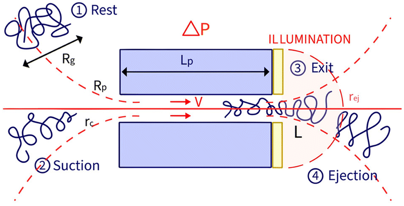 | ||
| Fig. 1 Illustration of the translocation of a polymer through a nanopore, and introduction of the notations. (1) At rest, the polymer takes a statistical coil conformation with a radius of gyration Rg. (2) When driven by the flow, above a critical shear rate the polymer is deformed, following the affine deformation model. If its transverse deformation is smaller than the pore radius, the polymer may enter the nanopore. (3) The polymer exits the nanopore on the golden-coated side of the membrane. The zero-mode waveguide illumination excites the fluorophore from the membrane exit but does not reach inside of the pore. Only the part of the polymer that has exited the nanopore gives a signal. (4) After exiting the nanopore, the polymer is ejected away from the membrane by the flow field and eventually leaves the illumination plane. | ||
Our experimental setup and image analysis tools were initially validated using the reference λ DNA molecule. We then investigated DNA molecules with different molecular weights. The characteristic event times were compared with theoretical values computed using the classical polymer theory of de Gennes and the suction model. Subsequently, by studying the distribution of event characteristics in a solution containing two DNAs of different molecular weights, we demonstrated that quantitative information can be accessed about the concentration ratio of the two DNA samples. Finally, our method was applied to the study of smaller synthetic polymers. We synthesised the same polymer using two different methods, one yielding low dispersity and the other high dispersity in the distribution of the molecular weights. Although limitations in the current optical system might lead to the overlooking of translocation events involving low molecular weight molecules, we still robustly identified a difference in the dispersity of event intensity between the two polymer samples.
Materials and methods
We studied the pressure-driven translocation of different polymers, bio-polymers (double-stranded DNA of various molecular weights) and synthetic polymers, through membranes presenting nanopores with a controlled nominal radius Rp = 25, 50 or 100 nm. The fluorescently labelled polymer molecules were optically detected at the exit of the nanopores using a zero-mode waveguide illumination.18DNA samples
Double-stranded DNAs of different molecular weights were used (some characteristics are summarised in Table 1):• T4 DNA: T4GT7 DNA (no. 74001F Nippon Gene), linear
• λ DNA: λ-phage DNA (#SD0011 Thermo Scientific), linear
• ΦX DNA: ΦX174RFII DNA (N3022L Biolabs), linear
• pNEB DNA: pNEB206A DNA (#N55025 Biolabs), linear
DNA was labelled with the Yoyo-1 dye (Life Technologies), at a ratio of 1 μL of Yoyo to 1 μg of DNA.13 DNA solutions were prepared in Tris and EDTA buffer (TE buffer, pH 7.4) at 10 fM, except for ΦX DNA which was prepared at 100 fM to obtain a statistically significant number of events.
| DNA | N bp | M w (MDa) | R g (nm) | Pe | L* (μm) |
|---|---|---|---|---|---|
The radius of gyration is computed using the worm-like chain model,  , with , with ![[small script l]](https://www.rsc.org/images/entities/i_char_e146.gif) p = 48 nm, the persistence length of DNA, c = Nbpa the contour length of a DNA molecule, and a = 0.34 nm, the size of a DNA base pair. The Peclet number Pe (eqn (26)) and the total length of a DNA molecule at the exit of the nanopore L* (eqn (S5) and (S9) in the ESI S2†) are given for the experiments conducted in nanopores of radius Rp = 45 nm, under a flow driven by a pressure gradient ranging from ΔP = 10 to 100 mbar. L* is to be compared with the total thickness of the illumination region, 0.76 μm. p = 48 nm, the persistence length of DNA, c = Nbpa the contour length of a DNA molecule, and a = 0.34 nm, the size of a DNA base pair. The Peclet number Pe (eqn (26)) and the total length of a DNA molecule at the exit of the nanopore L* (eqn (S5) and (S9) in the ESI S2†) are given for the experiments conducted in nanopores of radius Rp = 45 nm, under a flow driven by a pressure gradient ranging from ΔP = 10 to 100 mbar. L* is to be compared with the total thickness of the illumination region, 0.76 μm. |
|||||
| T4 DNA | 163![[thin space (1/6-em)]](https://www.rsc.org/images/entities/char_2009.gif) 636 636 |
108 | 943 | 75–2100 | 2.7–3.3 |
| λ DNA | 48502 |
31.5 | 513 | 9.7–270 | 1.4–1.8 |
| ΦX DNA | 5386 | 3.5 | 169 | 0.32–6.9 | 0.45–0.56 |
| pNEB DNA | 2722 | 1.8 | 118 | 0.16–2.5 | 0.30–0.38 |
Synthetic polymers
Synthesis and characterisation of fluorescent polymer chains were based on a previously reported strategy.19 Briefly, the synthetic fluorescent polymers were prepared from poly(N-acryloylmorpholine-stat-N-acryloxysuccinimide), poly(NAM-stat-NAS), reactive copolymer precursors obtained by radical polymerisation. At the azeotropic composition (NAM/NAS 60/40 molar ratio) the reactive NAS units are regularly distributed along the polymer chains.20 The reactive poly(NAM-stat-NAS) skeleton was then functionalized in the lateral position of the chains by reacting the activated ester groups of the NAS units. The coupling of a controlled number of amino-derived fluorophores and PEG branches was followed by hydrolysis, leading to fully water-soluble polymers. The full structure of the polymer is given in the ESI, Fig. S1.†PolyHD. The high molecular weight poly(NAM-stat-NAS) copolymer was prepared by conventional radical polymerisation. NAM (338.8 mg, 2.4 mmol), NAS (270.6 mg, 1.6 mmol), 2,2′-azobis(isobutyronitrile) AIBN (0.82 mg, 4.98 × 10⁻⁶ mol) and trioxane were dissolved in dioxane (1.7 mL) in a Schlenk tube. The reaction mixture was de-oxygenated by three consecutive freeze–pump–thaw cycles and then heated at 80 °C for 1 h in a thermostated oil bath.
PolyLD. The high molecular weight poly(NAM-stat-NAS) copolymer was prepared by RAFT polymerisation. NAM (338.8 mg, 2.4 mmol), NAS (270.6 mg, 1.6 mmol), 2-[[(2-carboxyethyl)sulfanylthiocarbonyl]-sulfanyl]propanoic acid (CTTC, Sigma Aldrich, ≥95%, 0.31 mg, 1.2 × 10⁻⁶ mol), lithium phenyl-2,4,6-trimethylbenzoylphosphinate (LAP, Sigma Aldrich, ≥95%, 0.036 mg, 1.22 × 10⁻⁷ mol) and trioxane were dissolved in dioxane (1.7 mL) in a Schlenk tube. The reaction mixture was de-oxygenated by three consecutive freeze–pump–thaw cycles and then subjected for 5 min to 365 nm blue LED irradiation (HepatoChem photoreactor) at room temperature.
In both cases, monomer conversion was determined by 1H NMR using trioxane as the internal reference and absolute polymer molecular weight distributions were analysed by size exclusion chromatography coupled with multi-angle laser light scattering detection (SEC-MALLS). The copolymers were purified by two consecutive precipitations in diethyl ether and then dried under vacuum to a constant weight.
Size exclusion chromatography with online multi-angle laser light scattering detection (SEC-MALLS). SEC-MALLS was performed in chloroform with a mixed-C PL gel column (5 μm pore size) and a LC-6A Shimadzu pump (1 mL min−1). Online double detection was carried out using a differential refractometer (Waters DRI 410) and a MiniDAWN TREOS three-angle (46°, 90°, 133°) light scattering detector (Wyatt Technologies) operating at 658 nm. Analyses were run by injection of polymer solutions (3 g L−1, 70 μL). The specific refractive index increment (dn/dc) of poly(NAM-stat-NAS) in chloroform (0.130 mL g−1) was previously determined with an NFT-scan interferometer operating at 633 nm. The molecular weight distribution data were obtained using the Wyatt ASTRA SEC/LS software package. The full chromatogram and the full distribution of the molecular weight of both polymers are given in the ESI S3, Fig. S2 and S3.†
1H nuclear magnetic resonance (NMR). 1H NMR experiments were recorded using a Bruker AVANCE III spectrometer operating at 400.13 MHz.
Size exclusion chromatography with online UV/Vis detection (SEC-UV). Size exclusion chromatography coupled with UV/Vis detection was performed using a Waters 1515 isocratic HPLC pump (flow rate: 1 mL min−1) and a Styragel HR3 Waters column (7.8 × 300 mm2). The eluent was dimethylformamide (DMF) with LiBr (0.05 mol L−1) at 30 °C. Detection was carried out using both a Waters 2410 refractive index detector and a Waters 2489 UV-visible detector set at 488 nm. Data acquisition and treatment were performed using the Breeze software (Waters). The SEC-UV analysis of the fluorophore is given in the ESI, Fig. S4.†
Membranes and chambers
We used track-etched membranes (Whatman, with nominal pore radius Rnomp equal to 25, 50, or 100 nm and thicknesses Lp equal to 6, 6, and 10 μm, respectively), coated with a thin layer of gold (Plassys MEB 550 S evaporator, a thickness of 50 nm and a surface roughness of 2.5 nm). The membranes were illuminated from the (golden) cis-side by an extended laser beam. The gold layer induces a zero-mode waveguide illumination18 at the end of the pores. The radius of the nanopores after gold coating Rp was measured13 using scanning electron microscopy, as summarised in Table 2.| R nomp | R p | L p |
|---|---|---|
| The nominal pore radius Rnomp and the length of the pores are provided by the manufacturer. The pore radius after gold deposition was characterised through scanning electron microscopy, with detailed measurements available in previous works.13,15 | ||
| 25 nm | 21 nm | 6 μm |
| 50 nm | 45 nm | 6 μm |
| 100 nm | 110 nm | 10 μm |
The gold-coated membrane was stored under dry conditions. Before the experiment, the membrane was soaked for 10 min in a 0.1 M solution of HCl, for cleaning, and then rinsed with Milli-Q water (Millipore). The membrane was then used immediately.
The chamber design is presented in Fig. 2. The upper chamber (i) is obtained by piercing a 3 mm hole in a 1 cm cap. The cap can be screwed to the pressure tubing (ii). The membrane (iii) is directly attached to the cap using a single layer of double-sided tape. A second single layer of tape is placed on top of the membrane. The lower chamber (iv) is 3D printed, circular with a 2 cm radius and a glass bottom slide (v). The upper chamber is placed inside the lower chamber using three plots (vi) of controlled height (two layers of double-sided tape 100 μm). The upper chamber is filled with the polymer solution and the lower chamber with the buffer solution (TE for DNA solutions and PBS for polymer solutions).
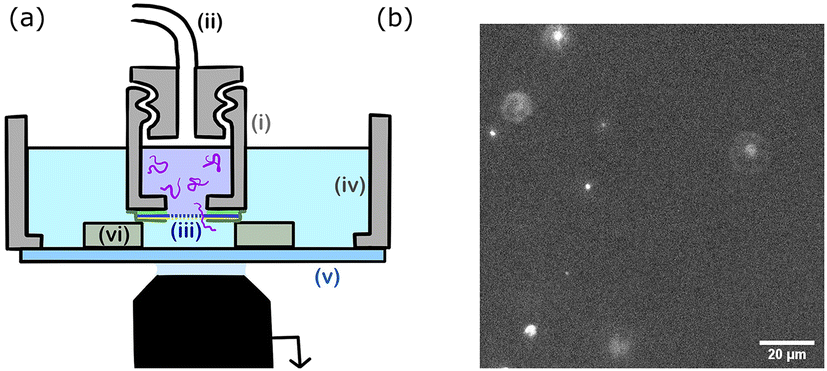 | ||
| Fig. 2 (a) Illustration of the experimental set-up. The upper chamber (i), a cap with a 3 mm hole at the bottom is filled with the polymer solution, and screwed to the pressure tubing (ii). The gold-coated nanopore membrane (iii) is placed over the cap's hole. The cap is placed in the chamber (iv) and separated from the bottom glass slide (v) by three spacers (vi). The chamber is filled with the buffer solution and placed on the microscope objective to perform the imaging through the bottom glass slide. (b) Acquired image of the translocation of λ DNA molecules through a Rp = 45 nm nanopore membrane at ΔP = 50 mbar. Several translocation events (bright spots) are observed simultaneously. Unlike the images used for data analysis, this image was acquired with no binning, at a frequency of 33 Hz. | ||
Before the experiments with the synthetic polymers, the gold layer was passivated using a fresh PBS solution containing 10 μM tris(2-carboxyethyl)phosphine hydrochloride, TCEP (Thermo Scientific Pierce) and 10 μM thiol-terminated poly(N-acryloylmorpholine) polymer (PNAM-SH, 10 kDa, Đ = 1.1, synthesised as previously described).21,22
Nanopore experiments
The whole device was placed on an inverted fluorescence microscope (Zeiss Axiovert 200). Observations were made through the glass bottom slide, with a focus on the membrane. All experiments are conducted at room temperature (25 °C).The transport of the fluorescent single molecules through the nanopores was observed using a laser source (Cobalt Blues), an electron multiplying charge-coupled device camera (Andor, iXon 897), and a 60× water objective (an observation field of 125 × 125 μm2). A polymer molecule inside a pore is invisible until it reaches the volume illuminated by the evanescent field. The fluorescence eventually disappears because of optical defocusing as the molecules are advected away from the membrane. We used a pressure microcontroller (MFCS, Fluigent, Paris) with a pressure resolution better than 0.1 mbar. A set of experiments was conducted using the same membrane by increasing the pressure step by step from 0 mbar (no event), to a maximum pressure that depended on the pore radius, then decreasing the pressure back to 0 mbar, to check for the absence of hysteresis that may be caused by the clogging of the nanopores. At each step, after waiting for pressure stabilisation (typically a few tens of seconds), the experiment was recorded at constant pressure.
Images were acquired at a frequency of 176 Hz, using a camera binning of 8 to maximise the intensity of an event. The gain was 30 for the DNA and 300 for the synthetic polymers as the former exhibited a higher fluorescence intensity.
A typical experiment consisted in recording 4000 images of 512 × 512 pixels, during 22.7 seconds, observing a few hundred translocation events. An example of 10 s of image acquisition is given in the ESI (Movie S1†), with no binning and an acquisition frequency of 33 Hz. The upper chamber was filled with a solution of λ DNA prepared as mentioned previously, and a pressure gradient of ΔP = 50 mbar was applied across the membrane of nanopores Rp = 45 nm. Each bright spot is a translocation event.
Image processing and analysis
We defined an event as the translocation of one polymer chain through a nanopore. We developed a homemade Matlab® code to accurately detect and process a large number of simultaneous events. The segmentation of all events is computed in three major steps:(1) Image processing: A background image is first computed from the time average of all raw images, and subtracted. To improve the signal-to-noise ratio and facilitate the detection of events, a light temporal filter (continuous averaging over six images) is applied to the images.
(2) Event segmentation: An intensity threshold is determined manually for one set of experiments (same membrane, different pressures), by comparing the intensity of many pixels in the absence of an event (0 mbar experiments) with the intensity of many pixels with some events (high-pressure experiments). The 3D stack of images is segmented, and all connected voxels are associated with one unique event, using the bwconn3 function of Matlab®. The intensity of the event is then computed from the raw images by summing the intensity of all participating pixels, at all times.
(3) Event selection: Selection criteria are applied to discriminate ‘good’ events. The ‘bad’ events we removed are typically two events not resolved in time, events out of the focus region on the membrane and aberrant events consisting of only one very intense voxel.
A typical series of events over a few seconds for the translocation of λ DNA through the Rp = 45 nm nanopore at ΔP = 50 mbar is given Fig. 3(a).
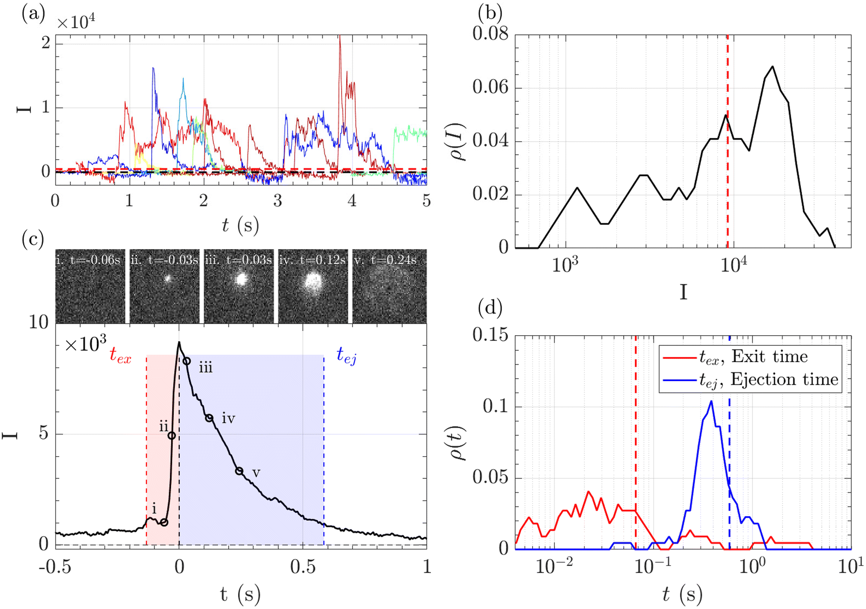 | ||
| Fig. 3 Illustration of the data analysis process for the translocation of λ DNA through a membrane of Rp = 45 nm nanopores, at ΔP = 50 mbar. (a) Evolution of the intensity with time of some pixels presenting large intensity fluctuation corresponding to the passage of a polymer. The horizontal red dashed line represents the segmentation threshold. (b) Density of probability of the maximum intensity of each event. The vertical red dashed line shows the maximum intensity of the mean event. (c) Mean event computed by averaging all segmented events. The exit time, in red, corresponds to the time taken by the polymer to exit a nanopore. The ejection time, in blue, corresponds to the time taken by the polymer to move outside the illumination region. Images of a typical event are shown: (i) before the event, (ii) apparition of the event, (iii) the event is growing in width and intensity until it reaches a maximum, (iv) the event starts exiting the illumination region, (v) the intensity decreases until the event completely leaves the illumination region. (d) Density of probability of the exit times (in red) and ejection times (in blue) measured for each event. The vertical dashed lines correspond to the respective times measured on the mean event. | ||
The zero-mode waveguide illumination strongly depends on the local geometry of the membrane and may vary locally as the nanopores are randomly distributed. On the other hand, when exiting a nanopore, a polymer is driven by the extensional flow and may follow any streamline, from one that is perpendicular to the nanopore to the one close to the membrane. Because of these effects and thermal fluctuations, a very large variety of events were observed with different maximum intensities, shapes and times. As such, events cannot be compared individually, and statistical tools are required for analysis. We thus proposed a series of such tools and used them in a typical experiment with λ DNA through the Rp = 45 nm nanopore at ΔP = 50 mbar (Fig. 3). The maximum intensity of every event was first computed. Then, the time at which an event reached half of its maximum was used to centre all events in time and their mean intensity was computed (Fig. 3(b)). The mean event was composed of a fast-rising time (red region) and a slow exponentially decreasing time (blue region). The same observation was made on each individual event. By comparing the evolution of the intensity vs. time with the live observation of an event on the camera, we noticed that the rising time corresponded to the apparition and growth of a focused spot (images (i) to (ii)), while the decreasing time corresponded to the defocalisation of the spot (images (iii) to (v)). As such we identified the first time as the ‘exit’ time tex, a time when the polymer is leaving the nanopore while still being partially inside, and the second time as the ‘ejection’ time tej, a time when the polymer has completely left the nanopore and is advected away by the flow.
To measure these times accurately, two separate fitting procedures were defined for the two parts of the curves on both sides of their maximum. The exit time was fitted using a sigmoid function with four parameters:
| I = a + b/(1 + exp(−(x − c)/d)). | (1) |
ln(81).
The ejection time was fitted using a decaying exponential with four parameters
| I = a′ + b′e(c′−x)/d′. | (2) |
ln(10).
The maximum intensities, exit times and ejection times of all events were used to investigate the statistical properties of the object. Typically, the densities of probability were computed, Fig. 3(c) and (d). Direct measurement gave very dispersed values. The maximum intensity, the exit time and the ejection time were thus measured from the mean intensity of all events, as represented in the Fig. 3(c) by vertical lines. This method was found to be less sensitive to aberrant events than the direct measure.
DNA transport
Modelling the transport of DNA
In this section, we introduce the models used to describe the translocation of DNA and identify the relevant physical quantities to be considered experimentally. Polymers, and in particular DNA molecules must stretch when confined in nanochannels smaller than their size.23–26 This stretching is governed by self-avoidance interactions, and different translocation regimes have been identified depending on the confinement of the molecule. Under the experimental conditions explored in this paper, the molecules inside the nanopore are in the de Gennes regime or extended de Gennes regime. We are interested in the behaviour of the molecules at the exit of the nanopore when the molecule is deformed and advected by an extensional flow. Under these conditions, we always considered them to be in the de Gennes regime, meaning that the stretched molecule can be seen as a succession of blobs of radius determined by the local hydrodynamic shear stresses. Then as the polymer is advected further away from the membrane, it eventually reaches its bulk configuration, a statistical coil of size Rg.Let us consider a nanopore of radius Rp and length Lp separating two regions filled with a fluid of viscosity η. The geometry is illustrated in Fig. 1. Across the nanopore, a hydrostatic pressure gradient ΔP is applied. A constant flow Q is established through the nanopore,
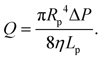 | (3) |
On one side, a polymer is dragged by the flow toward the membrane. At the entrance and at the exit of the nanopore, we suppose that the flux is extensional and that the polymer only feels the shear rate σ exerted by the solvent:
 | (4) |
 | (5) |
| ξ(σ < σZ) = Rg | (6) |
 | (7) |
We also define the distance from the nanopore rZ at which the shear rate and the Zimm critical stress become equal, and the polymer starts deforming:
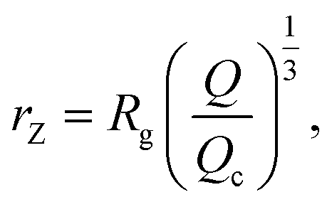 | (8) |
| rZ < Rg, | (9) |
 | (10) |
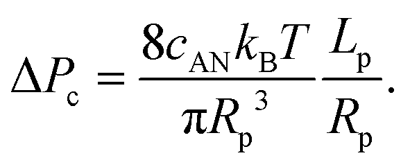
Interestingly, the critical pressure only depends on the geometry of the nanopore and not on the polymer molecular weight, which is confirmed by the experimental observations13 of the translocation of λ DNA through nanopores of different radii and lengths.
 | (11) |
 | (12) |
The blob radius depends on the shear stress imposed by the flow, which decreases as the polymer gets further away from the nanopore. The polymer that has left the nanopore takes a trumpet shape, with its constitutive blobs getting larger downstream from the pore.
For computing the exit time, we consider only the succession of Nb blobs at the nanopore, of radius ξ(Rp). By conservation of the total number of monomers, we find Nb = (Rg/ξ(Rp))5/3, so the dynamic length seen at the exit of the nanopore is:
| L = 2Nbξ(Rp) | (13) |
 | (14) |
Finally, taking into account the velocity  at the exit of the nanopore, the exit time is:
 | (15) |
 | (16) |
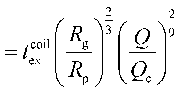 | (17) |
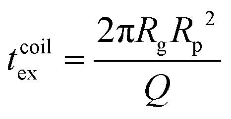 as the exit time of a non-deformed polymer coil.
Then, the ejection time ttheoej is calculated as the sum of the advection time of the polymer by the flow from the membrane to the ejection plane,
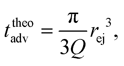 | (18) |
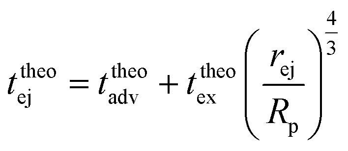 | (19) |
 | (20) |
Note that in this approach, we neglected the presence of other nanopores that will modify the flow field at long distances.
Effect of diffusion
Because of their sizes, the polymers are subject to diffusion. When an external flow is added, diffusion and advection compete with each other.27 To compute the diffusion coefficient of an elongated polymer in the de Gennes regime,28 one needs to take into consideration the contribution of each blob individually: | (21) |
And then the cooperative diffusion of Nb blobs forming the molecule is
 | (22) |
 | (23) |
Just like the ejection time, eqn (20), there are two contributions to the diffusion time of the molecule: the time taken by the tip of the molecule to diffuse to a plane at distance r, and the time taken by the whole length of the molecule to pass the plane at distance r. The first contribution is complex as the shape of the molecule changes with the distance to the nanopore. For simplicity, we consider, for the calculations of the diffusion time over a distance r, that the polymer molecule is a succession of blobs of size ξ(r/2) = ξ(r)/2. The total diffusion time to pass the plane at rej is then:
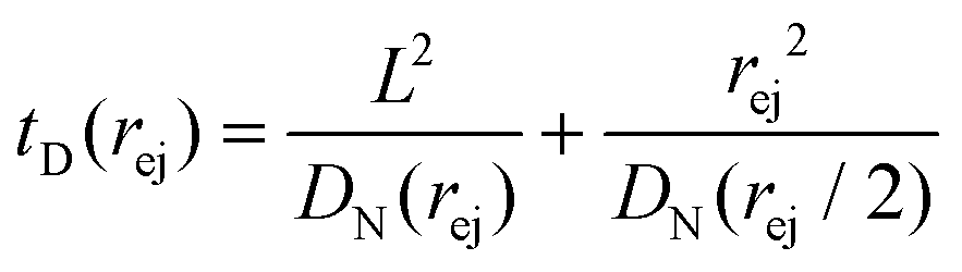 | (24) |
 | (25) |
The Peclet number that compares the relative influence of the advection and diffusion times is evaluated as:
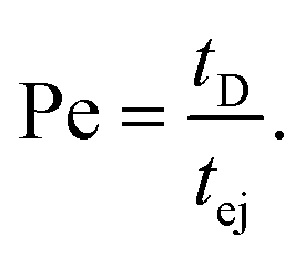 | (26) |
Numerical applications (see Tables 1 and 3) show that for the considered experimental conditions, the Peclet number of the large DNAs (T4 DNA and λ DNA) is always larger than one, which means that the transport time is governed by the advection times (exit time or ejection time). For the smaller DNAs, ΦX DNA and pNEB DNA, the Peclet number is smaller than one at low flow rates. In these cases, diffusion may play an important role in the transport of the molecules.
| Pore radius (nm) | ΔPc (mbar) | ΔP (mbar) | Pe |
|---|---|---|---|
| Each membrane is associated with a critical pressure gradient ΔPc, which only depends on the pore geometry.13 For each membrane, we explore a range of pressure gradients ΔP > ΔPc. The minimum Peclet number of the polymer is computed from eqn (26), using the lowest applied pressure. | |||
| 21 | 82 | 80–300 | 31–210 |
| 45 | 4 | 10–100 | 9.7–270 |
| 110 | 0.2 | 1–6 | 1.6–20 |
Influence of the flow field on DNA transport
Above a critical flow threshold, DNA molecules are deformed by the hydrodynamic shear stress. Following the affine model in an extensional flow outside of a nanopore, the molecule takes an elongated shape in the form of a series of beads with the radius increasing with their distance to the membrane. We expect the exit time to follow eqn (17), and the ejection time to follow eqn (20). The hydrodynamic stress exerted on the polymer depends on the imposed gradient of pressure, and the geometry of the nanopore. We conducted a series of experiments for a given polymer (λ DNA, Rg = 513 nm) on three different membranes with respective nanopore radius Rp = 21, 45 or 110 nm. Each membrane had a different critical pressure gradient ΔPc, and we probed a range of pressure gradients such that ΔP > ΔPc, and Pe > 1 (see Table 3).First, for the Rp = 45 nm nanopore membrane, the average intensity of all events at a given pressure gradient was considered while varying the pressure gradient (Fig. 4(a)). At low pressure (ΔP < 30 mbar), the intensities presented large fluctuations with time. These fluctuations are characteristics of diffusive behaviour. When the pressure gradient was increased, the duration of events (exit and ejection times) decreased, as expected for an object being transported by advection.
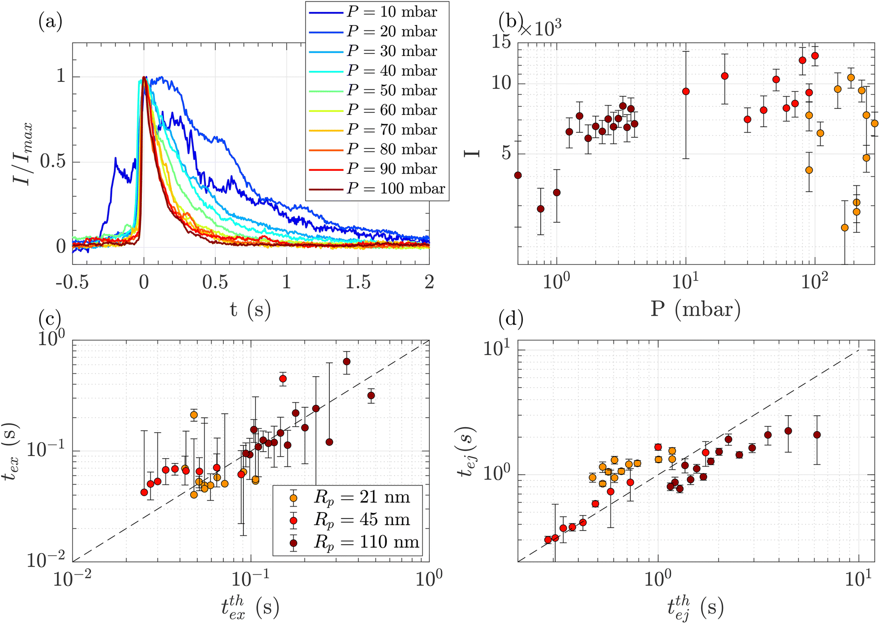 | ||
| Fig. 4 Characterisation of events for the translocation of λ DNA through membranes with nanopore radius Rp = 21, 45 or 110 nm, and at different pressures. (a) Normalised mean intensity of events for Rp = 45 nm, for different pressures ranging from P = 10 mbar (dark blue) to P = 100 mbar (dark red). The events are centred such that the intensity reaches its half height at t = 0 s. (b) Average of the intensity of all events at a given pressure and pore radius, as a function of the pressure. The colours correspond to the pore radius. (c) Exit times of the mean event for different pore radii versus theoretical exit time computed from the affine deformation model, eqn (17). The model does not require a fitting parameter. The black dashed line highlights the identity function. (d) Ejection times of the mean event intensity versus a theoretical ejection time computed from the affine deformation model, eqn (20). The fitting parameter, the position of the ejection plane, was evaluated to be rej = 6Rp. The black dashed line highlights the identity function. All error bars are computed from the standard deviation of the quantities measured on all events, divided by the square root of the number of events. If an error bar crosses zero on the logarithmic scale, it may be truncated. The dark red star indicates for reference the diffusion time on the characteristic distance rej, for the larger nanopores Rp = 110 nm. | ||
The maximum intensity of all events for different pressure gradients and different pore radii is shown in Fig. 4(b). The maximum intensity was widely distributed and showed no trend with pressure or the pore radius.
The exit and ejection times were measured for all events as described in the ‘Image processing’ section, from the evolution of intensity with time. They are shown in Fig. 4(c) and (d) as a function, respectively, of the theoretical exit time (eqn (17)) and the theoretical ejection time (eqn (20)). The exit time did not require any fitting parameter. The experimental measurement of the exit time collapsed on the line texpex = ttheoex.
The theoretical evaluation of the ejection time requires knowing the ejection plane, the plane beyond which the polymer is not optically detected anymore. The coordinate of this plane was determined by fitting the theoretical model with the experimental data. We then found a distance from the membrane rej = 6Rp, which is a very reasonable estimation, as the zero-mode waveguide has the maximum intensity near the membrane (at a distance of typically the radius of the nanopore, Rp), and then decays at longer distances. Using this fitting parameter, the experimental data collapsed on the line texpej = ttheoej.
These first sets of experiments using λ DNA, which is widely used in the literature, helped us validate the theoretical and experimental tools for the characterisation of translocation events.
Influence of the DNA molecular weight
DNA molecules of increasing molecular weights were expected to give both increasing intensities (increasing amount of fluorophores) and increasing characteristic times (as the radius of gyration and stretching length are also increasing). The translocation of DNA samples with four different molecular weights (see Table 1) was then compared through the same membrane (Rp = 45 nm, ΔPc = 4 mbar) and for pressure gradients ΔP ranging from 10 to 100 mbar. The average linear density of fluorophores being the same for all molecules, the intensity of an event was expected to increase with the molecular weight of the molecule, with an eventual non-linearity due to the GAIN of the camera. Indeed, this was observed in Fig. 5(a), displaying the distributions of the intensity of all events at all pressures for each DNA sample. Interestingly, while the smaller ΦX DNA presented a narrow distribution of intensity, for the larger DNA samples, the intensity distribution was broader, with a peak at high intensity and a slow tail toward low intensity.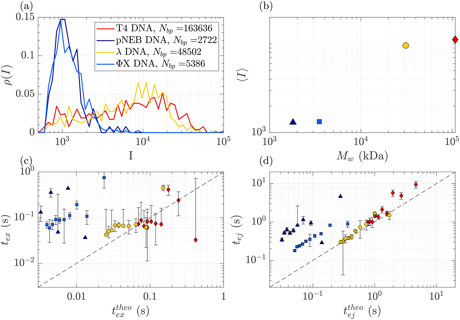 | ||
| Fig. 5 Characterisation of events for the translocation of DNA of different molecular weights through a Rp = 45 nm nanopore membrane, at different pressures ranging from ΔP = 10 mbar to 100 mbar. (a) Density of probability of event intensity for DNA solutions of T4 DNA, λ DNA, and ΦX DNA. (b) Evolution of the average intensity with the DNA molecular weight. (c) Exit times of the mean event intensity for different DNA molecular weights versus the theoretical exit time computed using the affine deformation model, eqn (17). The model did not require any fitting parameter. The black dashed line highlights the identity function. (d) Ejection times of the mean event intensity of different DNA molecular weights versus a theoretical ejection time computed from the affine deformation model, eqn (20). The same fitting parameter as the one determined in Fig. 4 was used. The black dashed line highlights the identity function. All error bars were computed from the standard deviation of the quantities measured on all raw events, divided by the square root of the number of events. If an error bar crosses zero on the logarithmic scale, it may be truncated. The stars indicate for reference the diffusion times on the characteristic distance rej, for each DNA. | ||
The average intensity for each DNA increased with the molecular weight of the DNA (Fig. 5(b)). Interestingly, the average maximum intensity of T4 DNA was only slightly higher than that of λ DNA, while their number of base pairs differs by a factor of 3. An explanation could be linked to the stretching of the larger DNA molecules across the illumination region. As one end of the DNA molecule is exiting the nanopore, the other end is advected away by the flow, getting less and less illumination. The distance to the ejection plane (rej, distance after which we stop detecting a signal, previously determined to be 6Rp = 0.76 μm) can be compared to the real length of a DNA molecule in the extensional flow (Table 1, see ESI S2, eqn (S5) and (S9)†). Typically, for λ, when one of its ends is at the nanopore and the other is at the ejection plane. The molecule is stretched over the whole illumination region. For the larger T4 DNA, part of the molecule may stretch beyond the ejection plane and thus may not add to the intensity signal detected by the camera. The maximum intensity signal corresponds to the portion of a stretched DNA across the illumination region.
In Fig. 5(c) and (d), the measured exit times and ejection times of all DNAs, for all events at all pressure gradients, are plotted as a function of the theoretical exit time (eqn (17), with no fitting parameter), and the theoretical ejection time (eqn (20), using the fitting parameter previously computed), respectively. The two larger DNAs, λ DNA and T4 DNA, collapsed on the lines texpex = ttheoex and texpej = ttheoej. Interestingly, the smaller ΦX DNA and pNEB DNA did not collapse on either line, and their transport times measured experimentally were higher than expected.
To understand this effect, we artificially rescaled the data for each molecular weight based on its value at P = 50 mbar, as illustrated in Fig. 6(a) and (b). The data then converged into the identity function. This observation suggests that the behaviour of small molecules is not attributed to a change in the regime (as the data still adhere to the same power law), but rather indicates that the model is lacking a component related to the dependence of a coefficient on the molecular weight of the molecule. This dependence can be assessed by calculating the ratio between the experimentally measured times and those obtained through the theoretical model, as depicted in Fig. 6(c). As expected the coefficients tend to converge to 1 for larger polymers and become significantly larger (up to nearly 100) for smaller polymers. The current experimental study cannot provide conclusive insights into the origin of these coefficients for small DNA molecules. We discuss further a plausible scenario based on the effect of diffusion in the ESI,† but a deeper understanding with further experimental investigation will be needed in the future for the development of a more comprehensive theoretical model.
 | ||
| Fig. 6 Rescaled characteristic times: (a) exit time and (b) ejection time for DNAs of various sizes. The data are from the same dataset as presented in Fig. 5, with the artificial removal of the offset achieved by rescaling each dataset based on its value at ΔP = 50 mbar. The dashed black lines represent the identity function. (c) The average ratio between the experimentally measured times and those obtained from the theoretical model for DNAs of various molecular weights, for the exit (in red) and ejection (in blue) times. | ||
Mixing two DNA populations
Given that some translocation characteristics of a DNA molecule depend on its molecular weight, such as the maximum intensity or the ejection time, we investigated whether these characteristics could be used to discriminate between two populations of DNA with different molecular weights, mixed in the same solution. We then prepared a series of DNA solutions with different volume fractions of the above-mentioned solutions of λ DNA (10 pM) and ΦX DNA (100 pM). To determine experimentally the relative proportion of each DNA, the total number of detected events was preferentially used rather than the initial concentration of DNA. Indeed, as the concentrations were very low, some significant amounts of DNA may be lost during the preparation process (for instance by adsorption on the vials and membrane). Instead, counting the event is a direct quantification of the number of molecules passing through the membrane.The distributions of the event maximum intensity for solutions of different volume fractions of λ DNA and ΦX DNA  are given in Fig. 7(a). On the one hand, rV = 1 (dark red) corresponded to the pure λ DNA solution, and presented a characteristic peak at Iλ = 104 a.u. On the other hand, rV = 0 (black) corresponded to the pure ΦX DNA solution, and presented a peak at IΦX = 103 a.u. These peaks were separated in the logarithmic representation. As expected, the solutions mixing the two DNA presented two peaks at Iλ and IΦX. The respective intensity of the peaks evolved in agreement with the volume fractions of the λ DNA and ΦX DNA solutions.
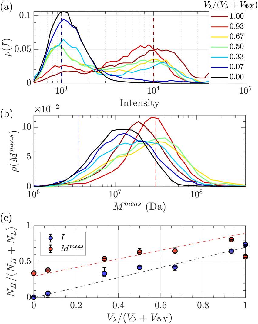 | ||
| Fig. 7 Characterisation of a solution of two DNAs of different molecular weights λ DNA and ΦX mixed at different volume fractions. (a) Density of probability of event intensity. The colour scale corresponds to the volume fraction of λ DNA molecules (red corresponds to 100% λ DNA, and dark blue to 100% ΦX DNA). (b) Density of probability of the apparent molecular weight, measured using eqn (20), and the experimental distribution of tej. Same colour scale as in (a). (c) In blue, the proportion of high-intensity events (around I = 104) compared to the sum of high-intensity events and low-intensity events (around I = 103), measured from the density of probability of the intensity in (a), versus the volume fraction of λ DNA in the solution. In red, the proportion of slow events (corresponding to Rg = Rg(λ)) compared to fast events (corresponding to Rg = Rg(Φ)X), measured from the density of probability of the measured molecular weight in (b) versus the volume fraction of λ DNA solution. The red dashed line with a slope of 0.6, and the black dashed line with a slope of 0.7 highlight the trends. The error bars were computed by computing the proportions using different probing boxes (50% to 150%) around the mean value of the pure solutions. | ||
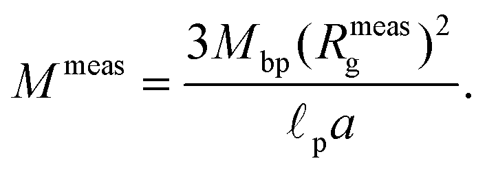
As fluorescence may be affected by the nature of the fluorophore and its environment, the intensity of translocation events cannot be used as such to compare the relative molecular weights of different objects. A more direct measurement to assess the molecular weight of a polymer is to consider its characteristic exit and ejection times. Because the exit time is shorter and more affected by diffusion, we focused on the ejection time to compute the apparent molecular weight of each event by inverting eqn (20).
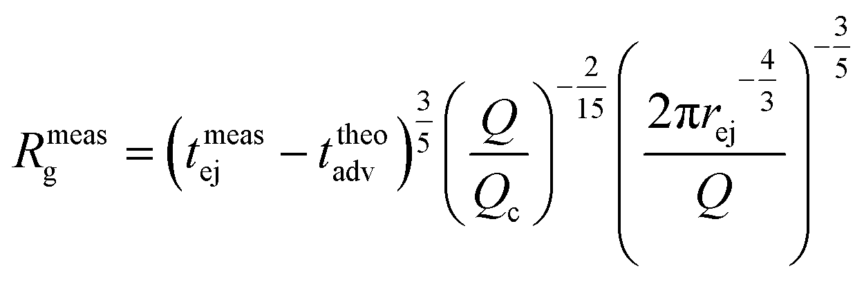 | (27) |
 | (28) |
meas = 11 MDa), relative to their volume fraction rV.
To go further, we computed the number of events presenting a maximum intensity or molecular weight close to either the first peak (denoted as L for low, indicated by a dashed blue line) or the second peak (denoted as H for high, indicated by a dashed red line). Typically, we defined a box between 0.8 to 1.2 around the peak position and event fraction 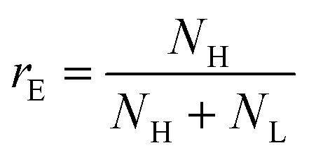 . In the event fraction versus volume fraction plot (Fig. 7(c)), the event fraction values computed both from the density of probability of intensity, and from the density of probability of the measured molecular weight, showed the same trend as that for the calibration curve, they increased linearly from a low value for pure ΦX DNA solution to a high value for pure λ DNA solution. To conclude, not only do both the maximum intensity and the ejection time give us information about the molecular weight of the molecule, but their distribution is related to the distribution of the molecular weight in the sample, and can be used to discriminate between two DNAs of different molecular weights in the same solution, and quantify their respective amount.
Transport of synthetic polymers
Our analytical tools were then applied to gather information about synthetic polymer samples that are, conversely to DNA, characterised by larger molecular weight distributions. Two high molecular weight poly(NAM-stat-NAS) copolymer skeletons were first synthesised by two different radical polymerisation methods: PolyHD was synthesised by conventional radical polymerisation, which leads to high dispersity samples (Đ = 3.6), and, PolyLD was synthesised by RAFT controlled polymerisation, which provides a much better control of the molecular weight and leads to a much lower dispersity (Đ = 1.4). The full SEC-MALLS chromatograms are given in the ESI, Fig. S2.† These two polymer skeletons were then identically grafted both with green-emitting fluorophores (see the SEC-UV chromatogram in the ESI, Fig. S4†) and with 2 kDa PEG branches (the full structure of the molecule is given in the ESI, in Fig. S1†). The latter increase the radius of gyration of the polymer and limit the effect of diffusion (see Table 4). Finally, two polymer samples were obtained with a similar number-average molecular weight (Mn = 0.5–0.6 MDa). However, because of its high dispersity, PolyHD weight-average molecular weight (Mw = 1.9 MDa) was much higher than that of PolyLD (Mw = 0.9 MDa).| PolyHD | PolyLD | |
|---|---|---|
 and and 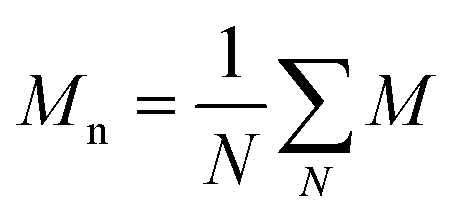 are respectively the weight-average and number-average molecular weights determined by SEC-MALLS for the poly(NAM-stat-NAS) skeletons and calculated for the branched polymers. are respectively the weight-average and number-average molecular weights determined by SEC-MALLS for the poly(NAM-stat-NAS) skeletons and calculated for the branched polymers. 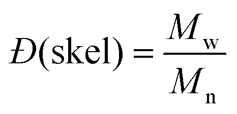 is the dispersity of the samples determined by SEC-MALLS. The radius of gyration Rg of poly(NAM-stat-NAS) skeletons was computed using the Flory approximation in a good solvent:29Rg(skel) = aN0.59, where a = 300 pm is the size of a monomer and N the number of monomers computed from Mn. Rg of grafted polymers was computed as:30 is the dispersity of the samples determined by SEC-MALLS. The radius of gyration Rg of poly(NAM-stat-NAS) skeletons was computed using the Flory approximation in a good solvent:29Rg(skel) = aN0.59, where a = 300 pm is the size of a monomer and N the number of monomers computed from Mn. Rg of grafted polymers was computed as:30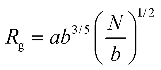 , where N is the total number of monomers (branches + skeleton), and b = 4 is the number of monomers on the skeleton between two branches. Here, the monomers of the branches (CH2–CH2–O–) are different from the ones of the skeleton (C–C bonds). As the former are in excess, we chose as an approximation to consider that all monomers have the size of a PEG monomer a = 440 pm (Rg value changes by a factor 0.7 by using instead a skeleton monomer). The mean intensity in number , where N is the total number of monomers (branches + skeleton), and b = 4 is the number of monomers on the skeleton between two branches. Here, the monomers of the branches (CH2–CH2–O–) are different from the ones of the skeleton (C–C bonds). As the former are in excess, we chose as an approximation to consider that all monomers have the size of a PEG monomer a = 440 pm (Rg value changes by a factor 0.7 by using instead a skeleton monomer). The mean intensity in number  and the mean intensity in weight and the mean intensity in weight 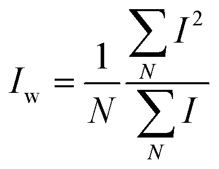 are measured directly on the distribution given Fig. 8(c). The intensity dispersity are measured directly on the distribution given Fig. 8(c). The intensity dispersity 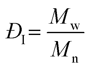 is the average of the intensity dispersity of several independent experiments. For the intensity dispersity, an average was done on several experiments and an incertitude was derived from the standard deviation in the measures. The individual measurements from the intensity distribution of each realisation are given in the ESI S5 Tables S1 and S2.† is the average of the intensity dispersity of several independent experiments. For the intensity dispersity, an average was done on several experiments and an incertitude was derived from the standard deviation in the measures. The individual measurements from the intensity distribution of each realisation are given in the ESI S5 Tables S1 and S2.† |
||
| M w(skel) | 0.50 MDa | 0.23 MDa |
| M n(skel) | 0.14 MDa | 0.17 MDa |
| Đ(skel) | 3.58 | 1.35 |
| R g(skel) | 20 nm | 22 nm |
| M w(grafted) | 1.88 MDa | 0.86 MDa |
| M n(grafted) | 0.52 MDa | 0.63 MDa |
| R g(grafted) | 56 nm | 62 nm |
| I n | 1.88 × 10³ | 1.70 × 10³ |
| I w | 2.54 × 10³ | 1.94 × 10³ |
| Đ I | 1.44 ± 0.22 | 1.18 ± 0.04 |
Translocation events through the Rp = 45 nm membrane were indeed detected for both polymers and the average event intensity was measured at different pressures following the same method as that for the DNA molecules, except for the use of a higher gain for the camera (Fig. 8(a) for PolyLD). Events exhibited a similar shape to the one previously observed with DNA, with an exiting phase when the polymer is leaving the nanopore, and an ejection time when the polymer is advected by the flow away from the nanopore. While the exit time was too short to be measured in this case, a decrease in the ejection time was again observed with the increasing pressure gradient. In Fig. 8(b), we compared these times with the pure advection time of a polymer coil through the illumination region. The polymers were transported by the extensional flow with little deformation. The Pe of a coil polymer molecule of size Rg can be computed from its advection time 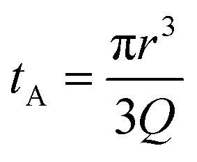 and diffusion time
 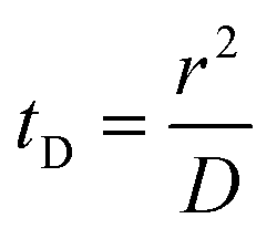 :
:
 | (29) |
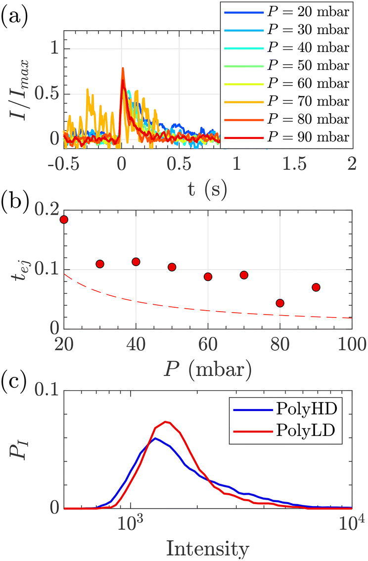 | ||
| Fig. 8 Characterisation of events for the translocation of synthetic polymers with similar number-average molecular weight but different dispersity through Rp = 45 nm membranes, and at different pressures. (a) Normalised mean intensity of events of PolyLD (low dispersity), for different pressures ranging from P = 20 mbar (dark blue) to P = 90 mbar (dark red). The signal has been smoothed using a mean filter for better visualisation. The events are centred such that the intensity reaches its half height at t = 0 s. (b) Ejection times measured from the mean intensity of a translocation event for PolyLD (low dispersity) at different pressures. The black dashed line shows the value of the theoretical diffusion time tD (eqn (25)) over a distance rej, and the red dashed line shows the sum of the theoretical diffusion and ejection (eqn (20)) time tD + tej. (c) Density of probability of event intensity for the two synthetic polymers. | ||
At a given pressure gradient (for instance ΔP = 20 mbar), the Peclet number of a short polymer molecule Mw = 0.1 MDa, Rg = 48 nm is Pe = 0.44, and the Peclet number of a long polymer molecule Mw = 1 MDa, Rg = 150 nm is Pe = 1.4. Diffusion is expected to play a role, and even be predominant at low flow rates or low molecular weights. The theoretical model slightly underestimated the experimental values, which might also be explained by the role played by diffusion in the exploration of longer trajectories, as proposed for the small DNA molecules. For these reasons, we thus chose to use the event intensities to compare the molecular weight dispersity of both synthetic polymers.
We plotted the density of probability of the intensity of all events for the two polymers (Fig. 8(c)). The molecular weight distributions of polymer samples as measured by SEC-MALLS (Fig. S3†) are typically described by the number-average molecular weight Mn, the weight-average molecular weight Mw, and the dispersity Đskel. By analogy, we defined similar characteristics for intensity distributions: the number-average intensity In, the intensity-average intensity Iw, and the intensity dispersity Đ (Table 4). Based on several experiments, the intensity distributions indeed reproducibly captured the difference in dispersity between PolyHD and PolyLD (Fig. 8(c)). This difference in the intensity distributions remained nonetheless lower than the one measured by SEC-MALLS, which is likely due to the lack of accuracy in capturing the translocation events corresponding to the low molecular weight fraction of the polymer samples. Still, those results are very encouraging for the future development of the technique for the characterisation of synthetic polymers.
Conclusion
The zero-mode waveguide for the nanopore technique has been used previously to study the transport of biomolecules and viral particles.7,11,14–17 In this work, we developed a series of tools to characterise the translocation of a polymer through a nanopore. In particular, we measure the characteristic time of a translocation event. For double-stranded DNA, when the molecule is large enough so that the role of diffusion is negligible under the experimental conditions we considered, the experimental measurements are in perfect agreement with a classical theoretical model considering the affine deformation of the molecule in the flow. When diffusion starts to play a role, we observe that the molecules’ transport time becomes longer than expected. We propose an explanation based on the de-centering of the polymer in the pore due to diffusion, which causes the molecule to follow longer trajectories before exiting the illumination plane. The experimental measurement of the intensity or characteristic times of events enables us to go back to the distribution of an apparent molecular weight. Using these distributions we are able to discriminate two DNA populations in a solution, and quantify their respective volume fraction. Finally, applying these same tools for smaller synthetic polymers, we were able to retrieve information on their molecular weight distribution that varied depending on their synthesis method.From the range of measurements conducted on different objects, various physical questions arose. Because this paper presents a set of tools, we chose not to focus on one question but present some potential applications. The tools we developed can now be used to investigate technical questions such as the influence of fluorophore densities on the backbone or the influence of fluorescence quenching.
For shorter polymers, the technique we presented is essentially limited by the acquisition time scale and signal-to-noise ratio of the camera. Sensors based on a single photodiode (SPD)7 have been shown to increase the frame rate but without parallelisation. The development of SPD arrays will lead, in the coming years, to better resolved and high throughput detection based on the same approach. Finally, for the next step, we would like to develop the current optical set-up to be able to sequence complex objects, for instance, to achieve the high flow rate reading of barcoded DNA31 and polymers.
Author contributions
F. Montel and A. Favier initiated and supervised the project. B. Molcrette conducted preliminary transport experiments on synthetic polymers. C. de Blois developed the experimental protocol, conducted the experimental investigation of DNA and synthetic polymers and performed image analysis. F. Montel and C. de Blois built the theoretical model of polymer transport. A. Favier designed the structure of the synthetic polymers. M.-A. Rejou and M. Engel performed the synthesis of the polymers. C. de Blois, F. Montel and A. Favier wrote the manuscript. All the authors participated in the scientific discussions.Conflicts of interest
There are no conflicts to declare.Acknowledgements
This work was supported by the LABEX iMUST (ANR-10-LABX-0064) of Université de Lyon, within the program “Investissements d'Avenir” (ANR-11-IDEX-0007) operated by the French National Research Agency (ANR). The authors sincerely thank Vincent Demery for the valuable theoretical insights and a thorough review of our paper. His input has been instrumental in enhancing the quality of our work. The authors are also thankful for the help of Saskia Brugere in the characterisation of the DNA used in the study. We acknowledge Agnès Crépet as well as the facility and expertise of the Liquid Chromatography of polymer platform of Institut de Chimie de Lyon, ICL (FR5223) for technical support in SEC/MALLS characterisation.Notes and references
- M. I. Giannotti and G. J. Vancso, Interrogation of single synthetic polymer chains and polysaccharides by AFM-based force spectroscopy, ChemPhysChem, 2007, 8(16), 2290–2307 CrossRef CAS.
- J. W. Black, M. Kamenetska and Z. Ganim, Nano Lett., 2017, 17, 6598–6605 CrossRef CAS PubMed.
- M. Wanunu, J. Sutin, B. McNally, A. Chow and A. Meller, Biophys. J., 2008, 95, 4716–4725 CrossRef CAS PubMed.
- P. Bandarkar, H. Yang, R. Henley, M. Wanunu and P. C. Whitford, Biophys. J., 2020, 118, 1612–1620 CrossRef CAS.
- C. Plesa, S. W. Kowalczyk, R. Zinsmeester, A. Y. Grosberg, Y. Rabin and C. Dekker, Nano Lett., 2013, 13, 658–663 CrossRef CAS.
- G. Baaken, N. Ankri, A. K. Schuler, J. Rühe and J. C. Behrends, ACS Nano, 2011, 5, 8080–8088 CrossRef CAS.
- N. Klughammer and C. Dekker, Nanotechnology, 2021, 32, 18LT01 CrossRef CAS PubMed.
- A. Zrehen, D. Huttner and A. Meller, ACS Nano, 2019, 13, 14388–14398 CrossRef CAS PubMed.
- M. Boukhet, N. F. König, A. A. Ouahabi, G. Baaken, J. Lutz and J. C. Behrends, Macromol. Rapid Commun., 2017, 38, 1700680 CrossRef PubMed.
- A. Ivankin, R. Y. Henley, J. Larkin, S. Carson, M. L. Toscano and M. Wanunu, ACS Nano, 2014, 8, 10774–10781 CrossRef CAS.
- T. Gilboa and A. Meller, Analyst, 2015, 140, 4733–4747 RSC.
- C. Plesa, L. Cornelissen, M. W. Tuijtel and C. Dekker, Nanotechnology, 2013, 24, 475101 CrossRef.
- T. Auger, J. Mathé, V. Viasnoff, G. Charron, J.-M. Di Meglio, L. Auvray and F. Montel, Phys. Rev. Lett., 2014, 113, 028302 CrossRef CAS.
- L. Chazot-Franguiadakis, J. Eid, M. Socol, B. Molcrette, P. Guégan, M. Mougel, A. Salvetti and F. Montel, Nano Lett., 2022, 22, 3651–3658 CrossRef CAS.
- P. J. Kolbeck, D. Benaoudia, L. Chazot-Franguiadakis, G. Delecourt, J. Mathé, S. Li, R. Bonnet, P. Martin, J. Lipfert, A. Salvetti, M. Boukhet, V. Bennevault, J.-C. C. Lacroix, P. Guégan and F. Montel, Nano Lett., 2023, 23, 4862–4869 CrossRef CAS PubMed.
- B. Molcrette, L. Chazot-Franguiadakis, F. Liénard, Z. Balassy, C. Freton, C. Grangeasse and F. Montel, Proc. Natl. Acad. Sci. U. S. A., 2022, 119, e2202527119 CrossRef CAS.
- C. Shasha, R. Y. Henley, D. H. Stoloff, K. D. Rynearson, T. Hermann and M. Wanunu, ACS Nano, 2014, 8, 6425–6430 CrossRef CAS.
- M. J. Levene, J. Korlach, S. W. Turner, M. Foquet, H. G. Craighead and W. W. Webb, Science, 2003, 299, 682–686 CrossRef CAS PubMed.
- C. Cepraga, T. Gallavardin, S. Marotte, P.-H. Lanoë, J.-C. Mulatier, F. Lerouge, S. Parola, M. Lindgren, P. L. Baldeck, J. Marvel, O. Maury, C. Monnereau, A. Favier, C. Andraud, Y. Leverrier and M.-T. Charreyre, Polym. Chem., 2013, 4, 61–67 RSC.
- A. Favier, F. D'Agosto, M.-T. Charreyre and C. Pichot, Polymer, 2004, 45, 7821–7830 CrossRef CAS.
- C. Gaillot, F. Delolme, L. Fabre, M.-T. Charreyre, C. Ladavière and A. Favier, Anal. Chem., 2020, 92, 3804–3809 CrossRef CAS.
- C. Cepraga, A. Favier, F. Lerouge, P. Alcouffe, C. Chamignon, P.-H. Lanoë, C. Monnereau, S. Marotte, E. Ben Daoud, J. Marvel, Y. Leverrier, C. Andraud, S. Parola and M.-T. Charreyre, Polym. Chem., 2016, 7, 6812–6825 RSC.
- W. Reisner, J. N. Pedersen and R. H. Austin, Rep. Prog. Phys., 2012, 75, 106601 CrossRef PubMed.
- L. Béguin, B. Grassl, F. Brochard-Wyart, M. Rakib and H. Duval, Soft Matter, 2011, 7, 96–103 RSC.
- P. G. de Gennes, Scaling Concepts in Polymer Physics, Cornell University Press, 1979 Search PubMed.
- S. Daoudi and F. Brochard, Macromolecules, 1978, 11, 751–758 CrossRef CAS.
- M. Muthukumar, Polymer Translocation, CRC Press, 2016 Search PubMed.
- F. Brochard and P. G. de Gennes, J. Chem. Phys., 1977, 67, 52–56 CrossRef CAS.
- J. Isaacson and T. Lubensky, J. Phys., Lett., 1980, 41, 469–471 CrossRef CAS.
- T. Sakaue and F. Brochard-Wyart, ACS Macro Lett., 2014, 3, 194–197 CrossRef CAS.
- V. Pan, W. Wang, I. Heaven, T. Bai, Y. Cheng, C. Chen, Y. Ke and B. Wei, ACS Nano, 2021, 15, 15892–15901 CrossRef CAS PubMed.
Footnote |
| † Electronic supplementary information (ESI) available: S1: Movie, observation of the translocation of λ DNA through nanopores Rp = 45 nm. S2: Model of the real length of a molecule at the exit of a nanopore (eqn (S1)–(S9)). S3: Complementary information on the structure and characterisation of synthetic polymers (Fig. S1 to S4). S4: Complementary discussion on the effect of diffusion on the transport of small molecules. S5: Complementary data for the measure of the dispersity of synthetic polymer samples (Tables S1 and S2). See DOI: https://doi.org/10.1039/d3nr04915a |
| This journal is © The Royal Society of Chemistry 2024 |