
 Open Access Article
 This Open Access Article is licensed under a Creative Commons Attribution-Non Commercial 3.0 Unported Licence
Preparation and characterization of highly crystalline hydroxyapatite (HAp) from the scales of an anadromous fish (Tenualosa ilisha): a comparative study with the freshwater fish scale (Labeo rohita) derived HAp†
Mashrafi Bin Mobarak *a,
Fariha Chowdhuryb and
Samina Ahmed*a
*a,
Fariha Chowdhuryb and
Samina Ahmed*a
aInstitute of Glass and Ceramic Research and Testing (IGCRT), Bangladesh Council of Scientific and Industrial Research (BCSIR), Dhaka-1205, Bangladesh. E-mail: mashrafibinmobarak@gmail.com; shanta_samina@yahoo.com
bBiomedical and Toxicological Research Institute (BTRI), Bangladesh Council of Scientific and Industrial Research (BCSIR), Dhaka-1205, Bangladesh
First published on 18th December 2024
Abstract
Waste generation from fish processing sectors has become a significant environmental concern. This issue is exacerbated in countries with high aquaculture production and inefficient fish scale (FS) utilization. This study prepared and compared highly crystalline hydroxyapatite (HAp) from the FS of an anadromous fish, Tenualosa ilisha (I-HAp), and a freshwater fish, Labeo rohita (R-HAp). Acid–alkali treatment followed by high-temperature calcination was employed for HAp synthesis. XRD analysis indicated a monoclinic crystal structure for I-HAp and a hexagonal structure for R-HAp, with both containing β-TCP as a secondary phase. Rietveld refinement quantified β-TCP at 8% for I-HAp and 7.2% for R-HAp. Crystallite size of the samples was estimated by various methods (Scherrer's method, Scherrer equation average method, linear straight-line method, straight line passing the origin method, Monshi–Scherrer method, Halder–Wagner method, Williamson–Hall method, and size–strain plot method), consistently indicating microcrystalline HAp. FESEM and TEM analyses revealed larger particle sizes for I-HAp, confirmed by DLS measurements. Surface elemental analysis by XPS confirmed the presence of Na and Mg as impurities along with the elements of the HAp structure. FTIR and Raman spectroscopy identified expected functional groups, while EDX determined elemental composition. Both HAp samples exhibited bioactivity through apatite layer formation in simulated body fluid. Furthermore, the combined results of the cell viability and hemocompatibility studies indicate the biocompatibility of the prepared samples.
1. Introduction
Hydroxyapatite (HAp), with the chemical formula Ca10(PO4)6(OH)2, is a naturally occurring mineral form of calcium phosphate and the primary inorganic component of bone and teeth.1,2 Structurally, HAp crystallizes in a hexagonal or monoclinic system, characterized by a lattice structure that includes calcium ions occupying larger cationic sites and phosphate ions in smaller anionic sites, forming a robust framework essential for its biological functions. The hexagonal structure is more commonly associated with biological apatite, while the monoclinic form is often observed in synthetic HAp.3 The specific structure can influence properties like solubility, bioactivity, and mechanical behavior. The stoichiometric ratio of calcium to phosphate in HAp is approximately 1.67, which closely resembles the composition of natural bone, contributing to its excellent biocompatibility, osteoconductivity, and bioactivity.4,5 HAp's unique properties make it highly valuable in various biomedical applications, including bone tissue engineering,6 orthopedic implants,7 and drug delivery systems.8 The increasing importance of HAp in medicine stems from its ability to mimic the natural mineral phase of bone, making it a preferred material for implants and grafts.9 Its versatility allows for modifications, such as doping with other elements to enhance specific properties, thus broadening its applications in both human health and environmental applications.10,11HAp can be synthesized through various methods, including wet chemical precipitation,12 solid-state reactions,13,14 hydrothermal processes,15 and microwave-assisted techniques.16 The wet chemical method is particularly prevalent, where calcium and phosphate sources are mixed in solution to precipitate HAp at controlled pH and temperature conditions. Solid-state synthesis involves high-temperature reactions between calcium and phosphate powders, while hydrothermal synthesis utilizes water at elevated temperatures and pressures to produce highly crystalline HAp. Microwave-assisted synthesis is a rapid method that employs microwave energy to achieve uniform heating, resulting in smaller particle sizes and improved purity of HAp. In recent years, utilizing waste materials for HAp synthesis has gained attention due to environmental and economic benefits. This approach not only reduces waste but also provides a cost-effective source of calcium and phosphate. For instance, waste from agricultural products, such as eggshells and mussel shells, has been successfully converted into HAp, demonstrating comparable properties to synthetic HAp. This method not only addresses waste management issues but also promotes sustainability in material production.17 Specifically, the synthesis of HAp from fish scales has emerged as a promising technique. Fish scales are protective structures that cover the outer layer of a fish's body. These mineralized plates are primarily composed of organic and inorganic materials. Approximately 41–45% of fish scales consist of organic substances like collagen, fats, and vitamins, while the remaining portion comprises inorganic minerals such as calcium-deficient hydroxyapatite, calcium phosphate, and trace elements including magnesium, iron, and zinc.18 HAp can be extracted from fish scales using several methods. Common techniques include thermal treatment,19 alkaline or acidic treatment,20 and microwave irradiation.21 Thermal treatment involves heating fish scales at high temperatures to decompose organic matter, leaving behind HAp. Alkaline heat treatment uses a solution of alkali and/or acid, such as NaOH or HCl, to dissolve organic components and isolate HAp. Microwave irradiation accelerates the process by using microwaves to heat the scales and extract HAp.
Bangladesh currently stands 5th in the world aquaculture production with a production of 4.759 million MT in the FY 2021–2022, according to the annual report published in 2023 by department of fisheries, Bangladesh.22 Fish scale accounts for approximately 3% of the total weight and based on this approximation, 0.143 million MT of fish scales was generated in the FY 2021–2022. Around 30% of this fish scales are utilized, mostly by exporting to countries like Japan, China, and Thailand. The export of fish scales has become a burgeoning industry, with revenues reaching approximately 24 million USD annually.23 Meanwhile, a staggering 70% remains unutilized, highlighting a substantial waste management issue. Local fish processors and traders are increasingly recognizing the economic potential of fish scales, which are rich in collagen and can be transformed into valuable products such as biomaterials and gelatin for the healthcare, food and cosmetics industries. However, despite this potential, a significant portion of fish scales continues to be discarded, resulting in environmental pollution and lost economic opportunities, underscoring the need for better waste management practices and commercial utilization strategies in the country.24
Hilsa, an anadromous fish and the national fish of Bangladesh, constitutes 11% of the total fish production, contributes 1% to the country's GDP, and generates foreign exchange through exports.25 Among the five Hilsa species, Tenualosa ilisha is the most common, migrating from the Bay of Bengal into rivers like the Padma and Meghna.26,27
This study pioneers the preparation of HAp from Tenualosa ilisha scales using acid-alkali treatment and high-temperature calcination. A comparative analysis was conducted with HAp derived from the scales of Labeo rohita, a freshwater fish. Comprehensive characterization was performed to elucidate the properties of both HAp samples, and their bioactivity was assessed.
2. Materials and methods
2.1 Materials
Fish scales were collected from Jatrabari fish market, Dhaka, Bangladesh. HAp was prepared from both fish sources by treating the FS with acid and base solutions. Hydrochloric acid (HCl) and sodium hydroxide (NaOH) (both from Merck, Germany) were used for this purpose. All experiments were conducted using deionized (DI) water.2.2 Methods
![[thin space (1/6-em)]](https://www.rsc.org/images/entities/char_2009.gif) :2.5 ratio (fish scale weight in grams:HCl volume in milliliters) to deproteinize the scales.28 The mixture was stirred vigorously for 10–15 minutes and then left to soak in the acid solution for 24 hours at room temperature (25 ± 1 °C). Following the soaking period, the acid solution was decanted, and the scales were washed three times with DI water (150 mL each time) using vigorous stirring. The washed scales were subsequently treated with a 1 N NaOH solution, adhering to a 1:2.5 ratio (initial fish scale weight in grams:NaOH volume in milliliters). This basic treatment involved vigorous stirring for 10–15 minutes, followed by soaking for 24 hours at room temperature. The base solution was decanted; the scales were washed three times with DI water, and then boiled for 30 minutes at 80 °C. After another washing cycle, the scales were oven-dried at 80 °C for four hours. The dried scales underwent calcination at 1000 °C for three hours, with a temperature increase rate of 10 °C min−1, to obtain crystalline HAp. Both Tenualosa ilisha and Labeo rohita FS were processed concurrently using this methodology. The resulting HAp is referred to as I-HAp and R-HAp, respectively.
:2.5 ratio (fish scale weight in grams:HCl volume in milliliters) to deproteinize the scales.28 The mixture was stirred vigorously for 10–15 minutes and then left to soak in the acid solution for 24 hours at room temperature (25 ± 1 °C). Following the soaking period, the acid solution was decanted, and the scales were washed three times with DI water (150 mL each time) using vigorous stirring. The washed scales were subsequently treated with a 1 N NaOH solution, adhering to a 1:2.5 ratio (initial fish scale weight in grams:NaOH volume in milliliters). This basic treatment involved vigorous stirring for 10–15 minutes, followed by soaking for 24 hours at room temperature. The base solution was decanted; the scales were washed three times with DI water, and then boiled for 30 minutes at 80 °C. After another washing cycle, the scales were oven-dried at 80 °C for four hours. The dried scales underwent calcination at 1000 °C for three hours, with a temperature increase rate of 10 °C min−1, to obtain crystalline HAp. Both Tenualosa ilisha and Labeo rohita FS were processed concurrently using this methodology. The resulting HAp is referred to as I-HAp and R-HAp, respectively.3. Results and discussion
3.1 X-ray powder diffraction study
The preparation of HAp from Tenualosa ilisha and Labeo rohita FS sources was confirmed through the XRD analysis. The XRD patterns of I-HAp and R-HAp are shown in Fig. 1. | ||
| Fig. 1 XRD patterns of the prepared HAp from scales of (a) Tenualosa ilisha and (b) Labeo rohita. | ||
The XRD patterns indicate the presence of both HAp and beta-tricalcium phosphate (β-TCP) phases, suggesting a bi-phasic material. Confirmation was achieved by matching the patterns with standard ICDD (International Centre for Diffraction Data) database. The HAp prepared from Tenualosa ilisha FS had the closest match with ICDD PDF card #01-076-0694.30 Interestingly, the sharpest peak of I-HAp was seen at diffraction angle of 25.97° that corresponds to the (0 0 2) plane and the ICDD PDF card shows the I-HAp to be of monoclinic structure that belongs to the space group P21/b (14).
The most intense and characteristic peaks of HAp observed in the XRD patterns of I-HAp are: 10.94°, 31.89°, 32.29°, 33.02°, 34.16°, 39.91°, 46.79°, 49.58° and 53.28° which corresponds to the crystal plane of (1 0 0), (2 2 1), (−2 2 2), (−3 6 0), (−2 4 2), (−3 8 0), (−2 8 2), (−1 6 3) and (0 0 4). Presence of β-TCP as secondary phase was also confirmed through the search and matching operation (ICDD PDF card #04-010-2972).31 The secondary β-TCP phase is assigned to the peaks and planes at 31.32° (−2 2 −10), 32.67° (−3 1 8), 41.08° (−4 4 4), 42.11° (−3 3 12), 57.23° (−4 4 16), 60.04° (−6 2 10) and 60.52° (−5 2 −16). For the case of R-HAp, the XRD pattern had the closest match with ICDD PDF card #01-074-0565.32 Sharpest peak of R-HAp was seen at diffraction angle of 31.80° that corresponds to the (2 1 1) plane and the ICDD PDF card shows the R-HAp to be of hexagonal structure that belongs to the space group P63/m (176). The most significant and characteristic peaks of HAp that were observed in the XRD pattern of R-HAp are: 10.86°, 25.88°, 31.80°, 32.20°, 32.94°, 34.08°, 39.84°, 46.72° and 49.48°. The corresponding crystal plane of these diffraction angles are: (1 0 0), (0 0 2), (2 1 1), (1 1 2), (3 0 0), (2 0 2), (1 3 0), (2 2 2) and (2 1 3) respectively. Existence of secondary phase of β-TCP was also detected which corresponds to the ICDD PDF card #04-008-8714.33 Observed peaks of β-TCP and their corresponding crystal planes were 31.13° (−2 2 −10), 32.64° (−3 1 8), 33.82° (−2 2 12), 42.03° (−3 3 12), 57.12° (−5 5 −10) and 59.97° (−6 2 10).
| Sample | % of HAp | % of β-TCP | Rwp | Rexp | χ2 | GoF |
|---|---|---|---|---|---|---|
| a Here, Rwp = weighted profile residual, Rexp = expected profile residual, χ2 = ratio of Rwp2/Rexp2, and GoF = goodness of fit. | ||||||
| I-HAp | 92.0 | 8.0 | 13.18 | 17.31 | 0.5797 | 0.7614 |
| R-HAp | 92.8 | 7.2 | 13.99 | 17.18 | 0.6631 | 0.8143 |
The results of Rietveld refinement of the prepared samples reveal the amount of HAp and β-TCP phases present. R-HAp has a slightly higher percentage of β-TCP (7.2%) compared to I-HAp (8.0%). The Rietveld-refined XRD patterns obtained using the Profex software is shown in Fig. 2.
 | ||
| Fig. 2 Rietveld refinement of XRD patterns of (a) I-HAp and (b) R-HAp. | ||
Lattice parameter equation for the monoclinic I-HAp and hexagonal R-HAp is given by the eqn (1) and (2),14,34
 | (1) |
 | (2) |
Volume of unit cell (V) for monoclinic I-HAp and hexagonal R-HAp is given by the eqn (3) and (4),35,36
|
V = abcsinβ
| (3) |
 | (4) |
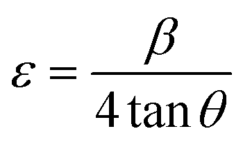
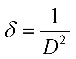
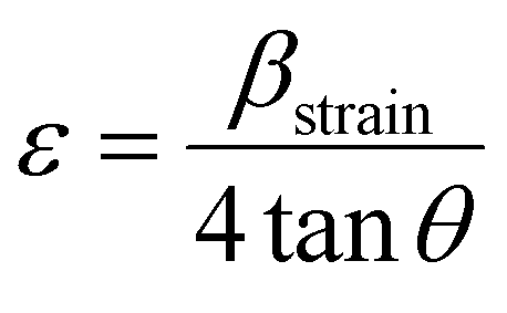
Density of unit cell (ρ), micro-strain (ε), and dislocation density (δ) are represented by eqn (5)–(7) respectively,
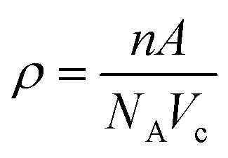 | (5) |
 | (6) |
 | (7) |
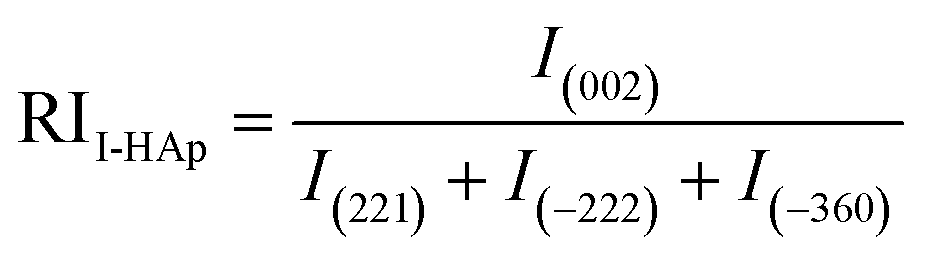
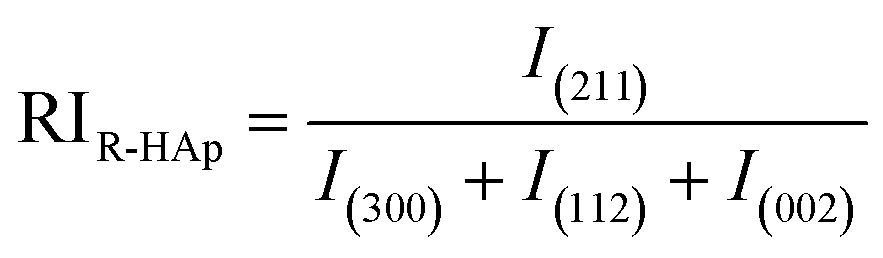
Relative intensity (RI) of I-HAp and R-HAp was calculated using eqn (8) and (9) and the preference growth was calculated using eqn (10),37
 | (8) |
 | (9) |
 | (10) |
The preference growth of I-HAp along the (002) plane and R-HAp along the (211) plane was calculated by considering their relative intensity along these planes. The RI of I-HAp was calculated by comparing the intensity of (002) plane against the next three most intense planes (221), (−222) and (−360). Similarly, RI of R-HAp was calculated by comparing (211) plane against the next three most intense planes (300), (112) and (002). The standard RI of I-HAp (0.52) and R-HAp (1.06) was found from their respective ICDD PDF card.
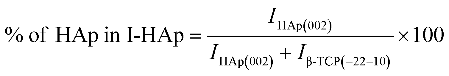
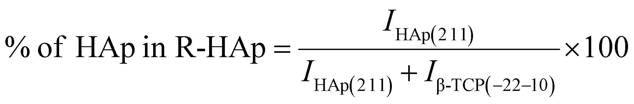
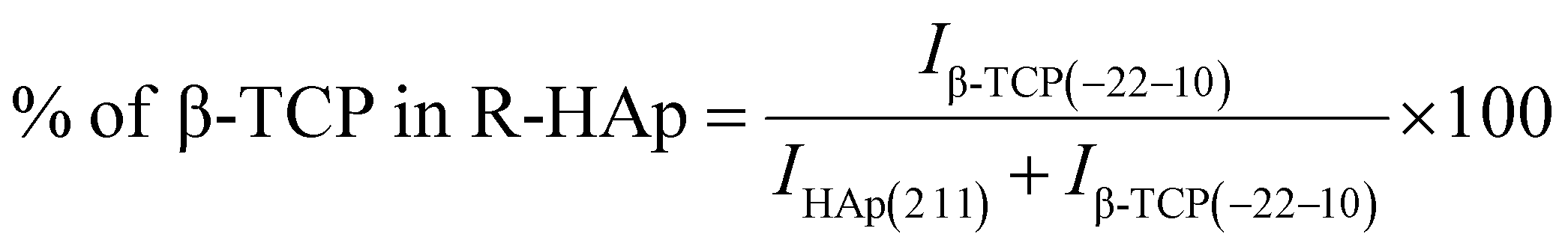
The theoretical percentage of HAp and β-TCP present in I-HAp was calculated using eqn (11) and (12), whereas eqn (13) and (14) represents the same for R-HAp,12
 | (11) |
 | (12) |
 | (13) |
 | (14) |
Volume fraction of β-TCP (XB) and degree of crystallinity (XC) of both I-HAp and R-HAp were calculated using eqn (15) and (16) respectively,12
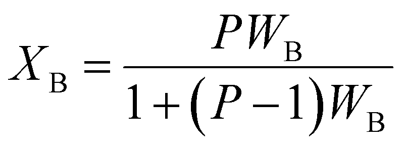 | (15) |
 | (16) |
| Parameters | I-HAp | ICDD PDF card #01-076-0694 | R-HAp | ICDD PDF card #01-074-0565 |
|---|---|---|---|---|
| Unit cell dimensions (Å) | a = 8.08, b = 16.32, c = 6.86 | a = 9.42, b = 18.84, c = 6.88 | a = b = 9.41, c = 6.88 | a = b = 9.42, c = 6.88 |
| Volume of unit cell (Å3) | 904.24 | 1057.96 | 527.64 | 529.09 |
| Density of unit cell (g cm−3) | 3.69 | 3.15 | 3.16 | 3.15 |
| Micro-strain | 0.07 | — | 0.06 | — |
| Relative intensity | 0.51 | 0.52 | 0.57 | 1.06 |
| Preference growth | −0.02 | — | −0.46 | — |
| % of HAp | 95.5 | — | 94.46 | — |
| % of β-TCP | 4.5 | — | 5.54 | — |
| Volume fraction of β-TCP | 0.10 | — | 0.11 | — |
| Degree of crystallinity | 50.81 | — | 52.73 | — |
Based on the obtained crystallographic parameters, the crystal structure of I-HAp and R-HAp was created using the VESTA 3 software and is presented in Fig. 3.38
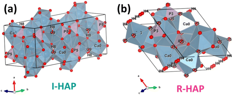 | ||
| Fig. 3 Crystal structure of (a) I-HAp and (b) R-HAp. | ||
3.1.3.1 Scherrer's method (SM). The classic Scherrer method for determining CS is given by the following equation,
 | (17) |
One of the vital factors for this calculation is to correct the peak broadening as mentioned below,
| βc2 = βm2 − βi2 | (18) |
3.1.3.2 Scherrer equation average method (SEAM). Unlike the SM, this method takes all the selected peaks into consideration and uses the FWHM of these peaks for calculating the CS.43 The final CS represents the average of all these calculations. Tables S3 and S4† represents the CS calculation based on SEAM for I-HAp and R-HAp, respectively. Analyzing all the selected peaks with their corresponding FWHM (β) values resulted in an average crystallite size of approximately 120 nm and 115 nm for I-HAp and R-HAp, respectively.
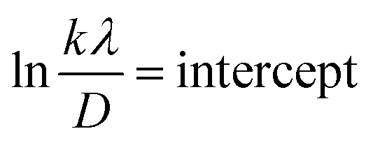
3.1.3.3 Linear straight-line method (LSLM). Introduction of LSLM was done by rearranging the Scherrer equation (eqn (17)) as following,
 | (19) |
Eqn (19) can be compared with the linear straight-line equation, and a plot of cosθ versus 1/β will produce a linear straight line (linear fitting). The slope of the fitted line will be equal to  , from which CS can easily be estimated. Following such, plots for I-HAp and R-HAp were plotted (Fig. 4) and the CS was estimated to be 1626 nm and 10271 nm, respectively.
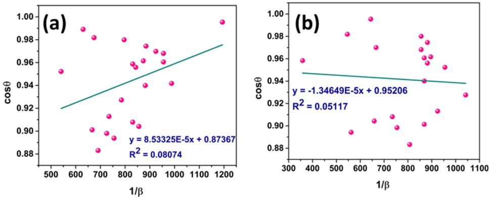 | ||
| Fig. 4 CS estimation by LSLM: (a) I-HAp and (b) R-HAp. | ||
3.1.3.4 Straight line passing the origin method (SLPOM). This method was first proposed by Rabiei et al. in their work41 for CS estimation of HAp prepared from natural sources. This method uses eqn (20) to calculate the slope by forcing the fitted line to pass through the origin. The values of x and y correspond to the values of 1/β and cos
θ, respectively, taken from LSLM (eqn (19)).
 | (20) |
Using this method, slopes for I-HAp and R-HAp was found to be 0.00112262 and 0.001155638, which resulted in CS of 124 nm and 120 nm respectively (slope equals to  ).
).
3.1.3.5 Monshi–Scherrer method (M–SM). In 2012, Monshi et al. implemented adjustments to the Scherrer equation (eqn (17)), presenting a new formula (eqn (21)).44 The Scherrer equation typically yields larger nanocrystalline sizes as inter-atomic layer distance (d) decreases and 2θ values increase, due to the inability to maintain β
cosθ as constant. Additionally, the M–SM offers the benefit of reducing errors, thereby enhancing the accuracy of CS derived from various peaks.
 | (21) |
Fig. 5 represents the plots of lnβ versus ln(1/cosθ) for both I-HAp and R-HAp where linear fitting resulted in the following eqn (22),
 | (22) |
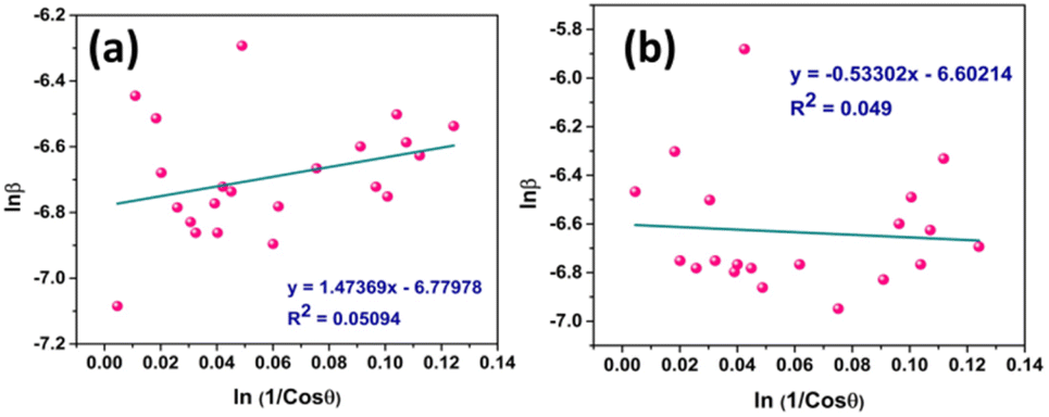 | ||
| Fig. 5 CS estimation by M–SM: (a) I-HAp and (b) R-HAp. | ||
The CS can easily be calculated from eqn (22) and by doing so; CS I-HAp and R-HAp were estimated to be 122 nm and 102 nm respectively.
3.1.3.6 Halder–Wagner method (H–WM). The H–W method was introduced under the premise that peak widening follows a symmetric Voigt function, formed by the convolution of Lorentzian and Gaussian functions.45,46 By assuming a symmetric Voigt function for peak broadening, the Halder–Wagner method aims to provide a more precise estimation of CS, particularly in nanocrystalline materials, compared to traditional methods like the Scherrer equation. Voight function comprising the FWHM of the physical profile is expressed by eqn (23),
| βhkl2 = βL × βhkl + βG2 | (23) |
 | (24) |
 | (25) |
 | (26) |
Putting the values from eqn (25) and (26) into eqn (24) transforms to eqn (27) as follows,
 | (27) |
Plot of 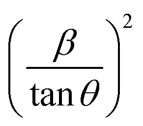 versus
 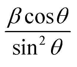 is represented in Fig. 6 where linear fitting of the data values resulted in the slope equal to
  . This was applied for both I-HAp and R-HAp samples and the CS was estimated to be 106 nm and 126 nm respectively.
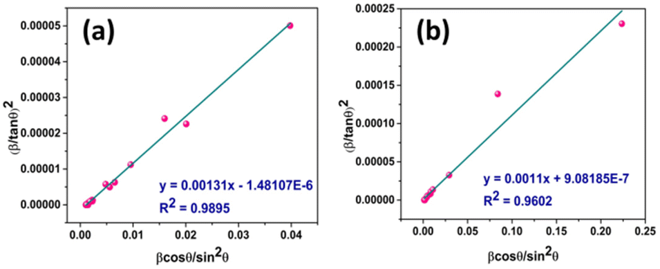 | ||
| Fig. 6 CS estimation by H–WM: (a) I-HAp and (b) R-HAp. | ||
3.1.3.7 Williamson–Hall method (W–HM). The W–H method was utilized to estimate the CS of I-HAp and R-HAp. In contrast to the Scherrer method, the W–H method accounts not only for the impact of CS on XRD peak broadening but also considers the influence of strain-induced XRD peak broadening. Additionally, the W–H model offers a computational approach for estimating both CS and intrinsic strain. This model eliminates the 1/cos
θ dependency by incorporating variation with tanθ in strain considerations.47–49 In a powdered sample, strain results from flaws and distortions in the crystals.41 In light of this, the W–H technique combines the effects of size and strain to describe the total physical line broadening (FWHM) of X-ray diffraction peaks, as shown in eqn (28),| βtotal = βsize + βstrain | (28) |
Strain is a result of crystal distortions and/or defects, and it can be computed using eqn (29).
 | (29) |
Putting the value of strain in eqn (28) and rearranging it by combining with eqn (17) resulted in eqn (30),
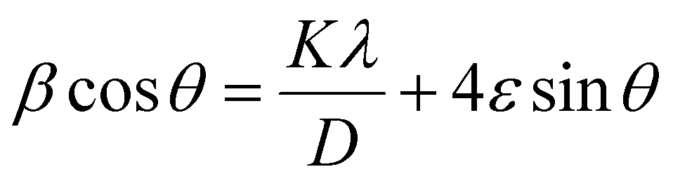 | (30) |
Fig. 7 represents the plots of βcosθ versus 4sinθ for both I-HAp and R-HAp where linear fitting resulted in the following eqn (31),
 | (31) |
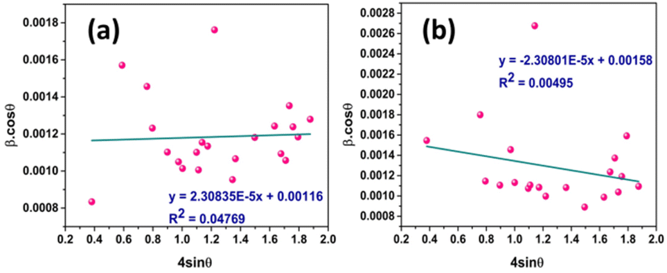 | ||
| Fig. 7 CS estimation by W–HM: (a) I-HAp and (b) R-HAp. | ||
The CS can easily be calculated from eqn (31) and by doing so, CS of I-HAp and R-HAp were estimated to be 120 nm and 88 nm respectively.
3.1.3.8 Size–strain plot method (SSPM). The SSP method gives the data gathered from reflections at high angles less weight. For isotropic broadening, this has a better outcome since XRD data are of lesser quality and peaks overlap at higher angles and higher diffracting. Presumably, the strain profile is represented by the Gaussian function, while the crystallite size is represented by the Lorentzian function. Additionally, eqn (32) states the overall broadening of this approach, where βL and βG represent the peak broadening by the simultaneous application of Lorentz and Gaussian functions.41
| βhkl = βL + βG | (32) |
The equation associated with SSPM is given by eqn (33),
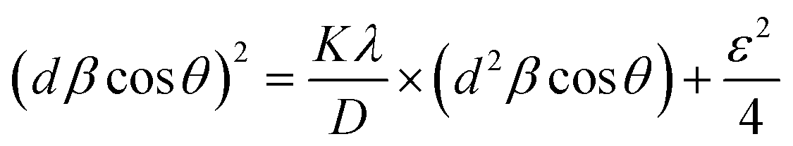 | (33) |
The inter-atomic layer distance (d) for I-HAp and R-HAp was taken from eqn (1) and (2) respectively.
Fig. 8 represents the plots of dβcosθ versus d2βcosθ for both I-HAp and R-HAp where linear fitting resulted in the following eqn (34),
 | (34) |
 | ||
| Fig. 8 CS estimation by SSPM: (a) I-HAp and (b) R-HAp. | ||
The CS can easily be calculated from eqn (34) and by doing so, CS I-HAp and R-HAp was estimated to be 123 nm and 87 nm respectively.
Table 3 summarizes the calculated crystallite size of I-HAp and R-HAp samples following different methods. Methods such as Scherrer's method (SM), Scherrer equation average method (SEAM), and straight line passing the origin method (SLPOM) don't require the linear fitting of plots to calculate the CS and can be estimated directly from the respective equations. According to these three methods, the estimated CS of I-HAp ranges between 120 and 135 nm and for R-HAp it is 115–129 nm. The CS of R-HAp estimated through these three methods is slightly smaller than I-HAp.
| Method | Abbreviation | Calculated crystallite size (nm) | |||
|---|---|---|---|---|---|
| I-HAp | R2 | R-HAp | R2 | ||
| Scherrer's method | SM | 135 | — | 129 | — |
| Scherrer equation average method | SEAM | 120 | — | 115 | — |
| Linear straight-line method | LSLM | 1626 | 0.0807 | 10271 |
0.0512 |
| Straight line passing the origin | SLPOM | 124 | — | 120 | — |
| Monshi–Scherrer method | M–SM | 122 | 0.0509 | 102 | 0.0490 |
| Halder–Wagner method | H–WM | 106 | 0.9895 | 126 | 0.9602 |
| Williamson–Hall method | W–HM | 120 | 0.0477 | 88 | 0.0049 |
| Size–strain plot method | SSPM | 123 | 0.8580 | 87 | 0.9698 |
When choosing the best fitted data based on the highest R2 value, the Halder–Wagner method (H–WM) is the best suited for estimating the CS of I-HAp (R2 = 0.9895) which resulted in 106 nm. For R-HAp, the best suited method was size–strain plot method (SSPM) which resulted in CS of 87 nm (R2 = 0.9698). The CS of R-HAp is also smaller in this case.
3.2 Morphological analysis
Morphological analysis of the prepared I-HAp and R-HAp samples was carried out in terms of FESEM and TEM, which is presented in Fig. 9. | ||
| Fig. 9 I-HAp: (a) and (b) FESEM images and (c) corresponding size distribution histogram, (d) and (e) TEM images and (f) corresponding size distribution histogram; R-HAp: (g) and (h) FESEM images and (i) corresponding size distribution histogram, (j) and (k) TEM images and (l) corresponding size distribution histogram. | ||
The FESEM images of I-HAp at two different magnifications (Fig. 9a and b) clearly indicate the formation of large particles (greater than 100 nm) that were thermally treated at 1000 °C for 3 hours. The particles are bulky in nature with multiple sides and sharp edges. Both aggregation and agglomeration are present in these particles. The size of the particles was measured using ImageJ software, and the procedure can be found elsewhere.35 The average size of I-HAp particles was found to be 703 ± 175 nm (n = 68). Particles of R-HAp samples are comparatively smaller in size (Fig. 9g and h). The average size of R-HAp particles was 565 ± 195 nm (n = 890).
The morphology of R-HAp particles is similar to I-HAp particles; except for the fact that the surface of I-HAp particles is smoother. Rough edges and fragmentation were more frequent in the surfaces of R-HAp particles. The presence of aggregation and agglomeration was also confirmed through the TEM images for both of the samples (Fig. 9d and j). This caused the distinction of particles very hard, and only a few particles could be selected for the size calculation (Fig. 9f and l). Fragmentation of particles can also be found in the TEM images, and they weren't considered as particles during the size calculation. Lattice fringes were visible at higher magnification, and the interplanar distances (d-spacing) for both samples were measured. For I-HAp, d-spacing was measured to be 0.333 ± 0.034 nm which indicates the (002) plane, as observed through the XRD analysis. Similarly for R-HAp, d-spacing was 0.283 ± 0.032 nm, which was very much closer to the d-spacing value of (211) plane (0.281 nm). The measured average size of R-HAp particles based on the TEM image was smaller than that of the I-HAp, which is confluent with the FESEM image-based size estimation.
3.3 XPS analysis
The surface elemental composition of the prepared HAp samples from Tenualosa ilisha and Labeo rohita FS was evaluated by XPS analysis and presented in Fig. 10. The survey scan of both of the HAp samples (Fig. 10a) produced a similar spectrum, and the elements of HAp (Ca, P, and O) were detected. Additionally, C, Na, and Mg were also detected. The presence of C can be attributed to the hydrocarbons, which are existent as impurities and widely denoted as “adventitious carbon”.14 The presence of Na and Mg in the HAp samples is likely due to the natural composition of the FS. As mentioned in previous literature,50,51 FS can contain trace elements such as Na+ and Mg2+ that substitute into the calcium positions of the HAp structure. Apart from that, the use of NaOH during the alkali treatment process is a potential source of Na incorporation into the HAp samples. The narrow scan spectra were deconvoluted to analyze the chemical states of these elements. For Ca 2p (Fig. 10b), the deconvoluted spectra showed two peaks for both HAp samples, corresponding to the Ca2+ ions in the HAp structure. For I-HAp, peaks at 350.78 eV and 347.38 eV confined within the envelope can be attributed to the Ca 2p1/2 and Ca 2p3/2 with the doublet separation of 3.40 eV. | ||
| Fig. 10 XPS analysis of the prepared HAp samples (I-HAp and R-HAp): (a) survey spectra; high resolution narrow scan spectra of (b) Ca 2p; (c) P 2p; (d) O 1s; (e) C 1s; (f) Na 1s and (g) Mg 1s. | ||
Similarly, R-HAp produced these peaks at 350.88 eV and 347.18 eV and the doublet separation was 3.70 eV. The differences in the doublet separation indicate differences in the crystal structure and chemical environment between the two HAp samples. A larger doublet separation suggests a more crystalline structure of the R-HAp sample, which is also supported by the XRD report. The P 2p narrow scan spectra (Fig. 10c) also produced two peaks upon deconvolution due to the spin–orbit splitting, indicating the presence of phosphate groups in the HAp lattice. For I-HAp, peaks at 133.88 eV and 133.08 eV correspond to P 2p1/2 and P 2p3/2, whereas peaks at 134.08 eV and 132.98 eV correspond to P 2p1/2 and P 2p3/2 respectively. Similarly, as the Ca 2p doublet separation, R-HAp has a higher P 2p doublet separation (1.1 eV) compared to I-HAp (0.8), indicating a more crystalline nature. The O 1 s spectra (Fig. 10d) showed two peaks for both I-HAp (at 531.68 eV and 532.78 eV) and R-HAp (at 531.18 eV and 532.78 eV), which can be attributed to the lattice oxygen and surface hydroxyl groups, respectively.
For both I-HAp and R-HAp, the C 1s spectra (Fig. 10e) showed four peaks, suggesting the presence of various carbon species, such as carbonate and organic contaminants, on the HAp surface. Single peaks were seen in the Na 1s (Fig. 10f) and Mg 1s (Fig. 10g) spectra for both I-HAp (1071.88 eV and 1304.18 eV, respectively) and R-HAp (1071.98 eV and 1304.38 eV, respectively), confirming the incorporation of Na+ and Mg2+ ions into the HAp structure.
3.4 DLS size and zeta potential analysis
Further analysis into the particle size of the prepared HAp samples was done by DLS analysis, along with the surface charge measurements in terms of zeta potential analysis. Fig. 11 illustrates the plots of DLS particle size and zeta potential measurements. | ||
| Fig. 11 DLS particle size and zeta potential measurements of I-HAp and R-HAp: (a) correlograms; (b) intensity-based, (c) volume-based, and (d) number-based size distribution; (e) zeta potential measurements; and (f) plot of phase analysis light scattering (PALS-phase plot). Measurements were carried out at a sample concentration of 0.1 mg mL−1, pH was solution natural pH at 25 ± 1 °C. | ||
The correlogram (Fig. 11a) for both I-HAp and R-HAp samples indicates a larger size distribution (greater than 100 nm). The value of the Y-intercept of R-HAp was lower than that of I-HAp. This indicates a weaker initial correlation, possibly due to a higher level of noise in the measurement. The Y-intercept value less than 1 for both samples indicate the presence of multiple scattering, which occurs when a photon of light interacts with multiple particles before reaching the detector, and this might happen several times before the light is finally reached. Such phenomena might have occurred due to higher sample concentrations.52 The DLS hydrodynamic diameter (herein termed as DLS particle size) was presented in terms of intensity, volume, and number percentages (Fig. 11b–d) to get an overall picture of the size distribution. The intensity percentage-based size distribution produced two peaks of distribution, one at lower size with lower intensity and the other one with higher size and intensity, for both of the samples. This indicates the presence of two different sizes. The z-average sizes of I-HAp and R-HAp were found to be 687 and 617 nm respectively, based on the intensity percentage plot. This finding is consistent with the size measurements based on the FESEM images, where I-HAp had larger particles. The volume percentage-based size distribution plot was consistent with the intensity percentage plot; however, the number percentage-based size distribution plot produced the scenario where lower sizes had the highest intensity. The average sizes of these particles were 108 and 146 nm respectively, and the presence of such particles might be from the fragmentation of the larger particles as seen in the FESEM images. The polydispersity index (PDI) values were 0.6303 for I-HAp and 0.456 for R-HAp, indicating a relatively broad size distribution.
The zeta potential analysis of I-HAp produced two peaks (−38.73 mV and +28.38 mV) while for R-HAp, it produced three peaks (−48.32 mV, −29.14 mV and +60.34 mV). The presence of multiple peaks in the zeta potential plot (Fig. 11e), with both positive and negative charges for both of the samples, indicates their polydisperse nature. Such polydispersity depicts the variation in particle size and surface charge distributions. The higher number of peaks and greater zeta deviation in R-HAp compared to I-HAp suggests that the HAp derived from Labeo rohita scales has a more heterogeneous surface charge distribution. This could be attributed to differences in the composition and structure of the scales between the two fish species.53,54 The quality factor, which represents the ratio of the mean zeta potential to the zeta deviation, is higher for R-HAp (3.003) compared to I-HAp (1.555). A higher quality factor indicates better stability of the HAp particles in suspension due to stronger repulsive forces between the particles, which prevents agglomeration.55 Plots of phase analysis light scattering (PALS-phase plot) for I-HAp and R-HAp samples show (Fig. 11f) the change in phase difference over time between two detection points that receive light scattered from the particles. The plots with a saw-tooth like pattern at a lower time-frame indicate the goodness of the data for electrophoretic mobility and zeta potential.
3.5 Elemental composition and mapping
Elemental composition, along with the mapping of these elements for the I-HAp and R-HAp samples, is presented in Fig. 12 respectively. The relative amounts of each element are shown in the spectrum (Fig. 12a and g), while the mass and weight percentages provide quantitative details about the composition. Calcium (Ca Ka and Ca Kb), phosphorus (P Ka), and oxygen (O Ka) were the primary elements detected and quantified for both the samples. Apart from these elements, Na Ka, Mg Ka and C Ka were also detected. | ||
| Fig. 12 Elemental analysis of the prepared HAp samples: (a) EDX spectrum and (b)–(f) corresponding mapping of elements of I-HAp; (g) EDX spectrum and (h)–(l) corresponding mapping of elements of R-HAp. | ||
As mentioned in the XPS analysis, the presence of Na and Mg in the HAp samples is probably because of the natural makeup of FS. These elements can take the place of Ca in the HAp structure. Also, using NaOH during the alkali treatment process can bring more Na into the HAp samples. The presence of C could be due to the atmospheric CO2 or the carbon tape that was used as a substrate for the samples. The Ca/P ratio of I-HAp and R-HAp samples was 1.42 and 1.41, respectively (based on atom%). Notably, the Ca/P ratios in both samples were very similar, and both fell below the theoretical value of 1.67. In the HAp crystal structure, some Ca positions might be replaced by other elements like Mg or Na that were detected in the EDX analysis. These elements have lower atomic weights than Ca, affecting the overall Ca/P ratio.56
The elemental mapping of I-HAp and R-HAp samples revealed distinct patterns of elemental distribution of HAp. For I-HAp (Fig. 12b–f), calcium and phosphorus were strongly correlated, while O was evenly dispersed. Na and Mg were present in smaller amounts and were not as spatially correlated groups. In contrast, R-HAp showed (Fig. 12h–l) a slightly more heterogeneous O distribution and higher amounts of Na and Mg. Amount of C was also higher, possibly due to more organic impurities. These differences may be related to variations in fish scales, as the processing conditions were the same.
3.6 Functional group analysis by FTIR and Raman spectroscopy
Functional group analysis of the prepared I-HAp and R-HAp samples was carried out by the aid of FTIR and Raman spectroscopic analysis. The FTIR spectra of the HAp samples are presented in Fig. 13a. FTIR spectra of both of the samples are analogous to the typical HAp spectrum, with the presence of PO43− , OH− and CO32− groups. The characteristic bands of PO43− group, symmetric and asymmetric bending (ν2 and ν4), and symmetric and asymmetric stretching (ν1 and ν3) were present for both I-HAp and R-HAp samples. The presence of bands for structural OH− group was noticed at around 630 cm−1 and 3568 cm−1 for both of the samples. The intensity of these bands was very low for the R-HAp sample, with the later one being the lowest in intensity. The presence of CO32− group was also detected for both samples, at two different positions.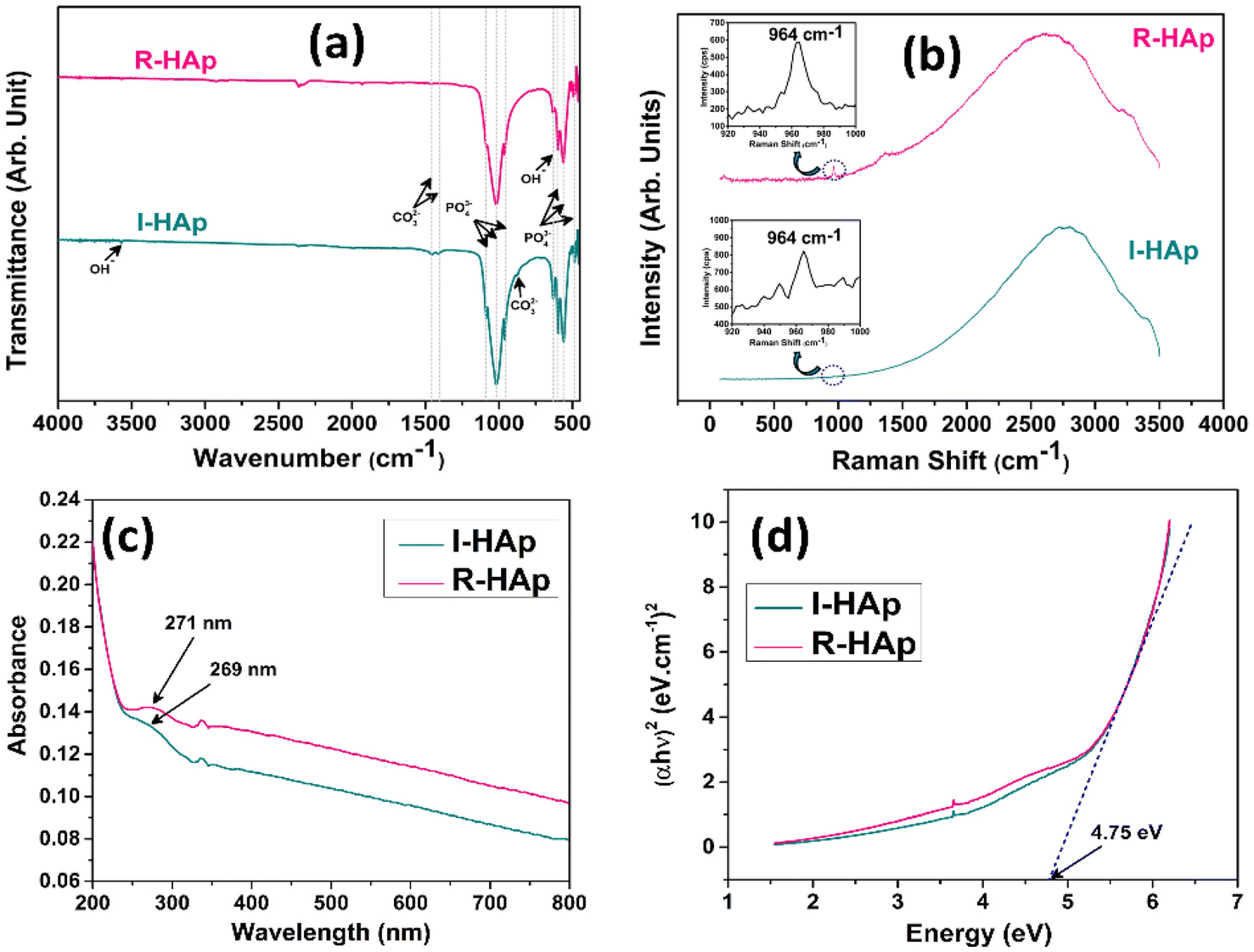 | ||
| Fig. 13 (a) FTIR analysis; (b) Raman spectroscopic analysis; (c) UV-visible spectra and (d) Tauc plot for band gap measurements of I-HAp and R-HAp sample. | ||
For I-HAp sample, the band position at around 879, 1413 and 1458 cm−1 correspond to the CO32− group. For R-HAp, band position of CO32− group was observed only at 1458 cm−1. The presence of this CO32− group at these aforementioned positions can be attributed to the B-type substitution, which is the substitution of PO43− group by the CO32− group. The incorporation of this B-type CO32− into the HAp lattice occurs through a process called carbonate substitution.57 There are quite a few studies that report the effect of B-type substitution on the HAp lattice. For instance, the stability and solubility of HAp can be affected by this substitution which ultimately influences the bioactivity in bone regeneration applications. In addition, such substitution of carbonate group might enhance the resorption rate of HAp implants in the body.58 All the FTIR bands that have been detected and their assignments are summarized in Table 4.
| Vibrational frequency (cm−1) | Corresponding assignments | Marking | |
|---|---|---|---|
| I-HAp | R-HAp | ||
| 3568 | 3568 | Structural OH− | ν |
| 1458 | 1458 | B-type CO32− | ν3 |
| 1413 | — | B-type CO32− | ν3 |
| 1085 | 1072 | Asymmetric stretching of PO43− | ν3 |
| 1018 | 1020 | Asymmetric stretching of PO43− | ν3 |
| 960 | 960 | Symmetric stretching of PO43− | ν1 |
| 879 | — | B-type CO32− | δ |
| 630 | 632 | Structural OH− | ν |
| 597 | 599 | Asymmetric bending of PO43− | ν4 |
| 559 | 559 | Asymmetric bending of PO43− | ν4 |
| 486 | 495 | Symmetric bending of PO43− | ν2 |
The Raman spectroscopic analysis of the samples was carried out within the Raman shift range of 50–3500 cm−1 which produced broad shaped peak for both of the samples (Fig. 13b). Peak at 964 cm−1 (shown in the inset plots) confirms the presence of PO43− group within the samples. This peak corresponds to the characteristic symmetrical stretching vibration of these groups, indicating the formation of an apatite-like structure.59
3.7 UV-visible spectroscopic analysis
The UV-visible spectra of the I-HAp and R-HAp samples, dispersed in DI at solution pH is shown in Fig. 13c. Both of the spectrum has similar pattern with an absorption at nearly similar position. For I-HAp, absorption peak is observed at 269 nm whereas R-HAp shows peak at 271 nm. For pure HAp, the peak of absorption is typically observed in the UV region of 200–340 nm. Ain et al. reported an absorption peak of HAp at 274 nm with a peak band at 247 nm.60 The most likely reason behind this absorption peak is due to the scattering of irradiated light by the colloidal HAp particles.61 The TEM measurement revealed a portion of particles that are in the nanometer scale and these nanoparticles might contribute to this scattering. The small UV-visible absorption peak observed for both HAp samples is attributed to the limited quantity of nanometer-scale particles.The optical bandgap of the prepared HAp samples was calculated using the UV-visible data through the Tauc plot method which is governed by the following equation,62
| αhν = A(hν − Eg)n | (35) |
3.8 Biocompatibility study in terms of cell viability and hemocompatibility study
The successful implementation of a biomaterial mainly depends on its safety while it comes in contact with the physiological environment. Keeping this in mind, the biocompatibility of the prepared I-HAp and R-HAp samples were examined in terms of cell viability and hemolysis study.Fig. 14a–g represents the results of cell viability of the prepared HAp samples on vero cell lines. The assessment reveals that, both I-HAp and R-HAp samples show no sign of cytotoxicity as the cell viability was above 95% in both cases. For a material to be termed as cytocompatible, the cell viability should be more than 70%.63 Based on this definition, the Tenualosa ilisha and Labeo rohita derived HAp samples are cytocompatible in nature.
 | ||
| Fig. 14 Cell viability study of the prepared HAp samples from Tenualosa ilisha and Labeo rohita fish scale: microscopic images of vero cells cultured with (a) 100 and (b) 200 μg mL−1 of I-HAp; (c) 100 and (d) 200 μg mL−1 of R-HAp; (e) negative control; (f) positive control; (g) results and summary of cell viability study (the amount of sample and incubation time was 25 μL and 48 h respectively); (h) hemolysis study of the HAp samples (for 100 μg mL−1 sample concentration each). | ||
Fig. 14h represents the hemocompatibility assessment results of the HAp samples. This study is also an important examination of biomaterials that come in close contact with blood. When a material causes lysis of red blood cell, it begets the release of hemoglobin. By measuring the amount of hemoglobin through UV-visible spectrophotometer, percentage of hemolysis is measured. Both I-HAp and R-HAp samples showed around 1% hemolysis, depicting their safety as a biomaterial.1,13,64
3.9 Bio-activity analysis
One way of studying the bio-active nature of biomaterials, in this case HAp, is the confirmation of apatite layer formation through an electron microscope after immersing in SBF solution for a certain time.65,66 The prepared I-HAp and R-HAp samples were examined with FESEM after immersing them in SBF solution for 3 weeks at 37 °C. The captured images are presented in Fig. 15 where the formation of apatite crystals and layers over the HAp particles is evident. The obtained images reveal a rare occurrence of highly porous, hemispherical globule-like structures coated with an interlinked apatite layer. Identical structures were also reported by Chavan et al. which also denoted the structures as interlinked apatite layers.67 This observation indicates the formation of a bone-like apatite layer on the surface of the fish scale-derived HAp samples, suggesting their potential bioactivity and ability to promote bone cell growth and mineralization. The formation of an apatite layer on the surface of HAp materials when immersed in SBF is considered a good indicator of their in vivo bone-bonding ability and bioactivity.68 The apatite layer formation is facilitated by the release of calcium and phosphate ions from the HAp material, which leads to the nucleation and growth of a bone-like apatite layer on the surface.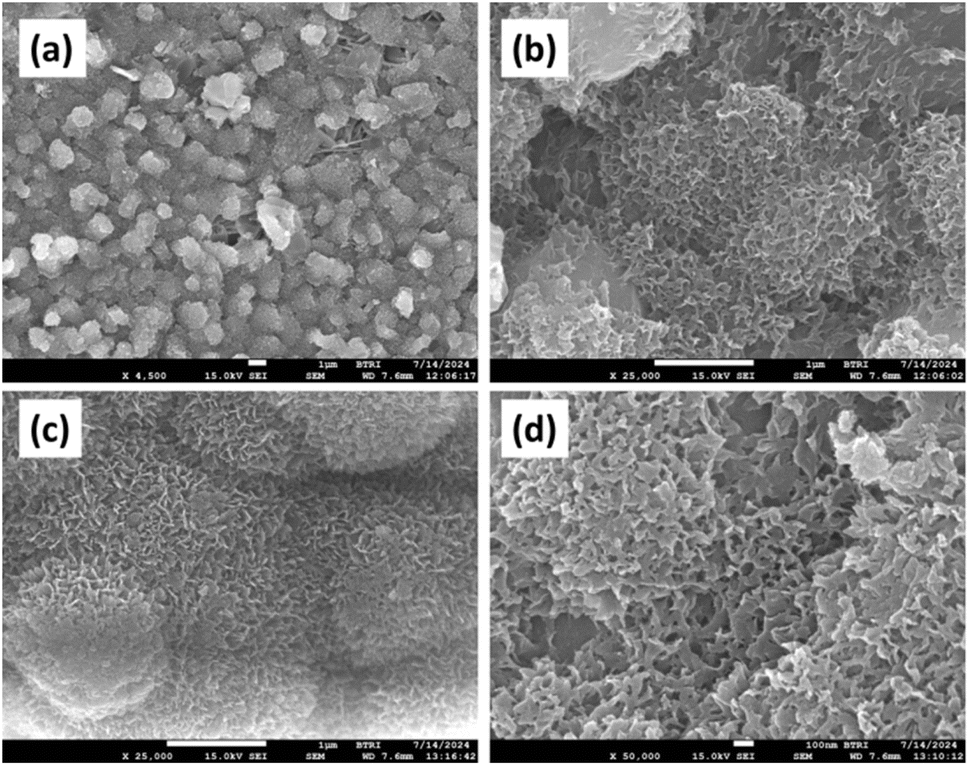 | ||
| Fig. 15 Bioactivity assessment of the HAp samples after 3 weeks of immersion in SBF solution at 37 °C: (a) and (b) I-HAp and (c) and (d) R-HAp. | ||
Interestingly, in our previous study following a similar methodology, the 3 weeks of SBF immersed HAp samples (prepared from waste chicken eggshells) resulted in supersaturation of particles rather than forming highly porous apatite structures.1,13
4. Conclusion
This study compared two HAp samples derived from the scales of Tenualosa ilisha and Labeo rohita fish in terms of their crystallographic characteristics, functional groups, morphology, elemental composition, particle size, and bioactivity. XRD analysis revealed that HAp from Tenualosa ilisha scales predominantly grew along the (002) plane, while that from Labeo rohita scales favored the (211) plane. Crystallite size calculations using different model equations indicated mostly the formation of micro-sized HAp crystallites after calcination at 1000 °C. The Tenualosa ilisha-derived HAp (I-HAp) exhibited larger crystallite and particle sizes than the Labeo rohita-derived HAp (R-HAp), as determined by FESEM, TEM, and DLS. FTIR, Raman, FESEM, TEM, EDX, DLS, and zeta potential analyses indicated a high degree of similarity between the prepared samples, including their bioactive nature. This research framework will aid in selective preparation of HAp with monoclinic crystal structure and bio-competency from waste fish scales of Tenualosa ilisha.Ethical statement
This study was conducted in accordance with IGCRT guidelines and received ethical clearance from the BCSIR Ethics Committee (ref.: IGCRT/R&D research/2022-2024/01; date: 04.10.2022) prior to the commencement of the hemocompatibility study. Informed consent was obtained from all human subjects involved in the study.Data availability
The data used for this research is provided in the main article and its accompanying ESI.†Author contributions
Mashrafi Bin Mobarak: methodology, investigation, data curation, writing – original draft. Fariha Chowdhury: investigation, data curation. Samina Ahmed: supervision, writing – review and editing.Conflicts of interest
There is no conflict to declare.Acknowledgements
This study was carried out under the approved project of Bangladesh Council of Scientific and Industrial Research (BCSIR) (R&D reference no. 39.02.0000.011.14.169.2023/877; date: 17/09/2023). We express our heartfelt gratitude to Md. Sahadat Hossain, Sabrina Mostafa, Dr Umme Sarmeen Akhtar and Nazmul Islam Tanvir for helping out with the XRD, TEM, XPS and Raman analysis, respectively.References
- M. B. Mobarak, M. N. Islam, F. Chowdhury, M. N. Uddin, M. S. Hossain, M. Mahmud, U. S. Akhtar, N. I. Tanvir, A. M. Rahman and S. Ahmed, RSC Adv., 2023, 13, 36209–36222 RSC.
- S. Sultana, M. S. Hossain, M. Mahmud, M. B. Mobarak, M. H. Kabir, N. Sharmin and S. Ahmed, RSC Adv., 2021, 11, 3686–3694 RSC.
- G. Ma and X. Y. Liu, Cryst. Growth Des., 2009, 9, 2991–2994 CrossRef CAS.
- M. B. Mobarak, M. S. Hossain, Z. Yeasmin, M. Mahmud, M. M. Rahman, S. Sultana, S. M. Masum and S. Ahmed, J. Mol. Struct., 2022, 1252, 132142 CrossRef.
- M. S. Hossain, M. Mahmud, S. Sultana, M. Bin Mobarak, M. S. Islam and S. Ahmed, R. Soc. Open Sci., 2021, 8, 210684 CrossRef PubMed.
- H. Shi, Z. Zhou, W. Li, Y. Fan, Z. Li and J. Wei, Crystals, 2021, 11, 149 CrossRef CAS.
- H. Liu, W. Jiang and A. Malshe, JOM, 2009, 61, 67–69 CAS.
- S. Lara-Ochoa, W. Ortega-Lara and C. E. Guerrero-Beltrán, Pharmaceutics, 2021, 13, 1642 CrossRef CAS PubMed.
- S. Allegrini Jr, E. Rumpel, E. Kauschke, J. Fanghänel and B. König Jr, Ann. Anat., 2006, 188, 143–151 CrossRef PubMed.
- D.-E. Radulescu, O. R. Vasile, E. Andronescu and A. Ficai, Int. J. Mol. Sci., 2023, 24, 13157 CrossRef CAS PubMed.
- R. Verma, S. R. Mishra, V. Gadore and M. Ahmaruzzaman, Adv. Colloid Interface Sci., 2023, 315, 102890 CrossRef CAS PubMed.
- M. Hossain, M. Mahmud, M. B. Mobarak and S. Ahmed, Chem. Pap., 2022, 76, 1593–1605 CrossRef CAS.
- M. B. Mobarak, M. N. Uddin, F. Chowdhury, M. S. Hossain, M. Mahmud, S. Sarkar, N. I. Tanvir and S. Ahmed, J. Mol. Struct., 2024, 1301, 137321 CrossRef.
- M. B. Mobarak, N. S. Pinky, F. Chowdhury, M. S. Hossain, M. Mahmud, M. S. Quddus, S. A. Jahan and S. Ahmed, J. Saudi Chem. Soc., 2023, 101690 CrossRef.
- S. H. Daryan, A. Khavandi and J. Javadpour, Solid State Sci., 2020, 106, 106301 CrossRef CAS.
- J. Jiang, Y. Long, X. Hu, J. Hu, M. Zhu and S. Zhou, J. Solid State Chem., 2020, 289, 121491 CrossRef CAS.
- M. K. Yadav, R. H. Shukla and K. G. Prashanth, Mater. Today: Proc., 2023 DOI:10.1016/j.matpr.2023.04.669.
- D. Qin, S. Bi, X. You, M. Wang, X. Cong, C. Yuan, M. Yu, X. Cheng and X.-G. Chen, Chem. Eng. J., 2022, 428, 131102 CrossRef CAS.
- T. Eknapakul, S. Kuimalee, W. Sailuam, S. Daengsakul, N. Tanapongpisit, P. Laohana, W. Saenrang, A. Bootchanont, A. Khamkongkaeo and R. Yimnirun, RSC Adv., 2024, 14, 4614–4622 RSC.
- P. Deb and A. B. Deoghare, Bull. Mater. Sci., 2019, 42, 3 CrossRef.
- S. Hamzah, N. I. Yatim, M. Alias, A. Ali, N. Rasit and A. Abuhabib, Indones. J. Chem., 2019, 19, 1019–1030 CrossRef CAS.
- Department of Fisheries, https://fisheries.portal.gov.bd/site/view/annual_reports, accessed July 31, 2024.
- S. Network, Fish scales, https://seafoodnetworkbd.com/fish-scales-transforming-waste-into-export-wealth-for-bangladesh, accessed July 31, 2024.
- M. A. Rouf, M. R. Golder, N. A. Kana, S. Debnath, M. M. Rahman, R. T. Mathew and Y. N. Alrashada, Advances in Animal and Veterinary Sciences, 2021, 9, 2194–2200 Search PubMed.
- A. R. Sunny, M. N. Hassan, M. Mahashin and M. Nahiduzzaman, Journal of Entomology and Zoology Studies, 2017, 5, 2099–2105 CrossRef.
- M. S. Hossain, S. M. Sharifuzzaman, M. A. Rouf, R. S. Pomeroy, M. D. Hossain, S. R. Chowdhury and S. AftabUddin, Fish and Fisheries, 2019, 20, 44–65 CrossRef.
- S. Dutta and S. Hazra, Indian J. Geo-Mar. Sci., 2017, 46(08), 1503–1510 Search PubMed.
- S. Mondal, S. Mahata, S. Kundu and B. Mondal, Adv. Appl. Ceram., 2010, 109, 234–239 CrossRef CAS.
- M. B. Mobarak, F. Chowdhury, M. N. Uddin, M. S. Hossain, U. Akhtar, N. I. Tanvir, M. A. A. Shaikh and S. Ahmed, Mater. Adv., 2024, 5, 9716–9730 RSC.
- S. Z.-H. Ejaz, S. Iqbal, S. Shahida, S. M. Husnain and M. Saifullah, New J. Chem., 2023, 47, 443–452 RSC.
- A. Yücel, S. Sezer, E. Birhanlı, T. Ekinci, E. Yalman and T. Depci, Ceram. Int., 2021, 47, 626–633 CrossRef.
- T. V. Kolekar, N. D. Thorat, H. M. Yadav, V. T. Magalad, M. A. Shinde, S. S. Bandgar, J. H. Kim and G. L. Agawane, Ceram. Int., 2016, 42, 5304–5311 CrossRef CAS.
- J. C. C. Abrantes, A. Kaushal, S. Pina, N. Döbelin, M. Bohner and J. M. F. Ferreira, J. Eur. Ceram. Soc., 2016, 36, 817–827 CrossRef.
- T. Saha, M. B. Mobarak, M. N. Uddin, M. S. Quddus, M. R. Naim and N. S. Pinky, Mater. Chem. Phys., 2023, 305, 127979 CrossRef CAS.
- M. Bin Mobarak, M. S. Hossain, F. Chowdhury and S. Ahmed, Arabian J. Chem., 2022, 15, 104117 CrossRef CAS.
- M. S. Hossain, S. Sarkar, S. Tarannum, S. M. Tuntun, M. Mahmud, M. B. Mobarak and S. Ahmed, J. Saudi Chem. Soc., 2023, 27, 101769 CrossRef.
- M. Sharma, R. Nagar, V. K. Meena and S. Singh, RSC Adv., 2019, 9, 11170–11178 RSC.
- K. Momma and F. Izumi, J. Appl. Crystallogr., 2011, 44, 1272–1276 CrossRef CAS.
- A. Bishnoi, S. Kumar and N. Joshi, in Microscopy methods in nanomaterials characterization, Elsevier, 2017, pp. 313–337 Search PubMed.
- V. Uvarov and I. Popov, Mater. Charact., 2007, 58, 883–891 CrossRef CAS.
- M. Rabiei, A. Palevicius, A. Monshi, S. Nasiri, A. Vilkauskas and G. Janusas, Nanomaterials, 2020, 10, 1627 CrossRef CAS PubMed.
- A. M. Castillo-Paz, S. M. Londoño-Restrepo, L. Tirado-Mejía, M. A. Mondragón and M. E. Rodríguez-García, Prog. Nat. Sci.: Mater. Int., 2020, 30, 494–501 CrossRef CAS.
- M. S. Hossain, M. S. Hossain, S. Ahmed and M. B. Mobarak, RSC Adv., 2024, 14, 38560–38577 RSC.
- A. Monshi, M. R. Foroughi and M. R. Monshi, World J. Nano Sci. Eng., 2012, 2, 154–160 CrossRef.
- N. C. Halder and C. N. J. Wagner, Acta Crystallogr., 1966, 20, 312–313 CrossRef CAS.
- Y. Canchanya-Huaman, A. F. Mayta-Armas, J. Pomalaya-Velasco, Y. Bendezú-Roca, J. A. Guerra and J. A. Ramos-Guivar, Nanomaterials, 2021, 11, 2311 CrossRef CAS PubMed.
- A. K. Zak, W. A. Majid, M. E. Abrishami and R. Yousefi, Solid State Sci., 2011, 13, 251–256 CrossRef.
- B. E. Warren and B. L. Averbach, J. Appl. Phys., 1952, 23, 497 CrossRef CAS.
- D. Nath, F. Singh and R. Das, Mater. Chem. Phys., 2020, 239, 122021 CrossRef CAS.
- L. M. Cursaru, M. Iota, R. M. Piticescu, D. Tarnita, S. V. Savu, I. D. Savu, G. Dumitrescu, D. Popescu, R.-G. Hertzog and M. Calin, Materials, 2022, 15, 5091 CrossRef CAS PubMed.
- W. Suo-Lian, K. Huai-Bin and L. Dong-Jiao, J. Food Sci. Eng., 2017, 7, 2159–5828 Search PubMed.
- F. Babick, in Characterization of Nanoparticles, Elsevier, 2020, pp. 137–172 Search PubMed.
- S. Mondal, A. Mondal, N. Mandal, B. Mondal, S. S. Mukhopadhyay, A. Dey and S. Singh, Bioprocess Biosyst. Eng., 2014, 37, 1233–1240 CrossRef CAS PubMed.
- P. Deb, E. Barua, S. D. Lala and A. B. Deoghare, Mater. Today: Proc., 2019, 15, 277–283 CAS.
- Intermediate topics in electrophoretic mobility data analysis, https://www.malvernpanalytical.com.cn/learn/knowledge-center/technical-notes/tn101104assessingzetapotentialmeasuremen, accessed July 7, 2024.
- I. Cacciotti, in Handbook of bioceramics and biocomposites, Springer International Publishing, Cham, Switzerland, 2016, vol. 46, pp. 145–211 Search PubMed.
- O. F. Yasar, W.-C. Liao, R. Mathew, Y. Yu, B. Stevensson, Y. Liu, Z. Shen and M. Edén, J. Phys. Chem. C, 2021, 125, 10572–10592 CrossRef CAS.
- R. Yotsova and S. Peev, Pharmaceutics, 2024, 16, 291 CrossRef CAS PubMed.
- U. Anjaneyulu, D. K. Pattanayak and U. Vijayalakshmi, Mater. Manuf. Processes, 2016, 31, 206–216 CrossRef CAS.
- Q. Ain, H. Munir, F. Jelani, F. Anjum and M. Bilal, Mater. Res. Express, 2020, 6, 125426 CrossRef.
- W.-G. Yang, J.-H. Ha, S.-G. Kim and W.-S. Chae, J. Anal. Sci. Technol., 2016, 7, 9 CrossRef.
- F. Chowdhury, M. B. Mobarak, M. Hakim, M. N. Uddin, M. S. Hossain, U. S. Akhter, D. Islam, S. Ahmed and H. Das, New J. Chem., 2024, 48, 17038–17051 RSC.
- I. O. for Standardization, 2009.
- M. S. Hossain, M. A. A. Shaikh, S. A. Jahan, M. Mahmud, M. B. Mobarak, M. S. Rahaman, M. N. Uddin and S. Ahmed, RSC Adv., 2023, 13, 9654–9664 RSC.
- T. Kokubo and H. Takadama, Biomaterials, 2006, 27, 2907–2915 CrossRef CAS PubMed.
- T. Kokubo and H. Takadama, in Handbook of Biomineralization, ed. E. Bäuerlein, Wiley, 1st edn, 2007, pp. 97–109 Search PubMed.
- P. N. Chavan, M. M. Bahir, R. U. Mene, M. P. Mahabole and R. S. Khairnar, Mater. Sci. Eng., B, 2010, 168, 224–230 CrossRef CAS.
- F. Baino and S. Yamaguchi, Biomimetics, 2020, 5, 57 CrossRef CAS PubMed.
Footnote |
| † Electronic supplementary information (ESI) available. See DOI: https://doi.org/10.1039/d4ra06662f |
| This journal is © The Royal Society of Chemistry 2024 |