Active nematic coherence probed under spatial patterns of distributed activity

Abstract

A photoresponsive variant of the paradigmatic active nematic fluid made of microtubules and powered by kinesin motors is studied in a conventional two-dimensional interface under blue-light illumination. This advantageously permits the system's performance to be assessed under conditions of spatially distributed activity. Both turbulent and flow aligning conditions are separately analyzed. Under uniform illuminating conditions, active flows get enhanced, in accordance with previous observations. In contrast, patterning the activity appears to disturb the effective activity measured in terms of the vorticity of the elicited flows. We interpret this result as alternative evidence of the important role played by the active length scale in setting not only the textural and flow characteristics of the active nematic but also, most importantly, the range of material integrity. Our research continues to explore perspectives that should pave the way for an effective control of such an admirable material.

---

1. Introduction

In recent years, one of the most celebrated paradigms in the field of non-equilibrium soft matter has been the discovery of seemingly endless possibilities that offer theoretical and experimental studies of active systems prepared at a colloidal scale.^1–4 This being admitted, one of the present challenges in the field is to develop strategies trying to tame the disorganized flows typically featured by such active fluids, while purely harnessing their intrinsic activity.⁵

In the past, this perspective has been particularly explored in relation to protein-based active gels that are realized through the self-assembly of microtubules internally sheared by adenosine triphosphate (ATP)-powered kinesin motors.^6,7 From an experimental point of view, the control strategy most commonly employed to date has been based on the use of different forms of geometric restraining. Channel, disc or annular-based confinement designs,^8–13 as well as appropriately tailored soft-interfaced forms^14–18 of these active colloidal suspensions, have been analyzed, and the main conclusion is that turbulent flows can indeed be largely regularized when deactivating the primordial role of their intrinsic active length scale.

An alternative perspective is to directly control the way ATP energy is transduced into system's activity. For instance, caged ATP (a molecule that irreversibly releases ATP upon irradiation with UV light) has been used to provide a rapid and homogeneous injection of activity¹⁹ and to study the effect of activity patterns²⁰ on a kinesin-microtubule active fluid. This approach has the inconvenience of not allowing the application of reversibly activity pulses, since the activity increases upon ATP release, but it only decreases after ATP is depleted, typically hours after irradiation events. A different approach includes strategies of photoactivation of the protein contents of the sample, mainly the motor proteins. The idea goes back to the reported effects of light control on the performance of both myosin²¹ and kinesin²² motors, and, most recently, on the dimerization of signaling proteins.²³ Focusing on microtubule-based systems, the effect of photocontrolled activity on three-dimensional gels has been reported in a few recent papers by the same group.^24–26 Concerning two-dimensional realizations, our system of reference here, this issue was also addressed in actin as well as in tubulin-based systems.^27,28

In this manuscript, we report observations of the conventional two-dimensional active nematic (AN) preparation of microtubules and kinesins²⁹ that forms at the aqueous–oil interface, studied under spatially non-uniform illumination conditions. We analyze this way the active material under spatio-temporal patterns of distributed activity, considering both turbulent flows in an unconstrained AN, turbulent flows confined into annular channels, and aligned AN flows due to the presence of an anisotropic oil at the interface.

2. Materials and methods

2.1. Polymerization of microtubules

Microtubules (MTs) were polymerized from heterodimeric (α,β)-tubulin from bovine brain (Brandeis University Biological Materials Facility). Tubulin (8 mg mL⁻¹) was incubated at 37 °C for 30 min in aqueous M2B buffer (80 mM Pipes (piperazine-N,N′-bis(2-ethanesulfonic acid)), 1 mM EGTA (ethylene glycol-bis(β-aminoethyl ether)-N,N,N′,N′-tetraacetic acid), and 2 mM MgCl₂) (Sigma; P1851, E3889 and M4880, respectively) prepared with Milli-Q water and supplemented with the antioxidant agent dithiothrethiol (DTT) (Sigma 43815) and GMPCPP (guanosine-5′-[(α,β)-methyleno]triphosphate) (Jena Biosciences, NU-405) up to concentrations of 1 mM and 0.6 mM, respectively. GMPCPP is a non-hydrolysable guanosine triphosphate (GTP) analogue that favours the formation of stable MTs, obtaining high-density suspensions of short MTs (1–2 μm). 3% of the total tubulin concentration was labelled with Alexa 647 to allow their observation by means of fluorescence microscopy. The mixture was annealed at room temperature for 4 h and kept at −80 °C until use.

2.2. Kinesin expression

The photosensitive motors used in this work are based on the motor protein K401 (Drosophila melanogaster heavy-chain kinesin-1 truncated at residue 401) fused with optically responsive hetero-dimerizing proteins “iLID” and “micro”. K401-iLID motors were expressed in BL21(DE3)pLysS competent cells using the plasmid 122484 from the Thomson Laboratory (Caltech) and purified with a nickel column. K401-micro motors were expressed in BL21(DE3)pLysS competent cells using the plasmid 122485 from the Thomson Laboratory (Caltech) and purified with a cobalt column. The MBP domain was removed through TEV cleavage (Invitrogen, 12575015) and the motor was purified again using a cobalt column. The concentration of each kinesin was estimated by means of absorption spectroscopy. Finally, kinesins were stored in a 40% (wt/vol) aqueous sucrose solution at −80 °C until use.

2.3. Active gel preparation

The active gel consisted of a M2B aqueous mixture that contains both optogenic motors, ATP (adenosine 5′-triphosphate) (Sigma; A2383) to fuel the motors, MTs, and the depleting agent PEG (poly(ethylene glycol)) (20 kDa, Sigma; 95172). An enzymatic ATP regenerator system was added to ensure the duration of activity for several hours, and it consisted of phosphoenolpyruvate (PEP) (Sigma; P7127) that fuelled the enzyme pyruvate kinase/lactate dehydrogenase (PKLDH) (Sigma; P0294) to convert ADP (adenosine 5′-diphosphate) back to ATP. The mixture also contained several antioxidants to avoid photobleaching during fluorescence imaging: DTT, trolox (6-hydroxy-2,5,7,8-tetramethylchroman-2-carboxylic acid) (Sigma; 238813), glucose oxidase (Sigma; GT141), catalase (Sigma; C40), and glucose (Sigma; G7021). Table 1 shows the final concentrations of each reagent used in the preparation of the active material.

Table 1 The composition of all stock solutions (including the buffer used for their preparation) and the concentration of different species in the final mixture. Acronyms used in this table are as follows: PEG (polyethylene glycol), PEP (phosphoenol pyruvate), ATP (adenosin triphosphate), PK (pyruvate kinase), LDH (lactic dehydrogenase), and DTT (1,4-dithiothreitol). M2B buffer: 80 mM PIPES (piperazine-N,N′-bis(2-ethanesulfonic acid)), pH 6.8, 2 mM MgCl₂ 1 mM EGTA (egtazic acid). Phosphate buffer: 20 mM phosphate buffer (6.68 mM KH₂PO₄, 12.32 mM K₂HPO₄) pH 7.2; original: species are obtained already dissolved in their custom buffer

Compound	Buffer	Final conc.	Units
PEG (20 kDa)	M2B	1.8	% w/v
PEP	M2B	29	mM
MgCl2	M2B	3.5	mM
ATP	M2B	160–1600	μM
DTT	M2B	6.2	mM
Trolox	Phosphate	2.2	mM
Catalase	Phosphate	0.04	mg mL^−1
Glucose	Phosphate	3.4	mg mL^−1
Glucose oxidase	Phosphate	0.22	mg mL^−1
PK	Original	29	U mL^−1
Kinesins	Original	0.45	μM
Microtubules	Original	1.33	mg mL^−1

---

In the experiments where the active material was confined in annular rings, the components of a photopolymerizable hydrogel were added to the active mixture:³⁰ 0.25% (w/v) LAP (lithium phenyl-2,4,6-trimethylbenzoylphosphinate) (TCI; L0290) and 5% (w/v) 4-armPEG-acrylate 5 kDa (Biochempeg; A44009-5k).

2.4. Experimental setup

Experiments were carried out in flow cells prepared with a bioinert and superhydrophilic polyacrylamide-coated glass and a hydrophobic aquapel-coated glass. 50 μm height double-sided tape was used as a spacer, leaving a channel of ∼4 mm width. The cell was filled first with fluorinated oil (HFE7500; Fluorochem; 051243) which contains a 2% of a fluorosurfactant (008 Fluorosurfactant; RanBiotechnologies) to obtain a surfactant-decorated interface. Then, the active material was introduced into the cell by capillarity and the cell was sealed using petroleum jelly to avoid evaporation.

2.5. Imaging

The observation of the active material was done by means of fluorescence microscopy. We used a Nikon Eclipse Ti2-e system equipped with a white LED source (Thorlabs MWWHLP1) and a Cy5 filter cube (Edmund Optics). Images were captured using an Andor Zyla 4.2 Plus camera or a QImaging ExiBlue cooled CCD camera operated with ImageJ μ-Manager open-source software.

2.6. Photopatterning

The fluorescence microscope was modified in order to incorporate two Ti Light Crafter 4500 DLP development modules (EKB Technologies, Ltd) equipped with a 2 W 385 nm LED source in one case, for microfabrication purposes, and a liquid light guide coupled to a Thorlabs SOLIS 445 nm LED in the other case, to achieve photoexcitation. Projected patterns are incorporated into the light path of the inverted microscope by means of a collimating lens (f = +150 mm) and a 505 nm dichroic mirror (Thorlabs DMLP505R), and are focused on the sample by means of microscope objectives, reaching a lateral resolution up to a few microns. The DMD projector is connected as an external monitor to a computer, thus enabling the real time control of the projected patterns using MS-PowerPoint slides. The two DMD projectors are assembled independently along orthogonal optical paths using a user switchable metallic mirror, allowing the use of both devices simultaneously.

Hydrogel objects were polymerized using the ×10 objective, resulting in a light power density of 1.6 W cm⁻² and an irradiation time of 2 seconds. Excitation of the photosensitive AN is performed using ON/OFF pulses with a periodicity of 5 s and a duty cycle of 25%. Unless otherwise stated, the power density is 17 mW cm⁻², which is the maximum allowed by our setup, close to the saturation of the photoresponse.

2.7. Aligned flows

Experiments to obtain aligned active nematic flows were performed using the liquid crystal 4-octyl-4′-cyanobiphenyl (8CB, Synthon; ST01422). In this case, we used open cells because of its high viscosity compared to the fluorinated oil. A PDMS pool (∅ ∼ 5 mm) was glued to a polyacrylamide-coated glass using UV curing adhesive (Norland; NOA81). The pool is first filled with the active material and then with 8CB at 38 °C to ensure that it displays the nematic phase. 8CB is aligned by means of a magnetic field of 0.4 T supplied with a custom-made permanent magnet assembly that provides a homogenous planar magnetic field.¹⁷ The system was heated at 37 °C for 10 minutes using a heating plate to ensure that 8CB was in its nematic phase. Then, the nematic phase was oriented using the magnet and the sample was cooled down slowly (1 °C min⁻¹) to 30 °C inside the magnet, obtaining the aligned SmA phase.

2.8. PIV measurement

In order to extract the flow field of the active material, the material was prepared using unlabelled MTs and doped with fluorescent MTs (200 : 1) to obtain a speckled pattern. Fluorescent MTs were unfrozen and diluted 1 : 100 in M2B buffer to induce their aggregation. PIV analysis was carried out using the public MatLab App PIVLab.

2.9. Director field analysis

When required, we have measured the nematic orientational field using the methods developed by Ellis et al.³¹ Defects are localized by looking for minima of the nematic order parameter. To locate the orientation of +1/2 defects, we consider a circuit around the defect core, and look for the region where the director field is perpendicular to the radial vector linking this region and the defect core.

2.10. Kymographs

Kymographs were obtained using a custom plugin from Fiji, in which the central area of the annular channel is selected, and the plugin unwrapped this pixel ring to a 360-pixel line, where the intensity of each pixel θ ∈ [0, 360] is equal to the average intensity of the pixels located between the angles θ and θ + 1 around the ring. This process is repeated for each frame, and the resultant 360-pixel line is stacked one below each other, showing the time evolution.

3. Experimental results

3.1. Patterns of distributed activity

The study reported herein utilized previously engineered photodimerizable kinesin motors,²⁴ which were prepared through the fusion of K401 motor proteins with optically dimerizable iLID proteins.²³ By means of this process, kinesin dimers that drive the activity of the active nematic layer are formed reversibly under blue light, and they revert to their individual state in its absence (Fig. 1a).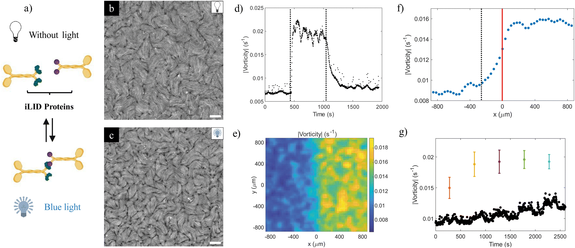

Fig. 1 Characterization of the light response of the photosensitive active nematic. (a) Photosensitive kinesins were developed by fusing iLID proteins (iLID in green and micro protein in purple) with kinesins. Under blue light, the iLID protein changes its conformation and binds to the microprotein, resulting in kinesin dimerization. Without light, the iLID protein returns to its inactivated state, breaking the dimer. (b) and (c) Fluorescence microscopy images of the resultant photosensitive active nematic without light (b) and with blue light (c). See also Movie S1a (ESI†). The scale bar is 100 μm. This experiment is performed with the highest ATP concentration, see Section 3.1. The light power density in the ON state is ca. 17 mW cm⁻². (d) Vorticity evolution (in absolute value) of the photosensitive material in Movie S1b (ESI†), showing light activation (t = 450 s) and deactivation (t = 1050 s). (e) and (f) Transition between a half-illuminated half-non-illuminated field of view for the data in Movie S1c (ESI†). The vorticity of the photosensitive active nematic at each position is time-averaged for 1 hour (e), and then it is averaged along the y position to obtain the activity profile in the frontier between the illuminated and non-illuminated areas (red line) (f). The end of the smooth transition between both regions is indicated with the black dashed line, which corresponds to the position where the vorticity attains the average value in the non-illuminated region plus its standard deviation. (g) Changes in the average vorticity of the material when undergoing cycles where a square region of increasing size is illuminated for 250 s, alternated with 250 s of relaxation in the dark. Black dots represent the mean vorticity in the non-illuminated area, while coloured dots represent the mean vorticity in the illuminated area, which is a square of size 200 μm (orange), 300 μm (yellow), 450 μm (purple), 600 μm (green), and 750 μm (purple). Mean values correspond to an average over space and time for a single experiment. Error bars are the standard deviation of the mean.

The first set of reported results refers to the characterization of the response of the photosensitive active nematic (AN) under illumination in its conventional turbulent regime.²⁹ Fluorescence microscopy images of an unconstrained (i.e. non-laterally confined) sample without and under blue light excitation are respectively shown in panels (b) and (c) in Fig. 1. It is noticed that, in our setup, excitation and fluorescence imaging are performed simultaneously. As a result, the illuminated pattern is always restricted to the field of view. Direct observation permits concluding that the speed of the AN (see Fig. S1 and S2, ESI†) and the density of defects both increase following illumination, in accordance with previous results.²⁸ This is easily rationalized since the former has been conjectured to follow in the turbulent regime an α^1/2 scaling,³² with α denoting the activity parameter. On the other hand, the density of defects is an inverse measure of the active length scale, generally accepted to scale as l_a ∝ α^−1/2.

From a quantitative point of view, flows in the AN turbulent regime are often gauged in terms of a mean vorticity, ω = ∂v_x/∂y − ∂v_y/∂x.³² In our experience, this is a more stable assessment of the local activity than speed, which is more prone to large amplitude temporal fluctuations. In Fig. S2 (ESI†), we show the average steady-state speed and vorticity values as a function of the applied power density. While both change similarly, we observe that the relative dispersion in the speed measurements is roughly twice that in vorticity measurements. The temporal change of the spatially averaged vorticity before and after an interval of illumination, as shown in panel (d), permits the characteristic time scales of excitation/de-excitation to be extracted. Both scales are in the range of minutes, although, as it is also apparent from the plot, forward and backward steps are substantially asymmetric. Indeed, while the excitation time is around 30–45 seconds, de-excitation is much slower, with the system losing around 80% of its speed in the first two minutes, and reaching the baseline (no light) state within an additional three minutes. It is also important to remark at this point that neither under the conditions of the experiment shown in Fig. 1, nor under other investigated conditions referred to later, the system complies with what would correspond to an ideal on/off switch (i.e. moving vs. rest state). This issue is inherent to the used kinesin proteins, as they have a tendency to form homodimers, which are able to power the active material in the absence of light, albeit in a less efficient way that the light induced heterodimers. This is evidenced in Fig. 1b and in the corresponding Movie S1 (ESI†), where turbulent flows and moving topological defects are present under dark conditions. Experimental results (not shown) obtained from testing each kinesin individually support this hypothesis. Recently, Zarei et al.²⁸ reported a true on/off behavior with a formulation based on a different kinesin.

Spatial scales can be similarly assessed, as shown in the remaining panels of Fig. 1. In panel (e), we plot the time averaged vorticity field for a prolonged illumination of half the system. More interesting is the corresponding panel (f), where the vorticity distribution is resolved spatially in terms of the distance to the boundary between illumination and non-illuminated regions. The transition between the illuminated and dark AN regions is not sharp. In this specific context, we define a penetration depth, λ, as the distance from the sharp boundary that separates the illuminated and non-illuminated regions (we refer to this as x = 0) into the dark region until the AN vorticity attains its non-illuminated value. We can estimate λ as the average AN speed, v, times the de-excitation time, t_OFF. In this example (highest ATP concentration), v = 2.3 ± 0.3 μm s⁻¹ and t_OFF ≃ 2 min, which results in λ = (2.8 ± 0.4) × 10² μm, consistent with the value of 250–300 μm obtained from the data in panel (f). In Fig. S3 (ESI†), we show the consistency of this estimation for experiments performed for different ATP concentrations, which yield different average speeds of the illuminated region. The penetration of activated flows in this design is unavoidable due to the material exchange between the illuminated and non-illuminated regions, which explains the smooth transition between the two regimes. Finally, panel (g) includes time plots of spatial averages of vorticity inside and outside the illuminated area, after illuminating square areas of increasing size. We observe that illuminated motifs with sizes smaller than 300 μm fail to achieve the maximum average vorticity, congruently with the penetration length identified earlier.

Recent studies by Zhang et al.³³ using a photosensitive actin/myosin active nematic system showed that, in their system, defects proliferating in the high activity region were confined by the boundaries of illumination patterns, which allowed defining activity tracks to guide defect self-propulsion. In their study, these authors reported a three-fold speed increase in the excited active flows when compared with the dark state, which is comparable to what we observe here (see Fig. S1, ESI†). A similar virtual confinement of defects was reported by Thijssen et al.¹² when they studied the same AN material that we study here while flowing over aqueous layers of different depths. Our experiments, however, do not show a similar contrast in the defect density in the high and low activity regions. To assess this, we have computed the topological charge density³⁴ for one experiment performed at the highest ATP concentration when half the field of view is illuminated (Fig. 2a and b) and have found that both its positive and negative values concentrate at the interface between the illuminated and non-illuminated regions in the steady state. Our measurements show that, in this experiment, the average topological charge densities are 3 ± 0.1 × 10⁻⁵ μm⁻² in the illuminated region and 2.5 ± 0.2 × 10⁻⁵ μm⁻² in the non-illuminated regions, while it reaches values close to 3.5 μm⁻² in the boundary region (defined as ±150 μm around x = 0, consistent with the magnitude of λ defined above). We have also explored the possibility to guide defects along activity tracks, but we have found that defects normally cross the activity boundary. Finally, we have tested whether the boundary between regions of different activities was able to polarize defects, as has been predicted in the literature.³⁵ For this purpose, we have measured the orientation of +1/2 defects in the dark, illuminated, and boundary regions in a half illuminated region. As shown in Fig. 2c–f, the defect orientation is roughly isotropic far from the interface, but is significantly polarized in the interfacial region, with defects predominantly oriented from the illuminated region towards the non-illuminated region. This result is consistent with the impossibility to confine defects with high activity tracks, as the former would be attracted, rather than repelled, by the boundary.

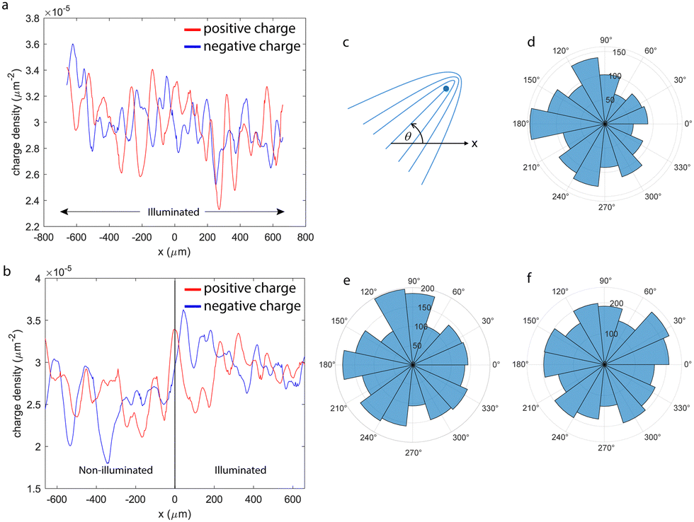Fig. 2 Distribution of charge density and defect polarization. (a) Profile of the average positive and negative topological charge density along the horizontal direction in a fully illuminated region. (b) Charge density profiles when the right half of the field of view is illuminated. Data correspond to averages over time and along the vertical spatial direction (parallel to the dark/bright interface when partially illuminated). (c)–(f) Radial histograms for the orientation of +1/2 defects, as defined in panel (c). Radial units are the number of defects. Data correspond to the transition (d), dark (e), and illuminated (f) regions.

The effect of a spatially distributed activity is better exemplified in Fig. 3. The illumination pattern is sketched above each panel, with white, gray, and black regions corresponding, respectively, to the illumination power to achieve 100%, 50%, and 0% of the photoenhancement (Fig. S2, ESI†). Spatial and temporal averages of the vorticity field are indicated for each of the elements in each pattern, as well as the global average value. We observe a trend where the contrast between the average vorticity inside bright and dark regions lowers as patterns become finer and, surprisingly, the average vorticity is also brought down. Even the central cell in the 3 × 3 pattern panel, whose average illumination coincides with that of the reference (top-left) panel, depicts, in comparison, a smaller value of vorticity. This observation is consistent with the idea that the full development of the AN activity is affected by lateral confinement,¹⁰ which decreases the average AN speed and vorticity. Our observations here indicate that a similar effect is obtained when confinement is the result of activity patterning. This is in contrast with the recent observation by Bate et al. with an active gel that features a truly on/off behavior,²⁰ where a checkerboard distribution of activity enhances the mixing of a dispersed passive dye. These observations suggest that, in our case, the mismatch between the different length and time scales in regions with different, but finite, activity plays a significant role in hindering the intrinsic evolution of the more active layer.

Fig. 3 Effect of a pattern of distributed activity. Different light patterns are applied always with the same average activity input. To compare the results between experiments, the vorticity is normalized using the averaged vorticity in the absence of light. The gray color represents illumination with the power density that produces half of the velocity growth (see Fig. S2, ESI†). Experiments are performed in the same region of each AN film. Each panel includes the vorticity map and the normalized values of vorticity, averaged over time and space and for 7 different films. Vorticity values are expressed in s⁻¹. See also Movie S2 (ESI†). Field of view, 1.7 × 1.7 mm².

3.2. Light control of confined flows

We report next the effects of distributed illumination on steered flows, i.e., situations where the normally isotropic active turbulent flows have been forced to move in a specified direction through external interventions. First, we consider a situation of geometrically confined AN. We choose to work with annular geometries as shown in Fig. 4 to avoid end effects.¹¹ It has been reported that narrow channels force symmetry breaking of the turbulent currents, with active flows developing a randomly chosen handedness, either clockwise (CW) or counter clockwise (CCW), while large channels maintain the isotropic, disordered flows. As the threshold width leading to symmetry breaking should be related to the active length scale of the AN, and the latter varies with the activity input, we have considered the possibility to reversibly alternate between the transport and the turbulent regimes by means of patterned illumination. In the current experiments, flow handedness is randomly chosen upon in situ polymerization of a ring-shaped channels. To easily visualize the flow handedness, we have resorted to constructing kymographs by stacking the fluorescence intensity profile along the center of the ring for different times, as shown in Fig. 4a. The presence of slopes on the kymograph patterns will indicate the handedness and magnitude of the active flow. In Fig. 4b, we show one example with a ring channel that has a spontaneous CW circulation. Global illumination of the system leads to a clear acceleration of the flow velocity, which reverts back to the original value once light is switched off and the system relaxes, always maintaining the same handedness. In Fig. 4d, we show a ring whose flow is turbulent (no net transport detected in the kymograph). We illuminate half of the ring, and we observe that the activated half develops the CW flow, but so does the non-illuminated half. The azimuthal component of the average velocity is roughly the same in both regions, consistent with mass conservation (Fig. S4a, ESI†). However, the average speed is about 50% higher in the illuminated region (Fig. S4b, ESI†). This additional activity is in the form of turbulent transversal flow (Fig. S4c, ESI†) and does not contribute to the net transport. When light is switched off, the system remains in a state of a slow CW flow. We found, thus, that once the symmetry is broken, the handedness is maintained even at low activities.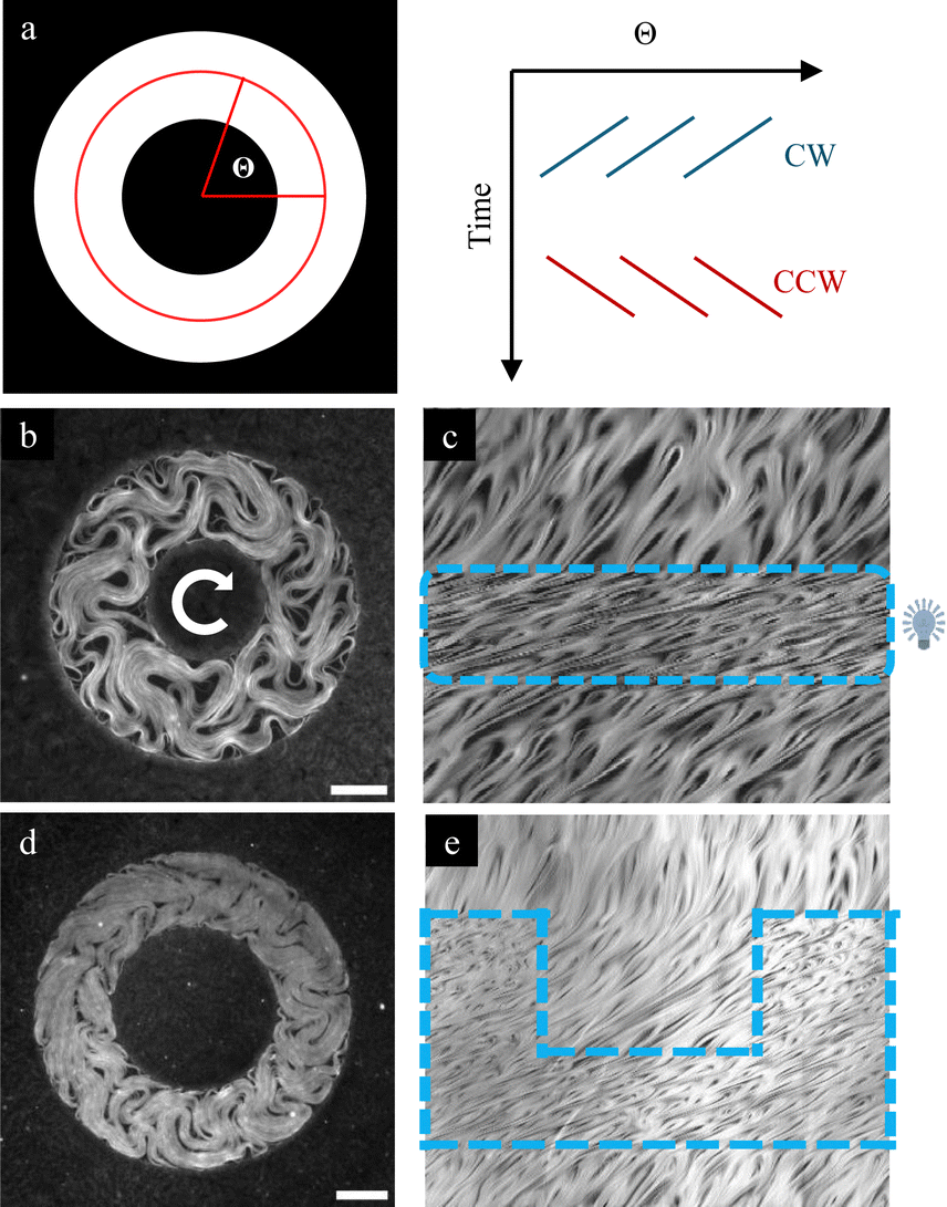

Fig. 4 The photosensitive active nematic confined in annular channels. (a) Schematic representation of a kymograph. The central section (red circumference) of the annular channel (averaged on a ring of radial width = 10 μm) is plotted over time. In the kymograph, traces appear directed to the left if the transport is clockwise (CW, blue) or to the right if it is counter clockwise (CCW, red). (b) and (d) Fluorescence images of the photosensitive material confined in annular channels of width: 170 μm (b) and 140 μm (d). (c) and (e) Kymographs of the corresponding experiments. In b, the full channel is illuminated, while in (d), only half is illuminated. See also Movies S3 and S4 (ESI†). The white arrow in the centre indicates the handedness of the motion, and the blue windows represent the spatiotemporal illumination pattern of the material. Light activation leads to the acceleration of transport, shown as more horizontal kymograph traces. The scale bar is 100 μm.

3.3. Light-induced flow alignment

Finally, we consider the effect of an activity boost on a regime of aligned, rather than turbulent, flows (Fig. 5). To this end, we interfaced the AN with an aligned passive liquid crystal layer in the high viscous anisotropy Smectic-A phase.¹⁷ This preparation results in the formation of an easy flow direction that leads to the reorganization of the AN, since the flow in the perpendicular direction is severely hindered. In Fig. 5a, we show an aligned AN layer with the full field of view illuminated, thus in the most excited state. In this regime, the flow organizes in aligned antiparallel channels where moving defects are preferentially located, separated by stripes where the fluorescence active filaments are concentrated. The width of these stripes was reported to change with α^−1/2, where α is the activity coefficient.¹⁷ Based on these earlier observations, we proceed to explore the contrast between the illuminated and non-illuminated regions by only exciting the top half of the field of view, so that the boundary between both regions is perpendicular to the flow alignment direction and to the stripes (Fig. 5b). In a different experiment, we only excite the right half of the field of view, so that the boundary is now parallel to the alignment direction (Fig. 5c). The speed is always faster in the illuminated region by a factor of 2, approximately. However, no significant difference is detected in the stripe widths in either case. In a previous study, we found that the average speed in the aligned regime scales with α.¹⁷ Therefore, one would expect the stripe width, which scales with α^−1/2, to change by around 30%. This may not be readily observable in our experiment. The fact that the field of view is surrounded by a much larger aligned and non-illuminated region likely hampers the reorganization of the aligned stripes upon illumination of the field of view.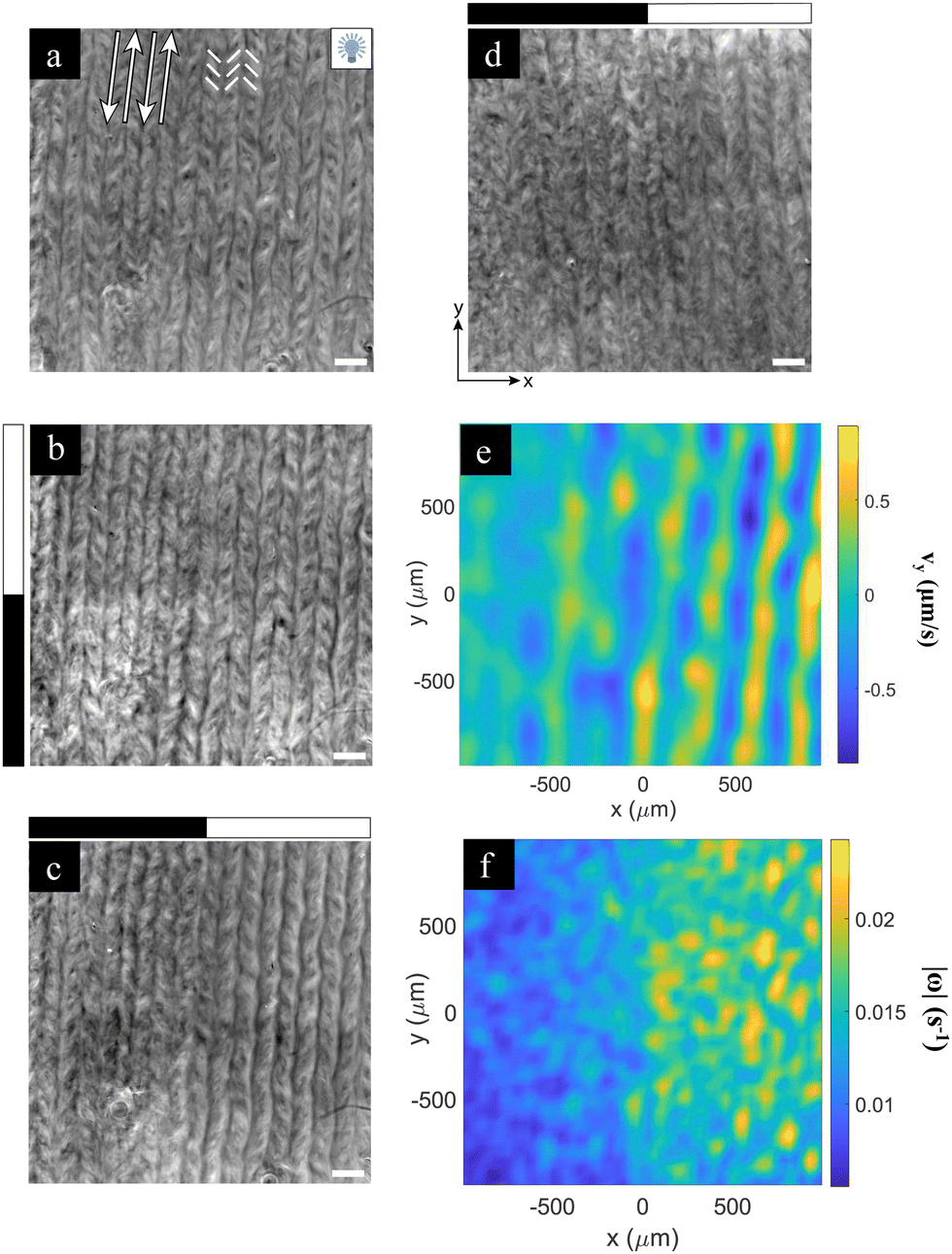

Fig. 5 Photoactivation of aligned flows. (a) The fluorescence image of the aligned material under light activation. White arrows indicate the direction of antiparallel flow lanes that separate fluorescent stripes. The underlying smectic-A planes (easy flow direction) is parallel to these arrows. White segments indicate the approximate orientation of the nematic director field, which attains a chevron-like pattern. (b) and (c) Fluorescence images of the aligned material when a half-dark half-bright pattern is applied perpendicular (b) or parallel (c) to the alignment direction. (d) The fluorescence image with the half-dark half-bright patterns parallel to the alignment direction of a system prepared at one tenth the normal ATP concentration. The scale bar is 200 μm. In panels (b)–(d), the black/white rectangular bands on the left or on the top of the image indicates which half of the system is illuminated (white). (e) and (f) The y-component of the velocity (e) and the vorticity (f) are analysed using PIV for experiments (d). See also Movie S5 (ESI†).

On the other hand, flow alignment due to interfacial anisotropy only takes place at high enough activity levels. In Fig. 5d, we have performed an experiment at 10% the normal activity, which is slightly below the level to achieve the proper flow alignment. When we illuminate the right half of the field of view, the activity boost triggers the flow alignment in that region. This can be assessed in the velocity (Fig. 5e) and vorticity (Fig. 5f) maps, where we observe that flows in the illuminated region are more ordered. In the experiment in Fig. 5d, we found 〈|V_x|〉 = 0.21 ± 0.04 μm s⁻¹ and 〈|V_y|〉 = 0.33 ± 0.05 μm s⁻¹ for the illuminated region, showing that the flow along the vertical direction is favored. For the non-illuminated region, we found 〈|V_x|〉 = 0.14 ± 0.03 μm s⁻¹ and 〈|V_y|〉 = 0.14 ± 0.03 μm s⁻¹, indicating that the system is still in its isotropic turbulent state (see Fig. S5, ESI†). This proves that we have been able to reversibly control an alignment transition in the AN layer by tuning the systems’ activity through the photosensitive motors. In the future, it will be interesting to analyze the nature of this transition, and compare it with recent studies using a direct control of viscous anisotropy that suggested that such an alignment transition is intrinsically first order.³⁶

4. Conclusions

In this work, we have studied the conventional active nematic system prepared from the assembly of microtubules and kinesins when forced under patterns of distributed activity. This is achieved by working with a motor protein preparation that can be reversibly excited with blue light. If a uniform activity boost is provided to the system, we observed an increase in the flow speed and a reduction of the intrinsic length scale, consistent with earlier studies. We have also found that interfaces between high and low activity regions induce a net polarization to +1/2 defects, which orient preferentially towards the low activity region. The lack of a truly on–off behavior, since active flows appear in the absence of illumination, likely prevents the effective confinement of defects in the more active regions and does not trigger the collective flow organization observed in confinement scenarios. Interestingly, we observe a reduced enhancement of the active flows when the illumination is spatially distributed, rather that uniformly applied. This indicates that lateral confinement effects, which lead to a decrease in the intrinsic length scale and in the flow speed, can be the result of activity patterning, not requiring physical confinement by rigid boundaries as previously demonstrated. We have also been able to leverage the provided activity boost to force a reversible transition between the isotropic turbulent and a regime of aligned flows, by preparing the active layer with low basal activity and in contact with an oil interface with high viscous anisotropy. The use of a photosensitive active nematic has a high potential for complex flow control and patterning in microfluidic applications, as we have shown using ring-shaped channels. However, to unleash the full potential of these capabilities, more responsive variants of the photosensitive microtubule system should be investigated, providing a truly arrested dynamics in the absence of external excitation.

In a broader context, by establishing a parallelism between activity and excitability, we might seek a connection between our current results and those reported in the past in relation to a photosensitive variant of the Belousov–Zhabotinskii reaction operated in its excitable regime.³⁷ Conclusions are certainly at odds when comparing both scenarios. In the latter case, a pattern of spatially distributed excitability favors pattern formation and even anticipates the corresponding instability of the rest state below threshold. Here, the reverse occurs as active flows are, on average, significantly slowed down when similarly actuated with illumination patterns. This points to profound differences between these two non-equilibrium systems. Excitability emerges in reaction-diffusion driven systems as locally elicited wave patterns. Conversely, active soft condensed matter systems respond in the form of self-organized textures and flows whose coherence can be jeopardized by spatially distributing the activity.

Author contributions

F. S. and J. I.-M. conceived the research. I. V. performed the experiments and analyzed the data. F. S. prepared the first draft. F. S. and J. I.-M. wrote the paper with input from all authors.

Data availability

All raw data and analysis codes are available from the corresponding author upon reasonable request.

Conflicts of interest

There are no conflicts to declare.

Acknowledgements

The authors are indebted to the Brandeis University MRSEC Biosynthesis facility for providing the tubulin and to T. D. Ross (Caltech/MIT) for providing the plasmid to express the photosensitive kinesins. We thank A. Espargueró, M. Pons, and R. Sabaté (Universitat de Barcelona) for their assistance in the expression of motor proteins. The authors thank A. Fernández-Nieves (University of Barcelona) for sharing the defect detection code. I. V.-C. acknowledges funding from Generalitat de Catalunya though a FI-2020 PhD Fellowship. I. V.-C., J. I.-M., and F. S. acknowledge funding from MICIU/AEI/10.13039/501100011033 (Grant PID2022-137713NB-C21). I. V.-C. and J. I.-M. acknowledge funding from MICIU/AEI/10.13039/501100011033 (Grant No. PDC2022-133625-I00). Brandeis University MRSEC Biosynthesis facility is supported by NSF MRSEC 2011846.

Notes and references

1. S. Ramaswamy, Annu. Rev. Condens. Matter Phys., 2010, 1, 323–343.
2. M. C. Marchetti, J. F. Joanny, S. Ramaswamy, T. B. Liverpool, J. Prost, M. Rao and R. Aditi Simha, Rev. Mod. Phys., 2013, 85, 1143–1189.
3. G. Gompper, et al. , J. Phys.: Condens. Matter, 2020, 32, 193001.
4. F. Sagués, Colloidal Active Matter, Taylor and Francis Group, Boca Raton, FL, 2023.
5. M. M. Norton, P. Grover, M. F. Hagan and S. Fraden, Phys. Rev. Lett., 2020, 125, 178005.
6. T. Sanchez, D. T. N. Chen, S. J. Decamp, M. Heymann and Z. Dogic, Nature, 2012, 491, 431–434.
7. J. Prost, F. Jülicher and J. F. Joanny, Nat. Phys., 2015, 11, 111–117.
8. K. T. Wu, J. B. Hishamunda, D. T. N. Chen, S. J. DeCamp, Y. W. Chang, A. Fernández-Nieves, S. Fraden and Z. Dogic, Science, 2017, 355, eaal1979.
9. A. Opathalage, M. M. Norton, M. P. N. Juniper, B. Langeslay, S. A. Aghvami, S. Fraden and Z. Dogic, Proc. Natl. Acad. Sci. U. S. A., 2019, 116, 4788–4797.
10. J. Hardoüin, R. Hughes, A. Doostmohammadi, J. Laurent, T. Lopez-Leon, J. M. Yeomans, J. Ignés-Mullol and F. Sagués, Commun. Phys., 2019, 2, 1–9.
11. J. Hardoüin, J. Laurent, T. Lopez-Leon, J. Ignés-Mullol and F. Sagués, Soft Matter, 2020, 16, 9230.
12. K. Thijssen, D. A. Khaladj, S. A. Aghvami, M. A. Gharbi, S. Fraden, J. M. Yeomans, L. S. Hirst and T. N. Shendruk, Proc. Natl. Acad. Sci. U. S. A., 2021, 118, 1–10.
13. J. Hardoüin, C. Doré, J. Laurent, T. Lopez-Leon, J. Ignés-Mullol and F. Sagués, Nat. Commun., 2022, 13, 6675.
14. F. Keber, E. Loiseau, T. Sanchez, S. DeCamp, L. Giomi, M. Bowick, M. C. Marchetti, Z. Dogic and A. Bausch, Science, 2015, 345, 1135–1139.
15. P. W. Ellis, D. J. G. Pearce, Y.-W. Chang, G. Goldsztein, L. Giomi and A. Fernandez-Nieves, Nat. Phys., 2018, 14, 85–90.
16. P. Guillamat, Ž. Kos, J. Hardoüin, J. Ignés-Mullol, M. Ravnik and F. Sagués, Sci. Adv., 2018, 4, eaao1470.
17. P. Guillamat, J. Ignés-Mullol and F. Sagués, Proc. Natl. Acad. Sci. U. S. A., 2016, 113, 5498–5502.
18. P. Guillamat, J. Ignés-Mullol and F. Sagués, Nat. Commun., 2017, 8, 564.
19. G. Sarfati, A. Maitra, R. Voituriez, J. C. Galas and A. Estevez-Torres, Soft Matter, 2022, 18, 3793–3800.
20. T. E. Bate, M. E. Varney, E. H. Taylor, J. H. Dickie, C. C. Chueh, M. M. Norton and K. T. Wu, Nat. Commun., 2022, 13, 6573.
21. M. Nakamura, L. Chen, S. C. Howes, T. D. Schindler, E. Nogales and Z. Bryant, Nat. Nanotechonol., 2014, 9, 693–697.
22. M. D. Yamada, Y. Nakajima, H. Maeda and S. Maruta, J. Biochem., 2007, 142, 691–698.
23. G. Guntas, R. A. Hallett, S. P. Zimmerman, T. Williams, H. Yumerefendi, J. E. Bear and B. Kuhlman, Proc. Natl. Acad. Sci. U. S. A., 2015, 112, 112–117.
24. T. D. Ross, H. J. Lee, Z. Qu, R. A. Banks, R. Phillips and M. Thomson, Nature, 2019, 572, 224–229.
25. Z. Qu, D. Schildknecht, S. Shadkhoo, E. Amaya, J. Jiang, H. J. Lee, D. Larios, F. Yang, R. Phillips and M. Thomson, Commun. Phys., 2021, 4, 198.
26. L. M. Lemma, M. Varghese, T. D. Ross, M. Thomson, A. Baskaran and Z. Dogic, PNAS Nexus, 2023, 2, 1–10.
27. B. Najma, M. Varghese, L. Tsidilkovski, L. Lemma, A. Baskaran and G. Duclos, Nat. Commun., 2022, 13, 6465.
28. Z. Zarei, J. Berezney, A. Hensley, L. Lemma, N. Senbil, Z. Dogic and S. Fraden, Soft Matter, 2023, 19, 6691–6699.
29. A. Doostmohammadi, J. Ignés-Mullol, J. M. Yeomans and F. Sagués, Nat. Commun., 2018, 9, 3246.
30. I. Velez-Ceron, P. Guillamat, F. Sagues and J. Ignes-Mullol, Proc. Natl. Acad. Sci. U. S. A., 2024, 121, e2312494121.
31. P. W. Ellis, J. Nambisan and A. Fernandez-Nieves, Mol. Phys., 2020, 118, 1–9.
32. L. Giomi, Phys. Rev. X, 2015, 5, 031003.
33. R. Zhang, S. A. Redford, P. V. Ruijgrok, N. Kumar, A. Mozaffari, S. Zemsky, A. R. Dinner, V. Vitelli, Z. Bryant, M. L. Gardel and J. J. de Pablo, Nat. Mater., 2021, 20, 875–882.
34. M. L. Blow, S. P. Thampi and J. M. Yeomans, Phys. Rev. Lett., 2014, 113, 248303.
35. S. Shankar and M. C. Marchetti, Phys. Rev. X, 2019, 9, 041047.
36. O. Bantysh, B. Martínez-Prat, J. Nambisan, A. Fernández-Nieves, F. Sagués and J. Ignés-Mullol, Phys. Rev. Lett., 2024, 132, 228302.
37. S. Alonso, I. Sendiña-Nadal, V. Pérez-Muñuzuri, J. M. Sancho and F. Sagués, Phys. Rev. Lett., 2001, 87, 078302.

---

Footnote

† Electronic supplementary information (ESI) available. See DOI: https://doi.org/10.1039/d4sm00651h

---