 Open Access Article
Random field reconstruction of three-phase polymer structures with anisotropy from 2D-small-angle scattering data†
Stephen
Kronenberger
 a,
Nitant
Gupta
 a,
Benjamin
Gould
b,
Colin
Peterson
b and
Arthi
Jayaraman
 *acd
*acd
aDepartment of Chemical and Biomolecular Engineering, University of Delaware, Colburn Lab, 150 Academy Street, Newark, DE 19716, USA. E-mail: arthij@udel.edu
bThe Chemours Company, 201 Discovery Blvd, Newark, DE 19713, USA
cDepartment of Materials Science and Engineering, University of Delaware, Pierre S. Du Pont Hall, 127 The Green, Newark, DE 19716, USA
dData Science Institute, University of Delaware, Newark, DE 19716, USA
First published on 14th October 2024
Abstract
In this paper we present a computational method to analyze 2-dimensional (2D) small-angle scattering data obtained from phase-separated soft materials and output three-dimensional (3D) real-space structures of the three types of domains/phases. Specifically, we use 2D small-angle X-ray scattering (SAXS) data obtained from hydrated NafionTM membranes and develop a workflow using random fields to build the 3D real-space structure comprised of amorphous hydrophilic domains, amorphous polymer domains, and crystalline polymer domains. We demonstrate the method works well by showing that the reconstructed 3D NafionTM structures have a computed scattering profile that matches the input experimental scattering profile. Though not demonstrated in this work, such reconstructions can be used for further analysis of domain shapes and sizes, as well as prediction of transport properties through the structure. Our method in this work extends capabilities beyond the previously published random field small angle scattering reconstruction method introduced by Berk [Phys. Rev. Lett. 1987, 58 (25), 2718–2721] that had been used to reconstruct structures from 1D small angle scattering data of two-phase systems. The method in this work can be used to generate isotropic, two-phase reconstructions, but can also handle 2D SAXS profiles from three-phase systems that have structural anisotropy resulting from material processing effects.
Introduction
Small-angle scattering (SAS) measurements are widely used to investigate the structure of polymeric/oligomeric soft materials. In a SAS experiment, a beam of X-rays (SAXS) or neutrons (SANS) is passed through the sample, and a detector measures the intensity of the scattered beam at different azimuthal angles (θ), and the magnitudes of scattered wavevectors (q). This results in a 2-dimensional (2D) scattering pattern, with the intensity of scattered neutrons or X-rays being measured as a function of q and azimuthal angle θ, or equivalently as a function qx and qy, which are the scattered wavevector magnitudes measured along the instrument axis frames. When there is no global structural anisotropy within the material, the 2D scattering pattern is symmetric about its center, and the data is typically azimuthally averaged over θ to a 1-dimensional (1D) scattering profile, I(q). When there is structural anisotropy within the material, then the 2D scattering profile is not radially symmetric and azimuthal averaging can lead to loss of the information regarding the structural anisotropy.SAXS and SANS measurements benefit from requiring less sample preparation than direct-imaging techniques such as scanning and transmission electron microscopy (SEM/TEM) or atomic force microscopy (AFM) where sample preparation can alter the structure of the material of interest. Moreover, while such direct-imaging techniques provide a real-space view of a section of the material structure, SAS provides structural information across multiple length scales ranging from 1–100 nanometers, typically covering a larger portion of the material. SAS achieves this by recording structural information in the reciprocal (or Fourier) space, which is effective in compressing information to the most relevant structural correlations. However, the interpretation of such reciprocal-space measurements, especially while considering the complete 2D scattering profiles, is not always straightforward and requires additional processing.
For azimuthally averaged 1D scattering profiles, I(q) vs. q, of polymeric and soft materials, transformations in the form of Guinier, Porod, or Kratky plots can be constructed. These transformations reveal the slope or asymptotic behavior of the scattering profiles to extract information such as the radius of gyration of particles or polymeric chains and mass or surface fractal dimensions.1,2 If the forms (or particle shapes) within the material structure are well understood, relevant analytical models can be fit to the scattering data to provide estimates of the average particle dimensions. Fitting to such analytical models for particle forms that are relevant in polymeric and soft materials (including spheres,3 cylinders,4 flexible cylinders,5 lamellae,6 rectangular prisms,7 and others) is often facilitated by user-friendly software such as SASView (https://www.sasview.org/).
On the other hand, to interpret scattering profiles obtained from structures that do not have relevant analytical models, computational methods such as Computational Reverse-Engineering Analysis for Scattering Experiments (CREASE) enable optimization of structural features (e.g., distributions of domain shapes, sizes, orientation, etc.) whose computed scattering profile matches with the experimental scattering profile.8–12 CREASE also outputs the three-dimensional (3D) structures corresponding to those structural features; 3D structures are valuable for visualization purposes as well as for use in other computational techniques to predict macroscale properties.
Some other methods of SAS analysis focus on perturbing a 3D structure to drive its computed scattering profile towards an experimental scattering profile. Broadly, these techniques involve iteratively computing the scattering profile (or analogously the two-point correlation function) of a structure and then accordingly modifying the 3D structure through optimization to obtain a better match between the computed and experimental scattering profiles. Some prominent examples of these methods include Yeong and Torquato's method based on “stochastic optimization,” Franke and Svergun's DAMMIF method and Seibert et al.'s MCRpy method.13–15
Apart from methods that rely on optimization-based approaches to reconstruct 3D structures from scattering profiles, a more direct approach is to transform the measured scattering profile into the corresponding 3D structure. This is possible by utilizing random fields (RFs) and has been demonstrated earlier for 1D SAS profiles. RFs are spatially varying, statistically random fields, whose values may follow a distribution. One common class of random fields are Gaussian random fields (GRFs), where the field values follow a Gaussian distribution. This work only concerns GRFs, so we use the terms “random field” or “RF” interchangeably with GRF. Additionally, the field values have a well-defined spatial correlation (or covariance) relationship. Typically, while using RFs to reconstruct material structure from scattering data, the continuously varying RF values are first thresholded at a specified cutoff value called the “level cut” (which we shall denote as α). The regions of the field that are greater than α represent phase 1, while the regions less than α represent phase 2. Consequentially, the volume fraction of the two phases is controlled by the level cut value α. Because of their flexibility, random fields have been used in a wide range of spatial modeling applications, including geological estimation, astronomy, and brain mapping.16–21
In soft materials, RFs were first proposed to model structures by Cahn,22 and the method was later formalized for a method of analyzing scattering data by Berk.23,24 Since then, RFs have been used to model microemulsions of water, oil, and surfactant from scattering data23,25 and are consistently being developed to model a wide range of materials including gels, aerogels, nanoparticles, and porous materials.26–29 Such developments include constructing structures as a combination of multiple random fields to allow greater diversity in the patterns of structures that can be generated.29 Additionally, random field structures have been generated by thresholding a field twice (with two “level cuts”) to enable three phase structures with the third additional phase acting as a boundary layer between the other two phases.23 Adjacently, “plurigaussian” random fields have been used to model 3-phase materials with different types of interfaces between the three phases.27
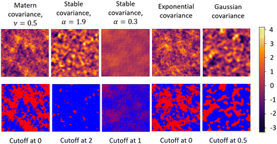
In Fig. 1, we show a variety of GRFs and their level-cut versions. As depicted, the visually perceived “pattern” of the GRF is specified by its covariance function C(r), which relates the relative position r of two points within the field to the covariance between the points’ values. The Fourier transform of C(r) gives the spectral density f(q) of the random field and is also used to specify the “pattern” of the GRF. Here, the spectral density, which describes the strength of the contribution of a given wavenumber q to the field value of the resulting GRF, is numerically analogous to the scattering intensity I(q) as measured in SAS experiments. It can be appreciated from the examples shown in Fig. 1, that the statistical properties of a level-cut GRF are completely specified by their level-cut value and the choice of the covariance function (or analogously by the spectral density).
In the application of RFs to reconstruct 3D structures from scattering profiles, one challenge that has not yet been addressed involves utilizing the full 2D scattering profile to model structures with anisotropy. 2D scattering profiles are particularly useful to interpret global anisotropy in material structures that can result from processing techniques. To the best of our knowledge, all RF reconstructions in the literature have assumed (or approximated) isotropic structural arrangement. Furthermore, RF-based approaches have so far not tackled the problem of reconstructing structures from a scattering profile that has multiple phases that can be separated across different length scales. Analyzing 2D scattering profiles and interpreting multiple phases separated across multiple length scales are highly relevant to a detailed interpretation of the structure of perfluorinated sulfonic acid (PFSA) ionomer membranes, such as NafionTM, which is one of the goals of this work.
PFSA ionomers are composed of a hydrophobic perfluorinated backbone, with side chains that are terminated with hydrophilic sulfonic acid groups. The PFSA chemistry results in the material being hygroscopic, while also undergoing a nano-phase separation between the hydrophobic polymer backbone and the hydrophilic domain composed of sulfonic acid groups and absorbed water. Additionally, the PFSA backbone can crystallize, resulting in a semi-crystalline matrix which, along with amorphous hydrophilic domains, are dispersed throughout the region composed of amorphous backbone chains. The semi-crystallinity gives the material desirable mechanical properties, while the interconnected hydrophilic domains allow for ion transport which makes PFSA ionomers an ideal material for ion transport membranes in various electrochemical applications.30 Despite a wide range of experimental and computational studies aimed at elucidating the molecular structure of PFSA ionomers, the structure of these membranes is still debated.31–35 Due to the difficulties with direct imaging of the structure of PFSA membranes, researchers have often turned to SAS to understand the membrane structure.36–39
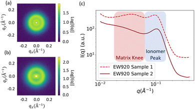
Generally, the SAS profile of PFSA membranes shows two major peaks. The peak at lower q, whose center typically falls outside the q range of interest and is therefore observed as a “knee” or “shoulder,” is called the matrix knee and is attributed to the spacing between crystalline domains. The peak at higher q is called the ionomer peak and is attributed to the structure of the hydrophilic domains. Fig. 2 shows examples of the 1D and 2D scattering profiles for PFSA membranes. 2D scattering profiles can display anisotropy from processing-induced structural anisotropy (Fig. 2b).
Typically, SAS measurements can have some degeneracy, and materials with different morphologies can, in theory, give rise to the same scattering profile. This ambiguity is readily apparent in previous SAS studies of PFSA ionomers, as several different types of structural models have been used to explain the scattering from PFSA ionomers. Among these models are the cluster-network model, the cylindrical model, and the locally flat network model.37,39,40 In the cluster-network model, it is assumed that at low hydration, water molecules cluster around the sulfonic acid groups; then, as the hydration increases, these clusters of water molecules grow and connect to form thin channels. In the cylindrical model, the hydrophilic domains’ structure is described as a series of locally parallel, cylindrical channels that grow as hydration increases. Finally, in the locally flat network model, the structure is described as a network of ribbon-like flat channels that become thicker as hydration increases. For brevity, we do not go into further detail about the broad range of work characterizing PFSA membranes and refer the reader to a detailed review by Kusoglu and Weber.30
In this work, we describe the development of our GRF-based 3D reconstruction of three-phase structures with or without anisotropy from 2D scattering profiles, while applying it to the experimental SAXS data of PFSA ionomers. Our focus in this paper is on the method for 3D real space structure reconstruction from scattering data. We first describe an extension of the random field reconstruction method to analyze anisotropic 2D scattering data, as well as, to account for the three phases—hydrophilic domains, amorphous polymer, crystalline polymer—by deconvoluting the contributions of the major peaks. We then demonstrate this method using experimental 2D SAXS data of hydrated NafionTM PFSA membranes provided by the Chemours Company. The motivation to use random fields, rather than cluster network or cylindrical morphologies, stemmed from our recent parallel efforts of computational exploration of the PFSA ionomers’ structure,41 where we conducted coarse-grained molecular dynamics simulations of self-assembly of PFSA ionomers for varying polymer designs (i.e., side chain length and spacing) and at increasing extents of hydration. Additionally, recent detailed experiments that directly imaged the hydrophilic domains within PFSA ionomer membranes showed connected networks with similar morphologies to random fields.42,43 The structures found in that study showed similarity to level-cut random fields across various quantitative structural measures (additional details provided in Section S1, ESI†), validating our choice to use random fields. We note that previous work by Aieta et al.44 has attempted to use a similar approach to reconstruct the structure of NafionTM membranes. However, their work was restricted to isotropic scattering profiles and only considered two phases, the hydrophilic domains and amorphous domains. As we demonstrate later, our developed method provides a 3D structural reconstruction with anisotropic information for all the three phases.
Method
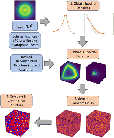
The workflow we have developed is described in Fig. 3. We describe each step of the workflow in detail in the following sub-sections. The details regarding the numerical implementation of each step are included in Section S2 (ESI†). Briefly, given an input 2D SAS scattering profile with two primary peaks and estimated values of the volume fractions for the three phases—hydrophilic domains, amorphous polymer and crystalline polymer—we first obtain a series of 1D scattering profiles that were averaged over equally spaced bins of azimuthal angles (θ) in the 2D scattering profile. We then deconvolute the two peaks (the matrix knee and the ionomer peak) from the 1D scattering profile at each angle θ. These deconvoluted peaks are then used to obtain their corresponding spectral densities, and subsequently two corresponding random fields. Finally, each of the random fields are level cut and combined into the final 3D structure. Due to the nature of this reconstruction, where we combine two separate random fields, it is important that the phases of interest can be considered independent of one another, as they will be independent in the final reconstruction.Obtaining spectral densities
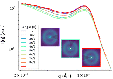
To obtain the spectral densities required to generate the random fields, we use the bin-averaged scattering profiles (Iθ(q)), one for each azimuthal direction (θ). In this work, we use angular slices (or intervals) of size Δθ centered at nθ angles evenly spaced from θ = [0,π], as illustrated in Fig. 4.We then fit each Iθ(q) to the functional form in eqn (1) which is the sum of two terms: Iθ,1(q) and Iθ,2(q). We adopted the first term Iθ,1(q) from the Debye–Beuche (DB) model to describe the matrix knee and the second term Iθ,2(q) from the Tuebner–Strey (TS) model to describe the ionomer peak.45,46 The fit parameters are ADB and ATS (scale parameters for the DB and TS terms, respectively), Ξ (correlation length of the DB term), and d and ξ (characteristic TS domain size and correlation length, respectively).
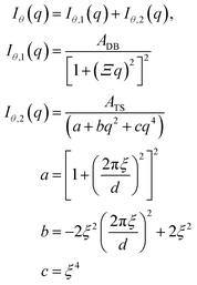 | (1) |
In the context of this deconvolution procedure, we emphasize again that the phases are considered to be independent of one another. As scattering occurs between all phases of the system, there will inherently be a cross-term in the actual scattering contribution of three phases that is not accounted for by a summation of two terms as we have used in eqn (1). However, if the length scales of the two different phases are sufficiently different, this cross-term becomes negligible, and eqn (1) will give a satisfactory fit to the experimental SAXS data.
When reconstructing level-cut RF structures from small-angle scattering data, the level-cut value (α) is determined using the cumulative distribution function for the Gaussian distribution with the volume fraction of one of the phases, say phase 1 (ϕ1), obtained from prior experimental knowledge about the system of interest (eqn (2)). When thresholding the RF, all field values above α become phase 1, while all field values below α become phase 2.
 | (2) |
First the Debye correlation function Γ(r) is computed from the input scattering profile I(q) (eqn (3).
 | (3) |
 | (4) |
| C11(r) = Γ(r)ϕ1(1 − ϕ1) | (5) |
 | (6) |
Finally, the spectral density f(q) of the random field can be computed from the Fourier transform of CRF(r) (eqn (7)).
 | (7) |
Processing spectral densities
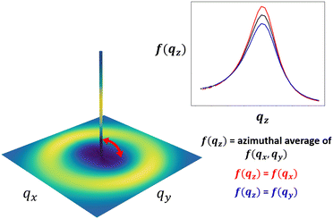
In an isotropic material structure, as the azimuthal angle θ is varied, every fθ,1(q) would be equivalent; the same would be true of each fθ,2(q). We could then directly proceed to generate the random fields used to reconstruct the material structure. However, in a material that exhibits structural anisotropy, the anisotropy is preserved in the discrete sets of fθ(q) across the azimuthal angles θ. We can interpolate these sets to get fθ(q) for any intermediate values of θ or q. This interpolation results in one 2D spectral density, f2D(qx, qy), for each peak. The 2D spectral densities can be used directly to create real-space reconstructions in two dimensions only. However, since we ultimately aim to generate 3D real-space structural reconstructions, which requires a 3D spectral density, we assume a spectral density in the third dimension f(qz) and interpolate between f(qz) and f2D(qx, qy) along the azimuthal angle to obtain our 3-dimensional spectral density, f3D(qx, qy, qz). This is illustrated schematically in Fig. 5, and additional details are provided in Section S2 (ESI†).In an experimentally obtained 2D scattering profile, the information about the structure or its anisotropy in the direction of the incident X-ray or neutron beam is not available. In such cases, complete information about the structural anisotropy can be obtained from additional scattering experiments along different axes of the material.48 However, for the case of NafionTM membranes, we can only perform scattering measurements where scattering beam is orthogonal to the surface of the membrane because the membranes are too thin to perform scattering experiments on the membrane's cross-section. For this reason, we assume that the spectral density in the third dimension is the overall azimuthal average of f2D(qx, qy). While this is likely not entirely accurate, this assumption could be further refined if additional information is known about the processing that gave rise to the anisotropy. For example, if the processing involves flow along the y-dimension, then it is reasonable to assume isotropy in the xz-plane, and setting f(qz) = f(qx) would be more reasonable. In the main body of this paper, we show the results assuming f(qz) is the azimuthal average of the f2D(qx, qy), and in Section S5 (ESI†), we include an example reconstruction with the assumption f(qz) = f(qx) for comparison.
Generating random fields
From the 3D spectral density, we generate random fields using eqn (8). | (8) |
 denotes the 3D fast Fourier transform and
  its inverse. W is an N × N × N array of noise sampled from the standard normal distribution. A is the 3D spectral density corresponding to the specific q values that are needed to generate a reconstruction of a given size and resolution. A is interpolated from the 3D spectral density obtained in Step 2 (Processing spectral densities). The array of q values used to interpolate A are determined by the frequencies corresponding to the discrete Fourier transform of the array. The size of the structural reconstruction (i.e., number of voxels making up one edge of the structural reconstruction, N) and resolution of the structural reconstruction (i.e., size of a voxel, a) are defined in this step, as they directly impact the q values used to construct A.
Because of the wide applicability of using random fields to model various phenomena, there have been many developments to simulating random fields in different ways.49 For completeness here, we include reference to the method that has been most frequently used previously to generate random field reconstructions from small-angle scattering data. In this method, RFs were generated by a summation of plane waves sampled from its defining spectral density f(q) (eqn (9)).23,25
 | (9) |
We use eqn (8) instead of eqn (9) for a few reasons. First, the RFs generated using eqn (8) are periodic, which is not the case of RFs generated using eqn (9). This better enables RFs generated using our method to be used for additional computational analysis, for example transport simulations or density-guided molecular dynamics simulations to obtain finer-resolution structures of chain conformations. Additionally, using eqn (9) has the drawback that one must sample from the spectral density. This is straightforward when sampling from a 1D spectral density but can become significantly more complex for the 3D spectral densities that we use to preserve the structural anisotropy. By contrast, eqn (8) only requires interpolation of the 3D spectral density, which is much more straightforward.
Eqn (8) is used to generate two random fields from the two 3D spectral densities that have been computed. These fields are in the form of 3D arrays, where each voxel (array entry) has a continuous value corresponding to the value of the field at that point.
Combining random fields to create final 3D structure
To combine the random fields into the final 3D structure reconstruction, we first threshold each random field by their corresponding level-cut values. We then superimpose the larger length-scale level-cut field (corresponding to the lower q range) onto the smaller length-scale level-cut field (from the higher q range). This superposition can be described using eqn (10): | (10) |
We choose this order of superposition rather than the opposite order to minimize the finite-size effects of the reconstruction. There will be fewer of the larger length-scale domains in the reconstruction, so changing their shape by superimposing the smaller length-scale field over the larger domains would result in more noise in the scattering from the poorer sampling of larger domains. In contrast, the smaller length-scale field is better sampled because there are more domains, so superimposing the larger length-scale field over them has a smaller effect on their contribution to the scattering. We illustrate this concept in Fig. S11 (ESI†).
Accounting for the superposition of the larger length-scale field over the smaller-length scale field, the volume fractions passed to the earlier steps of the method need to be updated so that the reconstruction volume fractions match the input volume fractions. Specifically, we need to overestimate the volume fraction passed to the smaller length-scale field (eqn (11)) to obtain the target volume fraction in the final reconstruction, since some of the domains will be covered by domains of the larger length-scale field.
 | (11) |
At the end of this process, we have one 3D array, with each voxel containing one of three discrete values, corresponding to the three phases in the material. As such, this is a relatively coarse representation of the material structure which gives the relative position of the different phases to one another. We note that the real space structural reconstruction does not contain molecular-scale information such as polymer chain conformation or locations of individual molecules. However, one could refill the molecular details in a manner similar to approaches used in the literature for regaining finer resolution in structures generated from field simulations.50
Application of method to NafionTM SAXS data
The procedure for collecting and preprocessing the experimental 2D SAXS data of NafionTM ionomer membranes used in this study is described in Section S3 (ESI†).Next we describe the various steps of the method described in Methods as they are applied to the input 2D SAXS data to generate the 3D reconstructed structure. We conclude this section with a validation of the method by comparing the input SAXS profiles to the computed scattering profiles calculated from the 3D reconstructed structure.
For reconstructing the 3D structure of NafionTM membranes, we wish to capture three phases: crystallite domains, amorphous domains, and hydrophilic domains (consisting of water, sulfonate ions, and aqueous cations).40,51 With regard to the crystallite domains, it is important to note that the information included in the SAXS matrix knee corresponds to the length scale of the crystallite domains rather than crystalline peaks that would indicate the atomic crystal structure within the crystallite domains. As such, in our reconstructions, we aim to resolve only the former. The peak deconvolution enables us to obtain two level-cut fields, one of each corresponding to the matrix knee and the ionomer peak. These level-cut fields individually provide information about the corresponding two-phase structures of the hydrophilic-amorphous domains (which we will call the ionomer peak field) and crystallite-amorphous domains (which we will call the matrix knee field), respectively.
We specify one volume fraction for each random field. For the ionomer peak field, we specify the fraction of hydrophilic domains (ϕhydrophilic), and for the matrix knee field, we specify the fraction of crystallite domains (ϕcryst). The remainder (1 − ϕhydrophilic − ϕcryst) corresponds to the volume fraction of the amorphous phase (ϕamorphous).
Applying our method above to the NafionTM SAXS data with these phase designations, we first take the bin-averaged intensity over nθ subsets of azimuthal angles of the 2D SAXS data. We find that choosing the value of nθ = 10 (angles) works well to balance the interpolation quality and computation time for this data. Additionally,  gives angular slices large enough to reduce the noise in Iθ(q) that is seen when using smaller angles. For other types of SAXS data, the above choices would likely need to be varied to obtain optimal results. Here one would first select Δθ by starting with small values and increasing Δθ until the noise in the angular scattering profiles is minimal, as indicated by a smooth scattering profile. The choice of Δθ is also dictated by the variability of the scattering data as a function of θ. For data with sharper peaks at different θ, this variability could be washed out if a large Δθ is used, and a smaller Δθ should be used. For data similar to ours, where the change in scattering as a function of θ is relatively minimal and smooth, larger Δθ can be used. Next nθ is selected as the smallest value for which we do not see any effects of further increasing nθ on the interpolated spectral density. When selecting Δθ and nθ, the angular slices do not need to perfectly cover the 2D scattering profile; the slices can overlap (as they do with our selected values).
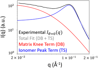
When deconvoluting each Iθ(q), its first peak corresponding to the matrix knee will be denoted with the subscript “matrix”, and the second peak corresponding to the ionomer peak and will be denoted with the subscript “ionomer”. Using our method of combining the random fields, the “matrix” peak corresponds to the difference in phase between the crystalline domains and the hydrophilic and amorphous domains of the membrane. The “ionomer” peak corresponds to the difference in phase between the hydrophilic domains and the amorphous polymer domains. We show the fit function compared with the experimental Iθ=0(q) in Fig. 6 to demonstrate the fit quality. The range of q values considered for the fitting is 0.02 to 0.2 Å−1.
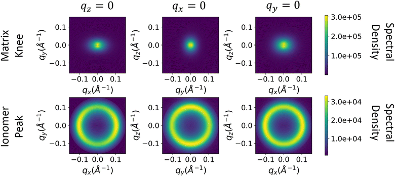
The spectral densities are then computed and interpolated as described in eqn (3)–(7) in Methods. We assume that the spectral density in the z-direction is equal to the azimuthal average of the 2D spectral density (Processing spectral densities sub-section of Methods). 2D slices along each axis of the resulting 3D spectral densities are shown in Fig. 7.
Finally, the random fields are generated and combined into the final voxelated structure. For each reconstructed structure, we compute the 1D and 2D scattering profiles using the fast Fourier transform.52,53 As the reconstruction includes three components, the X-ray scattering length densities (SLDs) and volume fractions of all three species will strongly impact the shape of the scattering profile. In this work, we utilize SLD values that were used in previous work performing computational reconstruction of NafionTM.51 These SLD values originate from previous SAXS experimental work,36 and have been used in several other studies that have modeled the structure of NafionTM membranes using computational methods.40,52 The fast Fourier transform scattering calculation and the specific values of SLDs used in this work are described in detail in Section S4 (ESI†).
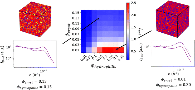
In Fig. 8, we show two 3D real-space structural reconstructions and their computed 1D and 2D scattering profiles. While the computation of the spectral densities preserves the general shape of the matrix knee and ionomer peak, different ratios of crystallite and hydrophilic volume fractions directly impact the relative intensities of these peaks in the computed scattering profile. The volume fractions need to be optimized to obtain the correct relative peak intensities.
This can be accomplished in a few different ways. First, if experimental determination of all volume fractions is straightforward, they can directly be used in the reconstruction. Assuming the chosen functional form for deconvolution and SLDs are valid, the reconstruction scattering will match that of the input scattering with the experimental volume fractions. If the volume fraction of one phase is obtainable, but not the others, information about the relative intensities of the scattering features can be used to obtain the volume fraction of the other phases such that the reconstruction scattering will match the input scattering. We demonstrate this case in the following paragraphs. In a final case where all volume fractions are difficult to accurately discern, then several sets of volume fractions can be valid to recreate the input scattering profile (as we demonstrate in Fig. 9), and the resulting reconstructions will span multiple volume fractions.
To determine the volume fractions for our SAXS data, we compute the ionomer peak height relative to the matrix knee intensity using eqn (12):
 | (12) |
By generating reconstructions with varying volume fractions of hydrophilic domains and crystalline domains, ϕhydrophilic and ϕcryst, we can compute the scattering from reconstructions with varying sets of ϕhydrophilic and ϕcryst to determine which combinations give the same Irel as the experimental scattering data. Reconstructions with Irel greater than the experimental Irel will result in an ionomer peak that is relatively more intense than the experimental ionomer peak, while values of Irel less than the experimental Irel indicate a less intense ionomer peak. In Fig. 8, we show a heatmap of Irel values for varying ϕcrystallite and ϕhydrophilic, along with one instance each of a reconstruction and its scattering profile with Irel greater than and less than the experimental Irel. In the case on the left, the crystalline volume fraction is relatively high compared to the hydrophilic domain volume fraction, resulting in a relatively smaller ionomer peak. On the right, the hydrophilic domain volume fraction is too high, resulting in a more intense ionomer peak.
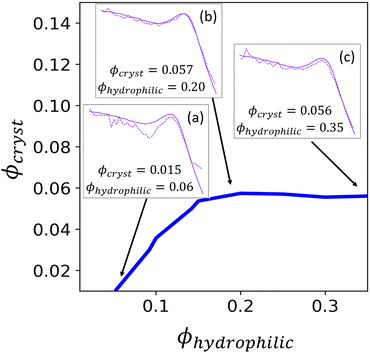
The contour corresponding to the computed experimental Irel of 0.9163 is interpolated from the data in Fig. 7 and is shown in Fig. 9. Any point along this computed contour should give a scattering profile which matches the input experimental scattering profile. However, for smaller hydrophilic and crystallite volume fractions, the match in scattering profile becomes worse (Fig. 9, inset a). Despite the relative peak heights being conserved, both the ionomer peak and matrix knee become narrower than in the experimental profile. At low volume fractions, there is not sufficient volume of each phase within the finite size of our structural reconstruction to fully sample the broad spatial distributions that give rise to the broad ionomer peak and matrix knee. The reconstruction scattering profiles match the experimental profiles at higher hydrophilic and crystallite volume fractions as expected (Fig. 9, insets b and c).
For our final reconstructed structures, we select a volume fraction along the contour corresponding to the Irel in the experimental scattering profile, and with water volume fraction identified from correlations in the previous literature between PFSA polymer design (namely equivalent weight or EW) and water uptake, compiled for a variety of PFSA ionomer materials and conditions in Kusoglu and Weber's review.30 We choose the contour point based on water volume fraction rather than crystalline volume fraction because previous correlations relating EW and crystallinity use wide-angle X-ray scattering (WAXS), which gives only a relative degree of crystallinity, rather than the precise volume fraction.30 If one had access to both relative crystallinity from WAXS measurements as well as water volume fraction from uptake measurements, they could validate that these experimental volume fractions lie on or near the computed contour. These assumptions could be further refined by using scattering data collected at a series of controlled humidities using an environmental chamber. If there is disagreement between the experimentally determined volume fractions and the volume fractions determined using our method, it is likely that the fit function used for deconvolution of the two phases (i.e.eqn (7)) would need to be modified to obtain a better match to the experimentally determined volume fractions.
The above process to identify the optimal crystallite and hydrophilic volume fractions by performing a grid search and defining contours could be replaced by other more sophisticated optimization techniques (genetic algorithms, Bayesian optimization, etc.) that may also improve computational speed. We choose to use the grid search because it demonstrates the degeneracy of our structural reconstruction process i.e., multiple structures may have the same scattering profile with different crystallite and hydrophilic volume fractions. Simultaneously, having a generalized curve enables an informed selection of the volume fractions for the final structural reconstruction based on additional experimental evidence outside of the scattering profile.
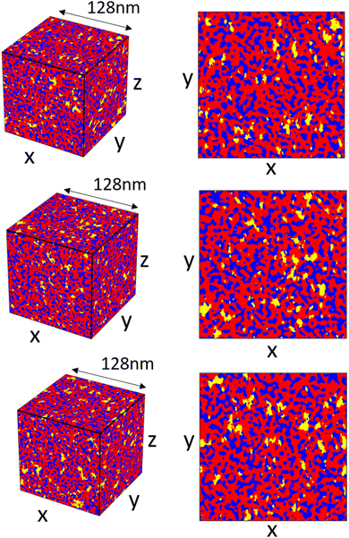
Once the spectral density array has been constructed, generating and combining the random fields to create a final reconstruction are relatively quick (relative times for the different steps are included in Fig. S7, ESI†). We show different reconstructions for the scattering profile, shown in Fig. 2b, in Fig. 10 to demonstrate the variance between different reconstructions using this method. The reconstructions are visually similar with differences in the random shapes and positions of the hydrophilic domains and crystalline domains. Looking at the xy-slices of the structure in Fig. 10b, the crystalline domains show anisotropy, generally being slightly longer in the y-direction; any anisotropy in the hydrophilic domains is not immediately apparent.
By the way in which we have formulated this method, the scattering of the reconstruction should closely match the input scattering, but there are a couple reasons why this might not always be the case. First, low volume fractions for the phases of interest could be insufficient to accurately recreate the scattering. This can be seen, for example in Fig. 9a. Second, because we are combining two separate random fields, it is possible that one interferes with the pattern of the other, which would affect the resulting scattering. We perform a final check to confirm that neither of these reasons is a cause for concern, and that the computed scattering from the reconstruction matches the input experimental scattering. The comparison between the 2D computed scattering profile (Fig. 11a) and the input 2D experimental scattering profile (Fig. 11b) shows good visual agreement. In Fig. 11c, we confirm this match more quantitatively, with a comparison of the 1D scattering profiles along different azimuthal angles of the 2D scattering profiles shown in Fig. 10a and b.
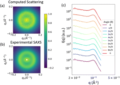 | ||
| Fig. 11 (a) 2D scattering profile computed from reconstructions like those in Fig. 10. (b) input experimental 2D scattering profile. The colorbar denotes log(I(q)) after both profiles have been normalized (c) 1D scattering profiles along different angles of the 2D scattering profiles. Dashed lines indicate the scattering computed from the 3D real space structural reconstructions, while solid lines indicate the input 2D scattering profile from SAXS measurements. | ||
Conclusion
In this work, we have extended the random field small angle scattering analysis method to reconstruct phase-separated structures consisting of three phases with anisotropy from 2D small angle scattering (SAS) data. The method takes, as input, a 2D scattering profile, and involves deconvolution of SAS peaks by fitting to a functional form and interpolating along different azimuthal angles of the scattering profile to preserve the anisotropy. The spectral density along each azimuthal angle is then computed using Fourier transforms and statistical relations to random fields. These spectral densities are interpolated to form a 3D array, which is used to generate two random fields. One level-cut field corresponds to one phase, a second level-cut field corresponds to a second phase, and the remaining space is attributed to the third phase. These fields are then combined to form a final reconstruction in the form of a 3D array where each array entry has one of three discrete values corresponding to the phase of the material at that spatial position. Reconstructions made using this method can be used for structure visualization, to calculate metrics describing the structure, or to perform simulations to calculate material properties such as diffusion.Within this method, several decisions need to be made depending on SAS data quality and availability. The number and size of the angular slices that are averaged over needs to be determined depending on the level of noise in the SAS data. The volume fraction of one phase needs to be experimentally determined via another experimental technique. Lastly, some additional information about the material structure in the direction parallel to the incident SAS beam is required for an accurate reconstruction. If it is possible to take additional SAS measurements of the material in different orientations, measurements of I(qx, qz) or I(qy, qz) could provide that needed information. If these measurements are not possible, then assumptions can be made based on knowledge about the processing or synthesis technique that gave rise to the structural anisotropy.
We have demonstrated successful use of this method for the reconstruction of NafionTM membranes structures from 2D SAXS data, where the three phases are hydrophilic domains consisting of water, sulfonic acid groups, and counterions, crystalline polymer domains, and amorphous polymer domains. We validate the method by showing that computed scattering profiles of these 3D real space structural reconstructions agrees well with the input experimental data.
One should note some of the limitations and assumptions of our presented method before using this method for analysis of other 2D small angle scattering data. First and foremost, the flexibility of the GRF approach will generally allow for a real-space structural reconstruction of any scattering profile, but this does not mean that the reconstruction is the true representation of the material's structure. This uncertainty is due to the degeneracy of structures that can give rise to the same SAS profile. It is important to validate that the GRF model gives structures similar to expected structures from domain expertise as we have done with comparisons to simulated structures from molecular dynamics in Section S1 (ESI†). Such validation is principally important when using reconstructions to compute transport properties, as SAS measurements include only a material's frequency information and not the phase information that is critical to deciphering connectivity. As a result, any transport properties that are calculated from reconstructions are a direct consequence of the assumption that level-cut GRFs can be used to accurately describe the material structure, and the computed properties are meaningless if this is not the case. Additionally, the method, as presented, assumes two of the phases are independent of one another (in our use case of NafionTM, the hydrophilic domains and the crystalline polymer domains are the two phases assumed to be independent). Possible future work could involve extending this workflow to incorporate phase dependencies through “plurigaussian” random fields,27 which would necessitate additional information to glean the spatial relationships at interfaces between the different phases.
Author contributions
Stephen Kronenberger: conceptualization, methodology, data curation, validation, visualization, writing – original draft, review, and editing. Nitant Gupta: conceptualization, methodology, writing – review and editing. Benjamin Gould: scattering data acquisition, writing – review and editing. Colin Peterson: scattering data acquisition, writing – review and editing. Arthi Jayaraman: funding acquisition, supervision, writing – review and editing.Data availability
Due to legal confidentiality requirements arising from University of Delaware – Chemours contract, neither our implementation of the code nor the raw SAXS data can be provided.Conflicts of interest
This work was funded, in part, by the Chemours Company, producer of NafionTM membranes. Benjamin Gould and Colin Peterson are salaried employees of the Chemours Company.Acknowledgements
SK and AJ acknowledge support from NSF-NRT Computing and Data Science Training for Materials Innovation, Discovery, Analytics program under Grant DGE 2125703 for the fellowship that supported SK. AJ and NG are grateful for financial support from Chemours Company that partially supported NG during this project. This research was supported in part by the Information Technologies resources at the University of Delaware, including use of the Caviness supercomputing cluster.References
- Y. Wei and M. J. A. Hore, J. Appl. Phys., 2021, 129, 171101 CrossRef CAS.
- O. Glatter and O. Kratky, Small Angle X-ray Scattering, Academic Press, London, 1982 Search PubMed.
- A. Guinier, G. Fournet, C. B. Walker and G. H. Vineyard, Phys. Today, 1956, 9, 38–39 CrossRef.
- J. S. Pedersen, Adv. Colloid Interface Sci., 1997, 70, 171–210 CrossRef CAS.
- J. S. Pedersen and P. Schurtenberger, Macromolecules, 1996, 29, 7602–7612 CrossRef CAS.
- F. Nallet, R. Laversanne and D. Roux, J. Phys. II, 1993, 3, 487–502 CrossRef CAS.
- R. Nayuk and K. Huber, Z. Phys. Chem., 2012, 226, 837–854 CrossRef CAS.
- S. V. R. Akepati, N. Gupta and A. Jayaraman, JACS Au, 2024, 4(4), 1570–1582 CrossRef CAS PubMed.
- C. M. Heil, Y. Ma, B. Bharti and A. Jayaraman, JACS Au, 2023, 3, 889–904 CrossRef CAS PubMed.
- C. M. Heil, A. Patil, A. Dhinojwala and A. Jayaraman, ACS Cent. Sci., 2022, 8, 996–1007 CrossRef CAS PubMed.
- Z. Wu and A. Jayaraman, Macromolecules, 2022, 55, 11076–11091 CrossRef CAS.
- Z. Ye, Z. Wu and A. Jayaraman, JACS Au, 2021, 1, 1925–1936 CrossRef CAS PubMed.
- D. Cule and S. Torquato, J. Appl. Phys., 1999, 86, 3428–3437 CrossRef CAS.
- D. Franke and D. I. Svergun, J. Appl. Crystallogr., 2009, 42, 342–346 CrossRef CAS PubMed.
- P. Seibert, A. Raßloff, K. Kalina, M. Ambati and M. Kästner, Int. Mater. Manuf. Innov., 2022, 11, 450–466 CrossRef.
- D. T. Hristopulos, Random Fields for Spatial Data Modeling: A Primer for Scientists and Engineers, Springer Netherlands, Dordrecht, 2020 Search PubMed.
- L. Pantelidis, E. Gravanis and D. V. Griffiths, Engineering Geology for Society and Territory, 2015, vol. 2 Search PubMed.
- L. Théodon, C. Coufort-Saudejaud and J. Debayle, Pattern Recogn., 2024, 149, 110255 CrossRef.
- T. Most and C. Bucher, Prob. Eng. Mech., 2007, 22, 219–229 CrossRef.
- J. L. Starck, K. E. Themelis, N. Jeffrey, A. Peel and F. Lanusse, Astron. Astrophys., 2021, 649, A99 CrossRef CAS.
- R. Bansal, L. H. Staib, D. Xu, H. Zhu and B. S. Peterson, IEEE Trans. Med. Imaging, 2007, 26, 46–57 Search PubMed.
- J. W. Cahn, J. Chem. Phys., 1965, 42, 93–99 CrossRef CAS.
- N. F. Berk, Phys. Rev. A: At., Mol., Opt. Phys., 1991, 44, 5069–5079 CrossRef CAS PubMed.
- N. F. Berk, Phys. Rev. Lett., 1987, 58, 2718–2721 CrossRef CAS PubMed.
- M. Teubner, Europhys. Lett., 1991, 14, 403–408 CrossRef CAS.
- C. J. Gommes and A. P. Roberts, Phys. Rev. E: Stat., Nonlinear, Soft Matter Phys., 2008, 77, 041409 CrossRef PubMed.
- C. J. Gommes, J. Appl. Crystallogr., 2013, 46, 493–504 CrossRef CAS.
- C. J. Gommes, R. Chattot and J. Drnec, J. Appl. Crystallogr., 2020, 53, 811–823 CrossRef CAS PubMed.
- C. J. Gommes, Microporous Mesoporous Mater., 2018, 257, 62–78 CrossRef CAS.
- A. Kusoglu and A. Z. Weber, Chem. Rev., 2017, 117, 987–1104 CrossRef CAS PubMed.
- A. Kusoglu, T. J. Dursch and A. Z. Weber, Adv. Funct. Mater., 2016, 26, 4961–4975 CrossRef CAS.
- K. D. Kreuer, M. Schuster, B. Obliers, O. Diat, U. Traub, A. Fuchs, U. Klock, S. J. Paddison and J. Maier, J. Power Sources, 2008, 178, 499–509 CrossRef CAS.
- J. A. Elliott, D. Wu, S. J. Paddison and R. B. Moore, Soft Matter, 2011, 7, 6820 RSC.
- G. Dorenbos and K. Morohoshi, J. Chem. Phys., 2013, 138, 064902 CrossRef CAS PubMed.
- S.-Y. Choi, M. M. Ikhsan, K. S. Jin and D. Henkensmeier, Int. J. Energy Res., 2022, 46, 11265–11277 CrossRef CAS.
- E. J. Roche, M. Pineri, R. Duplessix and A. M. Levelut, J. Polym. Sci., Polym. Phys. Ed., 1981, 19, 1–11 CrossRef CAS.
- G. Gebel and J. Lambard, Macromolecules, 1997, 30, 7914–7920 CrossRef CAS.
- L. Rubatat, G. Gebel and O. Diat, Macromolecules, 2004, 37, 7772–7783 CrossRef CAS.
- K.-D. Kreuer and G. Portale, Adv. Funct. Mater., 2013, 23, 5390–5397 CrossRef CAS.
- K. Schmidt-Rohr and Q. Chen, Nat. Mater., 2008, 7(1), 75–83 CrossRef CAS PubMed.
- J. J. Madinya, S. Kronenberger, B. Gould, C. Peterson and A. Jayaraman, Macromolecules, 2024, 57(16), 8223–8239 CAS.
- A. Peltonen, J. Etula, J. Seitsonen, P. Engelhardt and T. Laurila, ACS Appl. Polym. Mater., 2021, 3, 1078–1086 CrossRef CAS.
- F. I. Allen, L. R. Comolli, A. Kusoglu, M. A. Modestino, A. M. Minor and A. Z. Weber, ACS Macro Lett., 2015, 4, 1–5 CrossRef CAS PubMed.
- N. V. Aieta, R. J. Stanis, J. L. Horan, M. A. Yandrasits, D. J. Cookson, B. Ingham, M. F. Toney, S. J. Hamrock and A. M. Herring, Macromolecules, 2009, 42, 5774–5780 CrossRef CAS.
- P. Debye and A. M. Bueche, J. Appl. Phys., 1949, 20, 518–525 CrossRef CAS.
- M. Teubner and R. Strey, J. Chem. Phys., 1987, 87, 3195–3200 CrossRef CAS.
- Y. Zhao, K. Yoshimura, T. Motegi, A. Hiroki, A. Radulescu and Y. Maekawa, Macromolecules, 2021, 54, 4128–4135 CrossRef CAS.
- M. Georgiadis, M. Guizar-Sicairos, A. Zwahlen, A. J. Trüssel, O. Bunk, R. Müller and P. Schneider, Bone, 2015, 71, 42–52 CrossRef CAS PubMed.
- Y. Liu, J. Li, S. Sun and B. Yu, Comput. Geosci., 2019, 23, 1011–1047 CrossRef.
- J. Lequieu, J. Chem. Phys., 2023, 158, 244902 CrossRef CAS PubMed.
- S. P. Fernandez Bordín, H. E. Andrada, A. C. Carreras, G. E. Castellano, R. G. Oliveira and V. M. Galván Josa, Polymer, 2018, 155, 58–63 CrossRef.
- K. Schmidt-Rohr, J. Appl. Crystallogr., 2007, 40, 16–25 CrossRef CAS.
- D. P. Olds and P. M. Duxbury, J. Appl. Crystallogr., 2014, 47, 1077–1086 CrossRef CAS.
Footnote |
| † Electronic supplementary information (ESI) available. See DOI: https://doi.org/10.1039/d4sm00721b |
| This journal is © The Royal Society of Chemistry 2024 |

