 Open Access Article
Dissolved oxygen forecasting in the Mississippi River: advanced ensemble machine learning models
Francesco
Granata
 *a,
Senlin
Zhu
 b and
Fabio
Di Nunno
a
aDepartment of Civil and Mechanical Engineering (DICEM), University of Cassino and Southern Lazio, Italy. E-mail: f.granata@unicas.it
bCollege of Hydraulic Science and Engineering, Yangzhou University, Yangzhou, China
First published on 30th July 2024
Abstract
Dissolved oxygen (DO) is an important variable for rivers, which controls many biogeochemical processes within rivers and the survival of aquatic species. Therefore, accurate forecasting of DO is of great importance. This study proposes two models, including AR-RBF by leveraging the additive regression (AR) of radial basis function (RBF) neural networks and MLP-RF by stacking multilayer perceptron (MLP) and random forest (RF), for the prediction of daily DO with multiple forecast horizons (1 day ahead to 15 days ahead) in the Mississippi River using a long-term observed dataset from the Baton Rouge station. Two input scenarios were considered: scenario A includes mean water temperature and a certain number of preceding DO values and scenario B comprises solely the aforementioned number of preceding DO values while entirely disregarding exogenous variables. The AR-RBF and stacked MLP-RF models excel in short-term forecasting and offer sufficiently accurate predictions for medium-term horizons of up to 15 days. For instance, in 3 day ahead predictions, the root mean square error (RMSE) amounts to 0.28 mg L−1, with the mean absolute percentage error (MAPE) hovering around 2.5% in the worst-case scenario. Similarly, for 15 day ahead forecasts, RMSE remains below 0.93 mg L−1, with MAPE not exceeding 8.2%, even under the worst-case scenario. Both models effectively capture the extreme values and the fluctuations of DO. However, as the forecasting horizon is extended, both models experience a decrease in accuracy, which is particularly evident for scenario B when the average water temperature is not included in the input variables. When examining longer forecasting horizons in the study, AR-RBF demonstrates a more restrained bias as compared to the stacked MLP-RF model. The consistently robust performance of the models, in comparison to prior research on DO levels in US rivers, underscores their potential as more effective tools for predicting such an essential water quality parameter.
Environmental significanceProblem/situation: Mississippi River's fluctuating dissolved oxygen (DO) levels affect aquatic ecosystems and biogeochemical processes. Why is it important to address/understand this? Accurate DO forecasting is vital for ecosystem health, aquatic species survival, and effective river management. Key finding and implications: our study introduces two DO prediction models, AR-RBF and MLP-RF. Scenario A, considering water temperature and past DO values, significantly enhances forecast accuracy over scenario B. This emphasizes the need to integrate environmental factors for better river conservation and management. These models offer promising tools for sustainable river ecosystem management. |
1. Introduction
The degradation of surface and groundwater resources is a matter of great concern on a global scale. In particular, development and population growth are accelerating the exploitation of water resources as well as enhancing their deterioration.From this perspective, among the different water quality (WQ) parameters, dissolved oxygen (DO) is a critical indicator, playing a key role in maintaining the proper functioning of aquatic ecosystems.1 There are several factors affecting DO, including temperature and atmospheric pressure, as well as anthropic factors. Furthermore, the water absorption capacity of the oxygen and the DO fluctuations are significantly affected by the environment. In particular, the absorption capacity of water to oxygen is lower on rainy days, whereas DO fluctuations are smaller on sunny and windy days.2 Over the past few decades, researchers have extensively studied the intricate and non-linear dynamics of DO3 to accurately quantify and predict dissolved oxygen levels based on hydrological, meteorological, and water quality parameters.
These predictions can be conducted using different approaches. Among these, physically-based models produce deterministic equations derived from the fundamental laws of physics, such as the conservation laws. These models simulate the biotic and abiotic processes governing the environmental system under study. Despite their robustness, physically-based models are generally time and cost-consuming due to the complexity of these processes and the extensive data requirements for calibration and validation. The inherent complexities of biotic interactions and abiotic conditions often cannot be fully captured, resulting in limitations in their practical applicability.4
In contrast, statistical models, which are grounded in historical data, identify patterns and relationships between input and output variables. While these models are less resource-intensive and faster to implement, they usually lack accuracy due to several factors, including natural data noise, incomplete data, and limited spatial resolution.5 Additionally, statistical models are typically constrained by the assumptions of linearity and normality, which may not adequately represent the non-linear and dynamic nature of environmental processes.
To overcome the high uncertainty and complexity associated with environmental and hydrological processes, researchers have increasingly adopted data-driven approaches in recent years. Among these, artificial intelligence (AI) algorithms, particularly machine learning (ML) and deep learning (DL) methods, have gained prominence. These approaches do not require explicit definitions of the relationships between input and target variables, allowing for fast processing and the ability to handle complex, non-linear interactions within the data.6 Specifically, ML and DL algorithms can be employed individually or in ensemble forms, combining multiple models to enhance forecasting performance.7–9
Recent studies have extensively explored the use of ML models for predicting DO levels in various aquatic environments. Asadollahfardi et al.10 explored the modelling of DO in the Amir Kabir reservoir in Iran using artificial neural networks. This study demonstrated the applicability of neural networks in predicting DO levels in reservoirs, emphasizing the potential of AI methods in various aquatic environments. Abba et al.11 employed four different AI-based models, namely, the long short-term memory neural network (LSTM), extreme learning machine (ELM), Hammerstein–Wiener (HW), and general regression neural network (GRNN), for predicting DO concentrations in the Kinta River, Malaysia, using water quality parameters as inputs. They further developed ensemble models combining these individual models, with the HW-RF ensemble model demonstrating the best predictive skill. While this study highlighted the potential of ensemble models in improving prediction accuracy, it primarily focused on combining multiple simple models without addressing the complexity of dynamic environmental interactions. Building on this, Chen et al.12 developed a hybrid model incorporating an attention mechanism (AT) with LSTM to predict DO levels in the Burnett River, Australia. Including AT significantly enhanced the LSTM model's prediction performance by focusing on relevant parts of the input data. However, this approach still faced challenges in dealing with large-scale datasets and diverse environmental conditions. Maroufpoor et al.13 introduced various neuro-fuzzy (NF) hybrid models, including NF with grey wolf optimizer (NF-GWO), subtractive clustering (NF-SC), and c-mean (NF-FCM), for predicting DO in California rivers. They identified that the NF-GWO model with all variables as input provided the best performance. This study addressed the challenge of optimizing input variable combinations, but the models' generalizability to other regions with different environmental conditions remained limited. Huan et al.14 tackled the issue of missing data by using a random forest (RF) model for data interpolation before applying various ML models, such as the adaptive neuro fuzzy inference system (ANFIS) and radial basis function-artificial neural network (RBF-ANN), for multi-step ahead DO predictions in the Jiangnan Canal, China. Their results showed that the attention-based GRU model outperformed all other models. However, the interpolation of missing data introduced additional uncertainty, and the study did not fully explore the impact of exogenous factors. Li et al.15 addressed the problem of selecting optimal input parameters by applying principal component analysis (PCA) before using a hybrid model of improved particle swarm optimization (IPSO) and least squares support vector machine (LSSVM) for DO prediction in the Yangtze River Estuary, China. They identified eight key parameters that significantly influenced DO levels, thus refining the input selection process. Despite this, the model's performance in scenarios with limited data or varying temporal scales was not thoroughly investigated.
These studies collectively advance the understanding of ML applications in DO prediction by addressing various challenges, such as model complexity, input optimization, handling temporal dependencies, and managing missing data. However, several limitations persist: the primary limitation being the restricted ability of existing models to achieve highly accurate forecasts for extended horizons (beyond 7 days) while considering only the mean water temperature as the sole exogenous variable. This limitation highlights the need for models that can enhance prediction accuracy across various extended forecasting horizons and handle varying data quality and availability.
This study aims to address these gaps by evaluating the effectiveness of a pioneering predictive model, leveraging the additive regression of radial basis function neural networks (AR-RBF), in generating accurate short-term (1–3 days) and medium-term (7–15 days) forecasts of DO concentrations in the Mississippi River, including regular values, high peaks, and low peaks (potentially causing hypoxic or anoxic conditions, stressing or killing aquatic organisms, and disrupting ecosystem health and biodiversity). It is worth noting that the low or high levels of DO issues in the Mississippi Delta plain have been widely investigated in the literature.16,17 However, the implementation of predictive models focused on the prediction of the DO in the Mississippi River is relatively rare to date.18
To the best of the authors' knowledge, herein, the AR-RBF algorithm is employed for the first time to address a water quality forecasting problem. This investigation seeks to assess the AR-RBF model's predictive capability and compare it rigorously with a well-established predictive framework renowned for its accuracy: the MLP-RF stacked model integrating elastic net as a meta-learner.
By analyzing the performance of these models, the study aims to provide comprehensive insights into their respective merits and limitations in predicting dissolved oxygen levels. Such insights are crucial for enhancing our understanding of predictive modelling techniques designed for environmental monitoring and management within river ecosystems.
Predictive models capable of providing reliable forecasts empower decision-makers with timely information to implement proactive measures for monitoring and mitigating potential oxygen deficits or surpluses. In the context of major rivers like the Mississippi, which hold significant ecological and economic importance, precise forecasts enable stakeholders to anticipate fluctuations in DO levels. This information is invaluable for informing adaptive management strategies and supporting sustainable resource management practices. The utilization of advanced predictive modelling techniques, such as the AR-RBF model and the MLP-RF stacked model, holds promise for enhancing the accuracy and timeliness of DO forecasts. By harnessing the capabilities of these models, environmental authorities and stakeholders can proactively address emerging challenges, optimize resource allocation, and ultimately foster the preservation and restoration of riverine ecosystems. Thus, the outcomes of this investigation advance not only scientific knowledge but also offer practical benefits for environmental management and sustainability efforts in river ecosystems, underscoring the significance of robust predictive modelling in contemporary environmental managing practices.
2. Materials and methods
2.1 Additive regression of radial basis function neural network
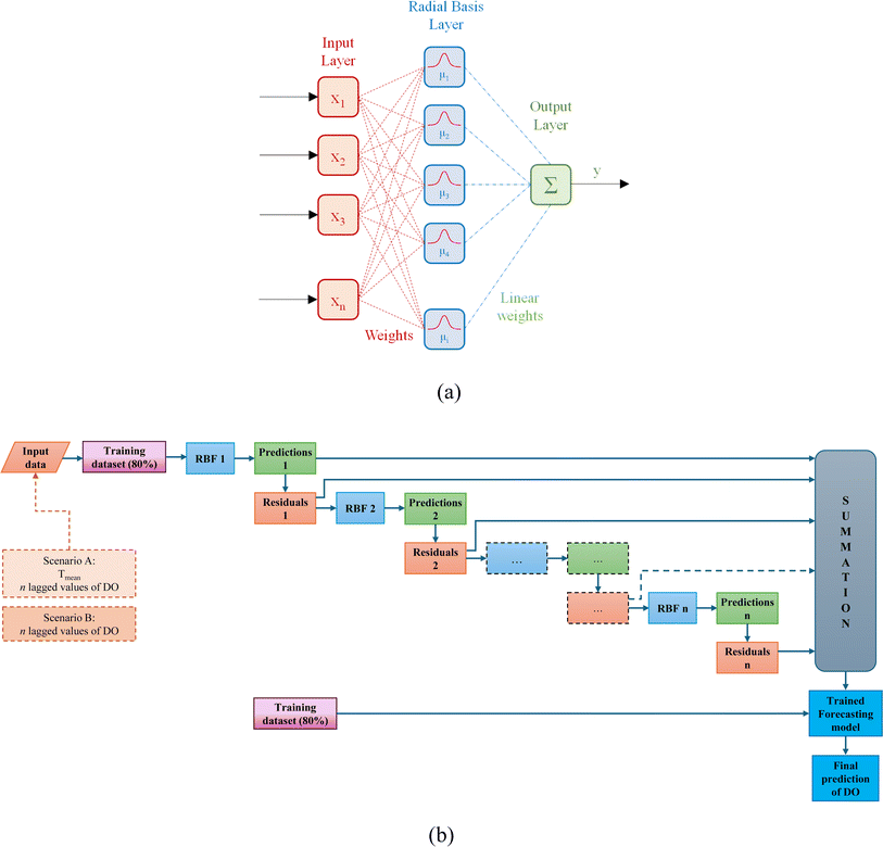
Additive regression, an ensemble learning technique, acts as an advanced metaclassifier, significantly boosting the predictive capability of basic regression models.19 It presents a novel approach to predicting DO levels in hydrological systems. Employing an iterative procedure, each model is adjusted to the residuals left by its predecessor, leading to a gradual refinement of predictions. Ultimately, the final prediction is derived from the aggregation of outputs from individual classifiers (Fig. 1b). The incorporation of a shrinkage parameter plays a crucial role in preventing overfitting and introducing a smoothing effect. However, it is important to note that reducing the shrinkage parameter may result in longer learning times. Despite its potential, additive regression remains relatively underexplored in predictive hydrological modelling, with tree models being more commonly used in existing literature.20In this study, the radial basis function neural network (RBF-NN) algorithm was selected as the base regressor. The RBF-NN architecture consists of three layers: an input layer, a hidden layer, and an output layer. The operation of the hidden layer involves employing radial basis functions to transform input data into a higher-dimensional space, thereby simplifying the regression task. Radial basis functions, mathematical constructs centered at specific points, exhibit exponential decay as the distance from the center increases. The initial centers for Gaussian radial basis functions are determined using the K-means algorithm. Among the various activation functions available for the hidden layer, the Gaussian function is commonly adopted. Typically, the output layer of the RBF neural network combines activations from the hidden layer linearly (Fig. 1a). The weights for this combination are determined through either a least-squares approach or gradient descent optimization.
A notable advantage of the RBF-NN lies in its reduced dependence on extensive training data compared to alternative neural network architectures. This is attributed to the capability of the hidden layer to extract features effectively, thereby reducing the dimensionality of the input data. Additionally, the RBF-NN demonstrates enhanced resilience to overfitting, making it an attractive option for various modelling tasks.21
2.2 Stacked model of multilayer perceptron and random forest
Other valuable ensemble models can be obtained using the stacking methodology; this typically comprises multiple layers. In the initial layer, diverse base models employing different algorithms are developed using the training dataset. The outputs of these base models serve as input features for the subsequent layer, which acts as the meta-learner, integrating outputs from the base models to formulate the final prediction. The stacked ensemble model utilized in this research incorporates the multilayer perceptron (MLP) and random forest (RF) algorithms as base models, with the elastic net (EN) algorithm selected as the meta-learner (Fig. 2c).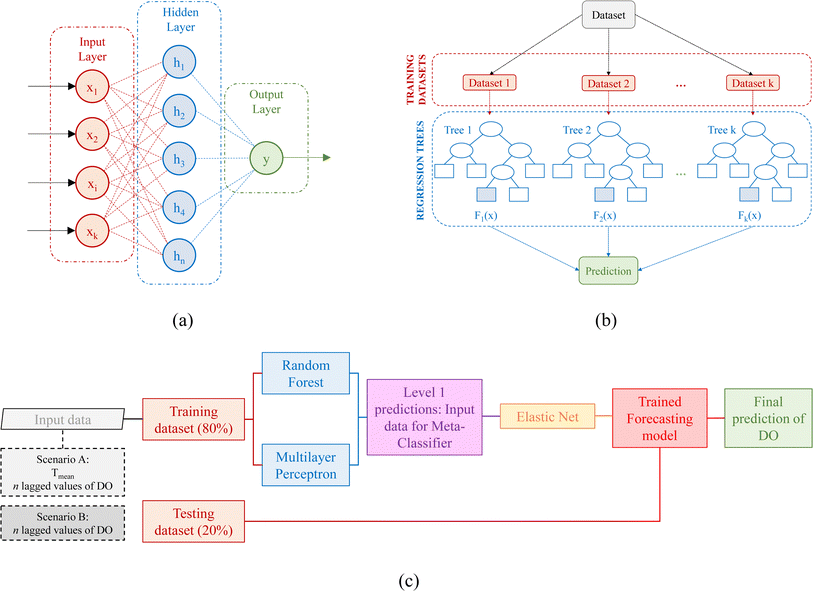 | ||
| Fig. 2 Schemes related to multilayer perceptron (a), random forest (b), and the architecture of the stacked procedure (c). | ||
The MLP is a type of feedforward neural network characterized by its stratified architecture.22 It encompasses an input layer, one or more hidden layers, and an output layer. Each layer comprises interconnected neurons, with data flowing uniquely in a unidirectional manner, from input to output (Fig. 2a). The initial layer of the MLP receives input data, typically presented as feature vectors. Each neuron within this layer corresponds to a specific feature of the input data. The MLP may embody one or multiple hidden layers, tasked with hierarchical feature extraction and abstract representation learning. Neurons within the hidden and output layers calculate a weighted summation of inputs, followed by the application of an activation function, which introduces non-linearity, facilitating the network's ability to discern intricate patterns. The connections between neurons in consecutive layers are associated with trainable parameters termed weights. Each neuron usually has a bias term, contributing to the overall transformation. The weights and biases are typically initialized randomly at the outset of training and adjusted iteratively during the optimization process. Common activation functions include sigmoid, rectified linear unit (ReLU), and hyperbolic tangent, each offering distinct characteristics influencing the network's performance and training velocity. The final layer of the MLP generates the ultimate predictions or representations of the input data, contingent on the task at hand. MLPs learn by minimizing a loss function quantifying the disparity between predicted and actual outputs. The backpropagation algorithm iteratively updates the weights based on the gradients of the loss function, thereby enhancing the model's performance. Conventional optimization techniques such as stochastic gradient descent (SGD) or its variants are employed to optimize the network's weights and biases. Training data is often partitioned into batches to enhance computational efficiency during optimization.
Random forest (RF), introduced by Breiman,23 represents an ensemble learning technique comprising multiple regression trees, where each tree is independently constructed and contributes to the final prediction through averaging. The fundamental components of an RF are regression trees, which partition the input data space into segments based on feature values to formulate predictions (Fig. 2b). RF employs a bagging approach, randomly sampling the training data with replacement to generate multiple datasets for each decision tree, thereby promoting diversity and robustness. During the construction of each regression tree, a random subset of features is considered at each split, mitigating the risk of overfitting and bolstering generalization. The regression trees are recursively grown by selecting the optimal feature and split point at each node, based on mean squared error. RFs frequently impose a maximum depth restriction on the trees to forestall excessively deep trees and potential overfitting. RFs strike a balance between variance reduction (through prediction averaging) and bias control (via multiple regression trees). Furthermore, amalgamating numerous regression trees further mitigates the risk of overfitting and enhances RFs' resilience to noisy data. RFs demonstrate efficacy on high-dimensional and large-scale datasets, showcasing robust generalization capabilities.
The elastic net algorithm24 is a versatile regression method that combines the strengths of lasso and ridge regression. Unlike lasso, which tends to select only one variable from a group of correlated predictors, and ridge regression, which doesn't perform feature selection, the elastic net method strikes a balance between the two.
At its core, the elastic net algorithm aims to minimize the loss function by adding a regularization term that penalizes the size of the coefficients. This regularization term consists of a combination of L1 and L2 penalties. The L1 penalty encourages sparsity by shrinking some coefficients to zero, promoting feature selection. Meanwhile, the L2 penalty encourages smaller coefficients overall, helping to prevent overfitting.
By adjusting the hyperparameter alpha, users can control the relative influence of the L1 and L2 penalties. A higher alpha value emphasizes the L1 penalty, favoring sparsity and feature selection, while a lower alpha value emphasizes the L2 penalty, encouraging smaller coefficients overall.
One of the key advantages of the elastic net algorithm is its ability to handle datasets with a large number of features, especially when some of these features are correlated. It effectively addresses the limitations of both lasso and ridge regression, making it a valuable tool in regression analysis, particularly in high-dimensional data settings.
2.3 Case study and dataset
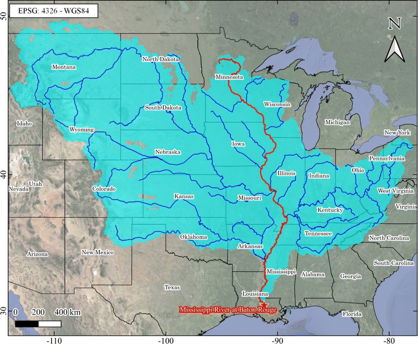
Stretching approximately 3766 km from its source at Lake Itasca in Minnesota to its mouth at the Gulf of Mexico, the Mississippi River (Fig. 3) is one of the most important rivers in North America. Throughout its course, the Mississippi River serves as a vital lifeline for countless communities, ecosystems, and industries. It has played a central role in shaping the cultural, economic, and environmental landscape of the United States. The Mississippi River basin, encompassing 31 U.S. states and two Canadian provinces, drains approximately 40% of the continental United States. Its catchment area spans 3.24 million km2, ranking it as the third-largest drainage basin globally and seventh in terms of both streamflow and sediment load.25,26 Its vast watershed includes a diverse array of landscapes, from the forested regions of the Upper Mississippi to the fertile agricultural plains of the Midwest, and finally to the expansive deltaic wetlands of the Mississippi River Delta.The Mississippi River basin spans a vast area across the central United States, encompassing a wide range of climatic zones. The northern region experiences a continental climate with cold winters and warm summers, with varying precipitation and snowfall in winter. Moving to the central region, the climate is characterized by hot summers and cold winters, with moderate and evenly distributed precipitation throughout the year. The southern region, in contrast, features a humid subtropical climate with hot, humid summers and mild winters, receiving significant rainfall and being prone to severe weather, including thunderstorms and hurricanes.
Geologically, the Mississippi River basin is diverse. The upper basin is dominated by glacial and fluvial deposits, with bedrock composed of sedimentary rocks such as limestone, sandstone, and shale. In the central basin, thick sequences of sedimentary rocks, including shale, limestone, and sandstone, were formed in ancient marine environments. The lower basin comprises extensive alluvial deposits from the Mississippi River, including clay, silt, sand, and gravel. These fertile deposits support agriculture and influence the river's hydrology, sediment transport, and nutrient dynamics, which are critical for dissolved oxygen levels.
Ecologically, the Mississippi River and its associated wetlands provide an essential habitat for a rich diversity of plant and animal species. It supports numerous fish species, including economically valuable species such as catfish, bass, and paddlefish. The river and its floodplains also serve as vital stopover points for migratory birds, supporting millions of waterfowl during their annual migrations.27 However, the Mississippi River also faces significant environmental challenges, including water pollution, habitat loss, and the threat of invasive species.
At Baton Rouge (Louisiana state), where the monitoring station is located, the drainage area is equal to about 3.2 million km2. In particular, the daily data related to gage height (gauge), mean discharge (Qmean), mean water temperature (Tmean), pH, and DO, from February 2016 to April 2024 were considered. Table 1 provides the statistics for each variable.
| h gage (m) | Q mean (m3 s−1) | T mean (°C) | pH | DO (mg L−1) | |
|---|---|---|---|---|---|
| Min | 1.27 | 3766.13 | 2.30 | 6.90 | 5.10 |
| Max | 13.58 | 38![[thin space (1/6-em)]](https://www.rsc.org/images/entities/char_2009.gif) 794.02 794.02 |
31.40 | 8.30 | 13.30 |
| Mean | 7.41 | 18![[thin space (1/6-em)]](https://www.rsc.org/images/entities/char_2009.gif) 160.05 160.05 |
18.56 | 7.77 | 8.35 |
| Median | 7.48 | 16![[thin space (1/6-em)]](https://www.rsc.org/images/entities/char_2009.gif) 876.81 876.81 |
18.20 | 7.80 | 8.10 |
| σ | 3.28 | 8637.30 | 8.30 | 0.19 | 1.98 |
| 1st quartile | 4.54 | 10![[thin space (1/6-em)]](https://www.rsc.org/images/entities/char_2009.gif) 958.60 958.60 |
10.80 | 7.70 | 6.50 |
| 3rd quartile | 9.93 | 23![[thin space (1/6-em)]](https://www.rsc.org/images/entities/char_2009.gif) 899.38 899.38 |
27.10 | 7.90 | 10.20 |
| CV | 0.44 | 0.48 | 0.45 | 0.02 | 0.24 |
| Skew | −0.07 | 0.45 | 0.13 | −0.50 | 0.37 |
The correlation matrix (Table 2) reveals that DO exhibits a high correlation, equal to −0.95, solely with the average water temperature.
| DO | h gage | Q mean | T mean | pH | |
|---|---|---|---|---|---|
| DO | 1 | ||||
| h gage | 0.039 | 1 | |||
| Q mean | 0.043 | 0.986 | 1 | ||
| T mean | −0.953 | −0.259 | −0.261 | 1 | |
| pH | 0.170 | −0.637 | −0.632 | 0.012 | 1 |
The study and prediction of DO levels in the terminal stretch of the Mississippi River, particularly in the Baton Rouge area, are essential endeavours due to their ecological significance and the potential impact of anthropogenic activities. The region's diverse aquatic ecosystems warrant meticulous monitoring to assess their health and biodiversity. The dense population and industrialization of the area pose challenges, with discharges from industrial, agricultural, and urban sources potentially affecting water quality. Given the area's susceptibility to hypoxia, driven by factors such as nutrient loading from agriculture and sediment accumulation, forecasting dissolved oxygen levels has become imperative for understanding and managing hypoxic risk. Moreover, the Mississippi River and surrounding waters are vital for commercial and recreational fishing, making it imperative to mitigate the adverse effects of low dissolved oxygen levels on fish populations and the overall aquatic environment.
2.4 Evaluation metrics
The accuracy of the forecast models was assessed using four different evaluation metrics:(1) Coefficient of determination (R2): this is a statistical measure that represents the proportion of the variance in the dependent variable that is explained by the independent variables in a regression model. It ranges from 0 to 1, with higher values indicating a better fit of the model to the data.
 | (1) |

(2) Mean absolute error (MAE): this is a measure of the average absolute difference between predicted and measured values. It is calculated by taking the average of the absolute differences between each predicted value and its corresponding actual value.
 | (2) |
(3) Mean absolute percentage error (MAPE): this is a measure of the average percentage difference between predicted and measured values. It is calculated by taking the average of the absolute percentage differences between each predicted value and its corresponding actual value, expressed as a percentage.
 | (3) |
(4) Root mean squared error (RMSE): this is a measure of the square root of the average squared difference between predicted and measured values. It is calculated by taking the square root of the average of the squared differences between each predicted value and its corresponding actual value.
 | (4) |
2.5 Model development
Given that in the investigated case study Tmean is the sole exogenous variable highly correlated with dissolved oxygen, to assess its predictive significance, two distinct input variable scenarios were considered in the modelling: scenario A, including Tmean and a certain number of preceding DO values, and scenario B, comprising solely the aforementioned number of preceding DO values, while entirely disregarding exogenous variables. Therefore, the predictors include a series of lagged DO values, alongside the DO of the current day and the mean daily temperature, which is the sole exogenous climatic variable considered. Notably, to streamline and expedite model development, lagged temperature values were omitted from the input variables. It is appropriate to point out that despite this omission, the lagged DO values inherently encapsulate information from these temperature readings.The optimal number of lagged values, denoted as n, and the hyperparameters of the models underwent determination via a Bayesian optimization (BO) procedure. Bayesian optimization has emerged as an effective method for optimizing functions presenting challenges in evaluation and entailing significant computational costs. This methodology involves a sequential model-based approach, leveraging a probabilistic model to capture the intricacies of the function under optimization. As new data points surface, the model undergoes progressive refinement through Bayesian inference, assimilating prior knowledge about the function and uncertainties surrounding the model. This algorithm adeptly navigates the exploration–exploitation trade-off within the search space, leading to the discovery of the global optimum with fewer objective function evaluations compared to alternative optimization techniques.
While a detailed procedural exposition is omitted herein for brevity, interested readers can explore pertinent literature for deeper insights.28 In this study, the Root Mean Square Error (RMSE) was designated as the metric to be minimized.
For training the predictive models, 80% of the data was used, while the remaining 20% was used for testing. Preliminary tests showed that this division was optimal for both achieving adequate model training and having a sufficiently long testing period. Before processing, the data underwent normalization.
The multi-step prediction was executed utilizing a hybrid direct-recursive procedure. In this methodology, a distinct model is formulated for each time step to be forecasted. However, each model leverages predictions from preceding time steps as new lagged DO values to predict future DO values. Given the inherent uncertainty of future values during the forecasting process, the previously predicted values serve as a realistic estimate of the actual values.
3. Results
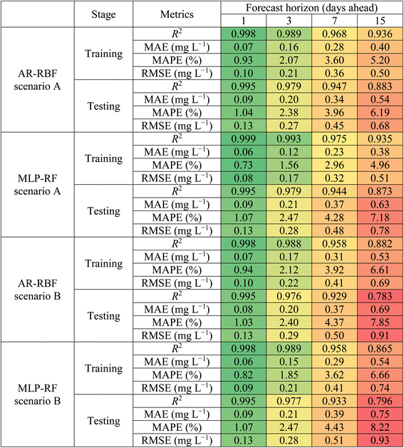
In this section, the performances of the two models (AR-RBF and MLP-RF) were evaluated with different forecast horizons (1 day ahead to 15 days ahead) and input combinations (scenarios A and B). Table 3 presents detailed values of the evaluation metrics considered, with reference to forecast horizons of 1, 3, 7, and 15 days for both the training and testing phases. Conversely, Fig. 4 illustrates the variation of the metrics characterizing the error, specifically focusing on the testing phase, across all forecast horizons ranging from 1 to 15 days.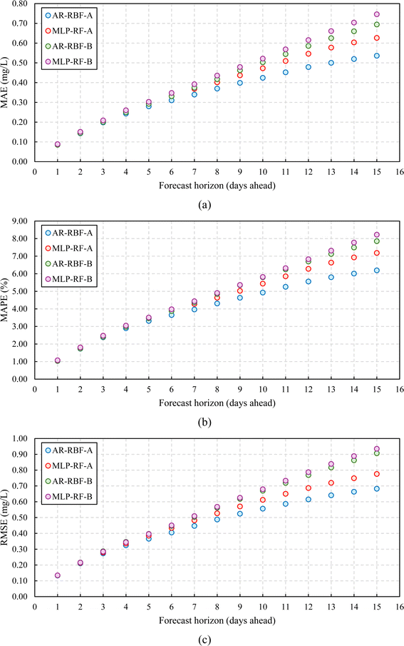 | ||
| Fig. 4 Model performance for scenarios A and B, testing stage, with different forecast horizons: MAE (a); MAPE (b), and RMSE (c). | ||
To ensure a fair and consistent comparison of the different methods, the same training and testing sets were applied across all models evaluated in this study. Specifically, as stated above, 80% of the data was used for training and 20% for testing, maintaining the temporal order of the time-series data to prevent information leakage. Each model was trained and tested using the same data partitions, allowing for a direct comparison of their performance metrics. This consistency ensures that the differences in model performance are attributable to the models themselves and not to variations in the data.
Both the training and testing phases showed that irrespective of the input combination (scenario A or B), both models tended towards deteriorating performance with increasing forecast horizons, as evidenced by increased MAE, MAPE, and RMSE values. However, the best predictions were observed for AR-RBF scenario A that, for the testing stage, showed R2 values between 0.995 (1 day ahead) and 0.883 (15 days ahead). The MLP-RF model in scenario A slightly underperformed the AR-RBF model in scenario A, with R2 values between 0.995 (1 day ahead) and 0.873 (15 days ahead). Scenario B showed a slightly inferior performance, especially at lower forecast horizons. For longer forecast horizons, the gap with scenario A widened. Interestingly, in scenario B, MLP-RF showed slightly higher R2 values and also higher error metrics values than AR-RBF.
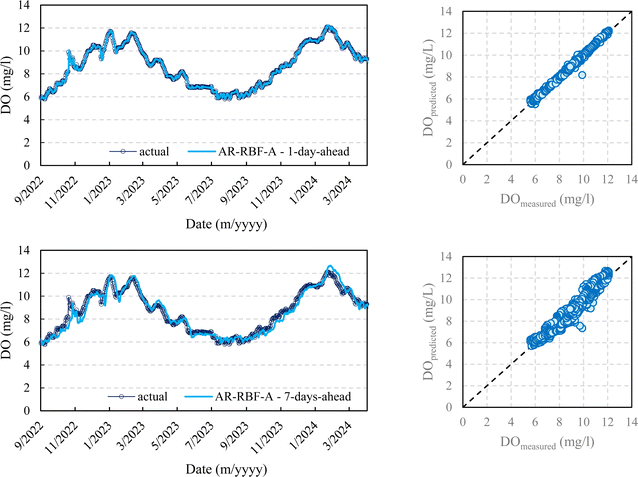
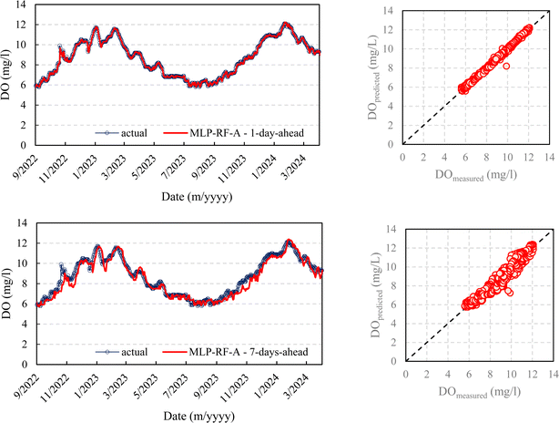
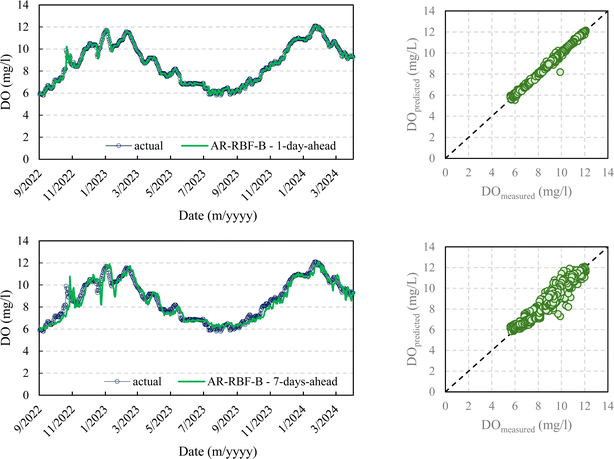
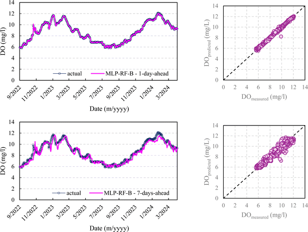
Fig. 5–8 compare the measured and predicted DO during the testing stage for the different models, input combinations, and 1-day ahead and 7-day ahead forecasting horizons.
It seems clear that for the 1-day forecasting horizon, both models, with their two input combinations, demonstrated a high capacity to predict not only the ordinary values of DO but also peaks, maximums, and minimums. Scenarios A and B showed major discrepancies as the forecasting horizon increased. While both AR-RBF and MLP-RF predicted the DO trend with good accuracy, scenario B appeared to be much noisier in its forecasts, with greater oscillations of DO than those present in the testing stage.
Therefore, as the forecasting horizon increases, considering the average temperature as an additional exogenous variable represents a strength in DO prediction.
It must be pointed out that temperature is a key environmental factor influencing water's capacity to hold oxygen; warmer water holds less DO than cooler water. Therefore, changes in average temperature can directly impact DO levels. By incorporating average temperature as an exogenous variable, the models can capture this relationship, enhancing their ability to predict DO fluctuations more accurately. Including temperature provides a more comprehensive view of the environmental conditions affecting DO, making the predictions more reliable and robust across different scenarios and forecasting horizons.
A box plot representation of the relative error evaluated for the testing stage for all models and input combinations is provided in Fig. 9. The relative error was computed as the ratio of the difference between predicted and measured values to the measured values. For a 1 day ahead forecasting horizon, the median values of the relative error were close to 0 for all models and input combinations, with interquartile ranges (IQRs) computed as the difference between the third and first quartile, between 0.014 (AR-RBF scenario B) and 0.0152 (AR-RBF scenario A). As the forecasting horizon increases, the median values become increasingly negative, indicating a more pronounced tendency to underestimate the DO. This trend is more evident for MLP-RF compared to AR-RBF. With AR-RBF, the median values remain closer to zero even for 15-day ahead horizons (−0.009 for AR-RBF scenario A and −0.026 for AR-RBF scenario B).
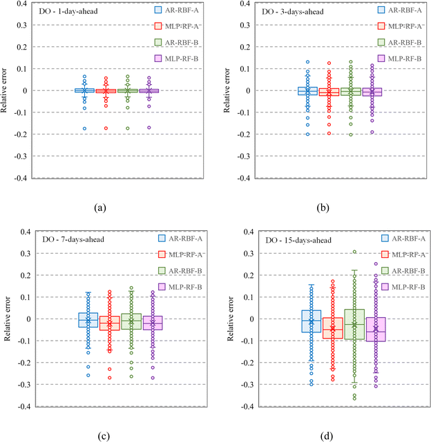 | ||
| Fig. 9 Box plots for scenarios A and B, testing stage, with different forecast horizons: 1 day ahead (a); 3 days ahead (b); 7 days ahead (c); 15 days ahead (d). | ||
For both models and input combinations, an increase in the IQR was observed as the forecasting horizon increased, reaching values between 0.094 (MLP-RF scenario A) and 0.136 (AR-RBF scenario B) for the 15-day ahead prediction. This widening IQR suggests that not only were the median errors shifting (as indicated by becoming increasingly negative) but there was also more dispersion in the prediction errors. In other words, the model's predictions became less consistent with the forecasting horizon increases, reflecting increased uncertainty in long-term forecasts.
Therefore, as the forecasting horizon increases, models can no longer capture the actual variability and dynamics of DO concentrations. This constant underestimation implies that models may not fully account for all the complex factors affecting DO over longer periods, leading to progressively larger prediction errors.
As a consequence, the number of outliers also increased from a few, for the 1-day ahead horizon, to many for the 15-day ahead horizon, highlighting heightened prediction challenges with extended horizons.
4. Discussion
4.1 Impact of forecast horizons and input combinations on model performance
The forecast horizon significantly impacts model performance, which has been well demonstrated in previous studies. For example, Woelmer et al.29 found that the forecast horizon impacts model predictability on near-term phytoplankton forecasts; Di Nunno et al.7 found that with the increase in the forecast horizon, the model tends to perform worse for the forecasting of lake surface water temperatures. The modelling results in the present study showed a reduction in model performance with the increase in the forecast horizon for both models.Typically, the results also indicate that the MLP-RF model is more applicable in the absence of exogenous input variables, while the AR-RBF model exhibited greater performance when including water temperature as an exogenous input. In particular, in this study, water temperature and previous DO values were used as model input to forecast DO considering that water temperature correlated well with DO (correlation coefficient = −0.95), while the other factors like gage height, flow, and pH showed insignificant correlation with DO. The good model performance demonstrated that this choice is appropriate. Previous studies also showed that water temperature is the predominant driver of riverine DO.30–34 For example, Rajesh and Rehana32 showed that water temperature is the main factor impacting DO in Indian rivers, and Zhi et al.33 found that water temperature outweighs light and flow as the primary controller of DO in US rivers. Since water temperature data are more accessible and available compared with other water quality data, the choice of water temperature and previous DO values as model input to forecast DO is very promising. Notably, scenario B, by disregarding exogenous variables like mean water temperature, still works well for short-term forecasts, though the modelling errors are relatively large for medium-term forecasts with large forecast horizons. The results indicate that in regions without enough water temperature measurements, using previous DO values as model input to forecast DO is acceptable, especially for short-term forecasts using the proposed models.
4.2 Modelling performance by comparison with previous studies
Compared with previous ML-based studies on DO modelling in US rivers, the models proposed in this study showed superior performance. For example, Zhi et al.35 employed a DL model to predict DO for US rivers with a mean RMSE of 1.2 mg L−1. As seen in Fig. 4, the RMSE values of the two models for scenario A with different forecast horizons during both the training and testing periods are all below 0.8 mg L−1, lower than that reported by Zhi et al.35 Another example was reported by Moghadam et al.,4 which used a deep recurrent neural network model to model daily DO for Fanno Creek in Oregon, considering three forecast horizons (1 day ahead, 3 days ahead, and 7 days ahead). The RMSE values for 1-day ahead, 3-day ahead, and 7-day ahead predictions by Moghadam et al. (2021) are 0.43 mg L−1, 0.682 mg L−1, and 0.817 mg L−1, respectively. In comparison, the RMSE values in our study are 0.13 mg L−1, 0.28 mg L−1, and 0.46 mg L−1 for scenario A, indicating the better performance of our models. Dumbre et al.18 proposed a polynomial regression model to establish a mathematical link between water temperature and DO for the prediction of DO in the Mississippi River, considering Baton Rouge as a monitoring station, in line with the present study. The authors did not extend the study as the prediction horizon increased. However, for a 1 day ahead prediction, they achieved the R2 value of 0.96, which is good but lower than those found in the present study (R2 = 0.995–0.999).While these comparisons highlight the robustness of the developed models, the authors acknowledge the limitation that the datasets and environmental conditions vary across different studies. Direct comparisons are challenging because the models have been trained and tested on different datasets with varying characteristics. This variability can significantly influence the models' performance and generalizability. To address this limitation and enhance the comparability of DO prediction models, future research should aim to establish standardized datasets that can be used to benchmark different models. Such datasets would allow for a more accurate assessment of model performance across various studies and watersheds, facilitating a better understanding of the strengths and limitations of different modelling approaches.
4.3 Limitations and future developments of the study
The AR-RBF model, concerning short and medium-term DO predictions, has exhibited forecasting capability practically equivalent, or in some cases superior, to that of the stacked MLP-RF model, which had previously demonstrated high performance in hydrological forecasting.6,7,36,37However, it is important to emphasize that the proposed models have been applied to a case study characterized by a limited influence of flow velocity and depth on dissolved oxygen. In the future, the proposed methodology will need to be tested for DO prediction on rivers with different hydrological regimes. Testing the approach on rivers with diverse hydrological features is crucial for its generalizability and robustness. Different rivers may respond differently to predictors, challenging the methodology to adapt and perform under varied conditions. These tests help identify potential weaknesses and biases, refining the approach to enhance the accuracy. Moreover, rivers with diverse characteristics offer broader practical applications, ensuring the global relevance of the methodology. Additionally, rivers flowing through regions with different climates, such as Mediterranean or semi-arid regions, should also be considered. These climates present unique challenges due to varying precipitation patterns, evaporation rates, and water usage practices, which can significantly influence DO levels. From this perspective, incorporating different machine learning or deep-learning algorithms, along with additional exogenous inputs, could enhance the reliability of DO forecasting.
5. Conclusion
Two different prediction models with different input combinations and forecast horizons of up to 15 days were developed for the prediction of the DO in the Mississippi River. The proposed models were obtained by leveraging the AR of RBF neural networks and by stacking MLP and RF. In addition, two input scenarios were considered. The first, scenario A, includes the mean water temperature and the preceding DO values as input, and the second, scenario B, includes only the preceding DO values as input. The key findings can be summarized as follows:- Both the AR-RBF and the stacked MLP-RF models are capable of providing excellent short-term forecasts and sufficiently accurate forecasts for medium-term horizons, up to 15 days. They faithfully reproduce both the extreme values and the fluctuations of DO.
- Both models exhibit a reduction in accuracy as the forecasting horizon is extended. This reduction is more pronounced when the input variables do not include the average water temperature.
- Referring to the longer forecasting horizons considered in the study, AR-RBF exhibits a more limited bias compared to the stacked MLP-RF model.
Overall, the accurate predictions made with both models make them promising tools for proper DO prediction in rivers.
Data availability
The data related to the Mississippi River are available on the USGS website at the following link: https://waterdata.usgs.gov/monitoring-location/07374000.Conflicts of interest
There are no conflicts to declare.References
- A. A. M. Ahmed, S. J. J. Jui and M. A. I. Chowdhury, et al., The development of dissolved oxygen forecast model using hybrid machine learning algorithm with hydro-meteorological variables, Environ. Sci. Pollut. Res., 2023, 30, 7851–7873, DOI:10.1007/s11356-022-22601-z.
- Y. Li, X. Li, C. Xu and X. Tang, Dissolved oxygen prediction model for the Yangtze River Estuary basin using IPSO-LSSVM, Water, 2023, 15(12), 2206, DOI:10.3390/w15122206.
- O. Kisi, M. Alizamir and A. Docheshmeh Gorgij, Dissolved oxygen prediction using a new ensemble method, Environ. Sci. Pollut. Res., 2020, 27, 9589–9603, DOI:10.1007/s11356-019-07574-w.
- S. V. Moghadam, A. Sharafati, H. Feizi, S. M. S. Marjaie, S. B. H. S. Asadollah and D. Motta, An efficient strategy for predicting river dissolved oxygen concentration: application of deep recurrent neural network model, Environ. Monit. Assess., 2021, 193(12), 798, DOI:10.1007/s10661-021-09586-x.
- O. Kisi and M. Cimen, A wavelet-support vector machine conjunction model for monthly streamflow forecasting, J. Hydrol., 2011, 399, 132–140, DOI:10.1016/j.jhydrol.2010.12.041.
- F. Granata, F. Di Nunno and G. de Marinis, Stacked machine learning algorithms and bidirectional Long Short-Term Memory networks for multi-step ahead streamflow forecasting: a comparative study, J. Hydrol., 2022, 613, 128431, DOI:10.1016/j.jhydrol.2022.128431.
- F. Di Nunno, S. Zhu, M. Ptak, M. Sojka and F. Granata, A stacked machine learning model for multi-step ahead prediction of lake surface water temperature, Sci. Total Environ., 2023, 890, 164323, DOI:10.1016/j.scitotenv.2023.164323.
- F. Di Nunno, G. de Marinis and F. Granata, Short-term forecasts of streamflow in the UK based on a novel hybrid artificial intelligence algorithm, Sci. Rep., 2023, 13, 7036, DOI:10.1038/s41598-023-34316-3.
- F. Granata and F. Di Nunno, Neuroforecasting of daily streamflows in the UK for short- and medium-term horizons: a novel insight, J. Hydrol., 2023, 624(2), 129888, DOI:10.1016/j.jhydrol.2023.129888.
- G. Asadollahfardi, S. H. Ariaa and M. Abaeia, Modelling of dissolved oxygen (DO) in a reservoir using artificial neural networks: Amir Kabir Reservoir, Iran, Adv. Environ. Res., 2016, 5(3), 153–167 CrossRef.
- S. I. Abba, N. T. T. Linh, J. Abdullahi, S. I. A. Ali, Q. B. Pham and R. A. Abdulkadir, et al., Hybrid machine learning ensemble techniques for modeling dissolved oxygen concentration, IEEE Access, 2020, 8, 157218–157237, DOI:10.1109/ACCESS.2020.3017743.
- H. Chen, J. Yang and X. Fu, et al., Water quality prediction based on LSTM and attention mechanism: a case study of the Burnett River, Australia, Sustainability, 2022, 14, 13231, DOI:10.3390/su142013231.
- S. Maroufpoor, S. S. Sammen, N. Alansari, S. I. Abba, A. Malik and S. Shahid, et al., A novel hybridized neuro-fuzzy model with an optimal input combination for dissolved oxygen estimation, Front. Environ. Sci., 2022, 10, 929707, DOI:10.3389/fenvs.2022.929707.
- J. Huan, M. Li, X. Xu, H. Zhang, B. Yang and J. Jianming, et al., Multi-step prediction of dissolved oxygen in rivers based on random forest missing value imputation and attention mechanism coupled with recurrent neural network, Water Supply, 2022, 22(5), 5480–5493, DOI:10.2166/ws.2022.154.
- Y. Li, X. Li, C. Xu and X. Tang, Dissolved Oxygen Prediction Model for the Yangtze River Estuary Basin Using IPSO-LSSVM, Water, 2023, 15(12), 2206 CrossRef CAS.
- V. J. Bierman, S. C. Hinz, W. J. Wiseman, N. N. Rabalais and R. Turner, A preliminary mass balance model of primary productivity and dissolved oxygen in the Mississippi River plume/inner Gulf Shelf region, Estuaries, 1994, 17(4), 886–889, DOI:10.2307/1352756.
- B. Dzwonkowski, S. Fournier and J. T. Reager, et al., Tracking sea surface salinity and dissolved oxygen on a river-influenced, seasonally stratified shelf, Mississippi Bight, northern Gulf of Mexico, Cont. Shelf Res., 2018, 169, 25–33, DOI:10.1016/j.csr.2018.09.009.
- A. Dumbre, D. Koli, P. Vaivude and P. Dumbre, Utilizing machine learning within artificial intelligence to enhance dissolved oxygen estimation in the Mississippi River via temperature-driven polynomial regression, Int. J. Res. Appl. Sci. Eng. Technol., 2023, 11(XI), 811–821 CrossRef.
- F. Granata, F. Di Nunno and Q. B. Pham, A novel additive regression model for streamflow forecasting in German rivers, Results Eng., 2024, 22, 102104, DOI:10.1016/j.rineng.2024.102104.
- F. Granata, R. Gargano and G. de Marinis, Artificial intelligence based approaches to evaluate actual evapotranspiration in wetlands, Sci. Total Environ., 2020, 703, 135653, DOI:10.1016/j.scitotenv.2019.135653.
- F. Granata and F. Di Nunno, Forecasting short-and medium-term streamflow using stacked ensemble models and different meta-learners, Stoch. Environ. Res. Risk Assess., 2024, 1–19, DOI:10.1007/s00477-024-02760-w.
- F. Murtagh, Multilayer perceptrons for classification and regression, Neurocomputing, 1991, 2(5–6), 183–197 CrossRef.
- L. Breiman, Random forests, Mach. Learn., 2001, 45, 5–32 CrossRef.
- H. Zou and T. Hastie, Regularization and variable selection via the elastic net, J. R. Stat. Soc. Series B Stat. Methodol., 2005, 67(2), 301–320 CrossRef.
- T. Rosen and Y. J. Xu, Estimation of sedimentation rates in the distributary basin of the Mississippi River, the Atchafalaya River Basin, USA, Hydrol. Res., 2015, 46(2), 244–257, DOI:10.2166/nh.2013.181.
- S. Yin, G. Gao and Y. Li, et al., Long-term trends of streamflow, sediment load and nutrient fluxes from the Mississippi River Basin: impacts of climate change and human activities, J. Hydrol., 2023, 616, 128822, DOI:10.1016/j.jhydrol.2022.128822.
- K. M. Malone, E. B. Webb and D. C. Mengel, et al., Wetland management practices and secretive marsh bird habitat in the Mississippi Flyway: a review, J. Wildl. Manage., 2023, 87, e22451, DOI:10.1002/jwmg.22451.
- J. Snoek, H. Larochelle and R. P. Adams, Practical bayesian optimization of machine learning algorithms, Adv. Neural Inf. Process. Syst., 2012, 25, 1–9 Search PubMed.
- W. M. Woelmer, R. Q. Thomas, M. E. Lofton, R. P. McClure, H. L. Wander and C. C. Carey, Near-term phytoplankton forecasts reveal the effects of model time step and forecast horizon on predictability, Ecol. Appl., 2022, 32(7) DOI:10.1002/eap.2642.
- I. D. Irby, M. A. Friedrichs, F. Da and K. E. Hinson, The competing impacts of climate change and nutrient reductions on dissolved oxygen in Chesapeake Bay, Biogeosciences, 2018, 15(9), 2649–2668, DOI:10.5194/bg-15-2649-2018.
- M. H. Ahmed and L. S. Lin, Dissolved oxygen concentration predictions for running waters with different land use land cover using a quantile regression forest machine learning technique, J. Hydrol., 2021, 597, 126213, DOI:10.1016/j.jhydrol.2021.126213.
- M. Rajesh and S. Rehana, Impact of climate change on river water temperature and dissolved oxygen: indian riverine thermal regimes, Sci. Rep., 2022, 12(1), 9222, DOI:10.1038/s41598-022-12996-7.
- W. Zhi, W. Ouyang, C. Shen and L. Li, Temperature outweighs light and flow as the predominant driver of dissolved oxygen in US rivers, Nat. Water, 2023, 1(3), 249–260, DOI:10.1038/s44221-023-00038-z.
- L. Li, J. L. Knapp, A. Lintern, G. H. C. Ng, J. Perdrial and P. L. Sullivan, et al., River water quality shaped by land–river connectivity in a changing climate, Nat. Clim. Change, 2024, 14(3), 225–237 CrossRef.
- W. Zhi, D. Feng, W. P. Tsai, G. Sterle, A. Harpold and C. Shen, et al., From hydrometeorology to river water quality: can a deep learning model predict dissolved oxygen at the continental scale?, Environ. Sci. Technol., 2021, 55(4), 2357–2368, DOI:10.1021/acs.est.0c06783.
- F. Di Nunno, C. Giudicianni, E. Creaco and F. Granata, Multi-step ahead groundwater level forecasting in Grand Est, France: comparison between stacked machine learning model and radial basis function neural network, Groundw. Sustain. Dev., 2023, 23, 101042, DOI:10.1016/j.gsd.2023.101042.
- M. Lu, Q. Hou, S. Qin, L. Zhou, D. Hua and X. Wang, et al., A stacking ensemble model of various machine learning models for daily runoff forecasting, Water, 2023, 15(7), 1265, DOI:10.3390/w15071265.
| This journal is © The Royal Society of Chemistry 2024 |

