Towards a universal scaling method for predicting equilibrium constants of polyoxometalates

Abstract

The computational prediction of equilibrium constants is still an open problem for a wide variety of relevant chemical systems. In particular, acid dissociation constants (pK_a) are an essential asset in biological, synthetic and industrial chemistry whose prediction encounters several difficulties, requiring the development of novel strategies. The self-assembly of polyoxometalates (POMs) is another complex problem where acid-base reactions play a central role; the successful prediction of the formation constants of these structures is intimately linked with the limitations of pK_a determination. Our methodology POMSimulator enables the prediction of these polyoxometalate formation constants from Density Functional Theory (DFT) calculations, using the experimental K_f values available in the literature to fit the resulting predictions. In this work, we carry out a systematic analysis of a very large number of POM formation constants already predicted through the application of POMSimulator. We then propose a universal scaling scheme for the adjustment of the DFT-based formation constants of POMs, relying on a linear scaling of the form y = mx + b. Here, the slope (m) is a constant parameter – hence, universal towards the nature of the polyoxometalate and the calculation method. The intercept (b), in contrast, is a system-dependent parameter that can be predicted with a multi-linear regression model trained with statistical aggregates of the non-scaled formation constants. Thus, we are able to successfully predict the speciation and phase diagrams of POM systems for which available experimental data are minimal, as well as provide a general scaling scheme that might be extended to other kinds of chemical systems.

---

1 Introduction

Chemical equilibrium is a ubiquitous concept in chemistry. Defined as the point where the rates in both chemical reactions – direct and reverse – are identical,¹ it was first revealed by Berthollet two centuries ago.² Because realistic chemical systems may regard countless simultaneous reactions, it is crucial to utilize computational methods to solve and analyze the resulting systems of coupled chemical equations.³ Current examples are found in a broad range of disciplines: atmospheric chemistry,⁴ chemical oceanography,⁵ electro-chemistry⁶ and geochemistry.⁷

Although equilibrium data are commonly measured from experiments, the steady development of quantum mechanical methods in chemistry has also unlocked the possibility of predicting equilibrium constants.^8–10 However, the main theoretical obstacle is the assessment of the free energy for small solvated ions – in specific, the proton, whose characterization is a centerpiece of acid-base chemistry.¹⁰ The nature of protons in solution has been widely discussed, proposing structures such as the hydronium (H₃O⁺), Zundel (H₅O₂⁺) or Eigen (H₉O₄⁺) cations.^11–15 Choosing a proper proton model is essential for computational chemistry, as the bare H⁺ cation, devoid of electrons, cannot be characterized with ab initio or DFT methods. In the determination of dissociation acid constants (pK_a), a deviation of just 1.36 kcal mol⁻¹ in the reaction free energy leads to an error of one order of magnitude in the resulting constant.¹⁶ To mitigate this issue, there are two main strategies: (i) setting up a thermodynamic cycle in gas and solvent phases and (ii) validating a regression model using experimental data. Relying on these two approaches, it has been possible to predict pK_a values, both in aqueous^17,18 and non-aqueous¹⁹ solvents, below the one logarithmic unit error. The success in predicting equilibrium constants for organic systems is in stark contrast with the scarcer developments in the domain of inorganic chemistry.²⁰ This distinction can be attributed to the highly anionic nature of metallic compounds, which increases the weight of the solvation model in the total free energy. The accuracy of solvation models is a core aspect of computational chemistry and plenty of approaches are available, ranging from implicit, continuum-based models (PCM,^21–23 SMD,²⁴ and COSMO²⁵) to the more costly explicit modeling^26,27 of solvent molecules. Notorious examples of inorganic compounds are polyoxometalates (POMs), which consist of molecular metal-oxo clusters formed by transition metals in high oxidation states linked by oxygen atoms. POMs are pH dependent, with very rich yet complex speciation in solution,^28,29 which represents a limitation for developing novel POM-based technologies in catalysis³⁰ and energy materials.³¹

In our group we have developed a methodology which simulates the aqueous speciation of polyoxometalates from first-principles calculations.³² The methodology has been successfully applied to isopolyoxometalates^33,34 and heteropolyoxometalates.³⁵ Furthermore, we have recently released a polished and open-access version of the source code.^36,37 The workflow of POMSimulator proceeds as follows: once the optimized molecular structures and Gibbs free energies of the building blocks and POMs understudy have been gathered, the methodology starts by automatically generating the chemical reaction network (CRN). Then, the CRN (plus the mass balance equation) is expressed as a complex system of non-linear equations, which leads to an overdetermined system, given that there are more reactions (equations) than compounds (dependent variables). To address this issue, we defined the so-called Speciation Models (SMs), which consist of subsets of chemical reactions that conform to determined solvable systems of equations. The construction of SMs is based on two main hypotheses: (1) all acid-base reactions must be included in the system, due to the importance of pH in the self-assembly processes of POMs and (2) there must be a nucleation reaction for each nuclearity of the molecular set to ensure that all states are accessible.

Solving the SMs delivers the concentrations of all species in the CRNs, which can then be employed to calculate the formation constants for every compound in the network. This procedure ensures that the actual reaction mechanism and pH influence are properly considered in the determination of formation constants. However, these formation constants have proven to be overestimated when compared to experimental values, in line with the pK_a problem mentioned before. In fact, the pK_a issue was also observed when applying POMSimulator to the microkinetic modeling of polyoxotungstates, where the linear scaling of the acid-dissociation constants was crucial to obtain accurate results.³⁸ Furthermore, the fitting between experimental and theoretical pK_a is demonstrated to be dependent on the quantum method of choice.³⁹

Even so, our previous studies showcased some evidence of universality in the scaling parameters. Consequently, in this work we explored this key feature, and we ultimately developed a protocol to streamline the application of POMSimulator to POM systems where only scarce experimental data are available, overcoming previous limitations in the range of applicability of the methodology.

2 Expanding POMSimulator

So far, the application of POMSimulator has relied on conducting a linear scaling between the experimental formation constants reported in the literature and the DFT-based formation constants obtained through this methodology. These formation constants consider the production of a given molecule starting from one or several reference species, usually the monomers, in an acidic medium (eqn (1)). When the heteroatom (X) is not present, as is the case for isopolyoxometalates, r = 0.

Initially, this approach selected the speciation model with the lowest Root Mean Squared Error (RMSE) compared to the reported experimental constants. More recently, we upgraded the methodology by relying on the average scaling parameters (slope, m and intercept, b) of the whole set of SMs, thus making the overall process more robust.

We observed that the slopes of the linear regressions appeared to be constant (≈0.3) across all isopolyoxometalates (Mo, W, V, Nb, and Ta) and heteropolyoxometalates (PMo). In the ESI† we address a minor issue concerning the experimental formation constant of {Mo₃₆}, which at first caused the deviation of the universal slope value. We disregarded the experimental formation constant of {Mo₃₆} for linear scaling, as the leave-one-out methodology identified this constant as an outlier (Fig. S1 and S2†). Considering these pieces of evidence, we sought to study the possible universality of the linear scaling, which would indeed suppose a change of paradigm, practically removing the dependency of POMSimulator on experimental data. In this manner, we would be able to scale DFT-based formation constants without having specific experimental formation constants for a given target system. Combining this with our previously reported statistical pipeline,³⁵ we would be able to explore the speciation and phase diagrams for a much wider set of POM systems for which formation constants might not be available. In this sense, we could invert the way in which POMSimulator is used, by not simply reproducing experimental results, but also releasing new data for guiding further experiments in unknown territory.

2.1 Dependence on the POM system

To further analyze this universality feature, we selected the species for which experimental formation constants were available. We have represented the box-and-whisker plots of the six previously studied systems to characterize the distribution of the computed constants (see Fig. 1). Herein, instead of performing individual regressions for every single speciation model – as in previous studies – we decided to consider the median value for each species as the log(K_DFT) term entering the regression. This does not only reduce the computational cost associated with performing the regressions, but it is also in line with our current statistics-based paradigm, targeting the ensemble of constants instead of individual models. The residuals of the regression are also used to compute error estimates for both m and b, thus defining error bars for the regression line of the form y = (m + σ_m)x + (b + σ_b).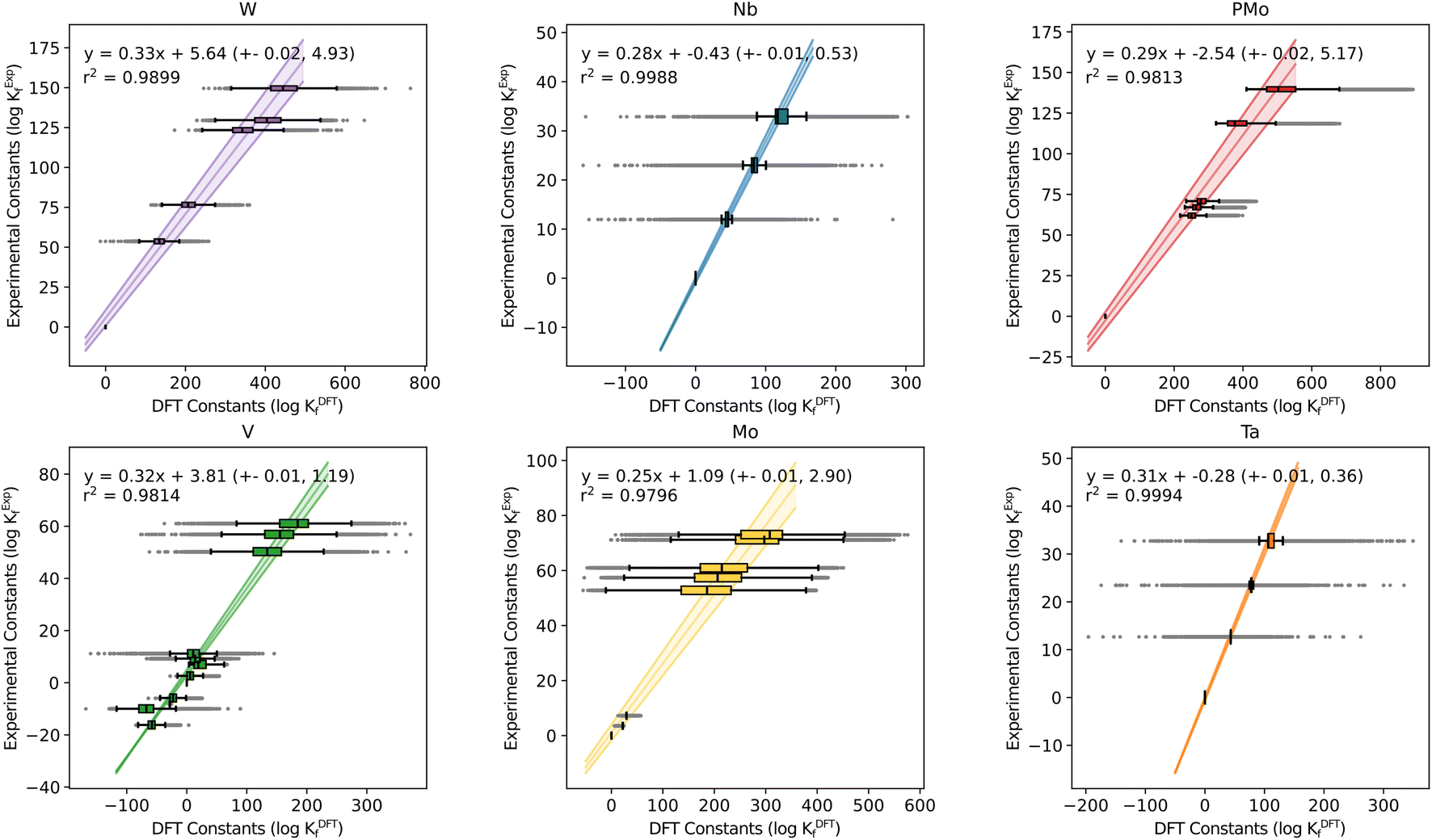

Fig. 1 Box-and-Whisker plot representation for formation constants in Mo, W, V, Nb, Ta and PMo systems, separated by the system. The Y-axis corresponds to experimental values reported in the literature^40–45 and X-axis corresponds to the formation constants predicted with our methodology.

As mentioned before, all the explored systems show very similar slope values, in the range of: 0.25 < m < 0.33. This hints that, regardless of the specific chemical behavior of each POM family, DFT formation constants are overestimated by the same factor in all cases.

Fig. 2 considers a unique regression where all six systems are considered, leading to a single set of linear scaling parameters: m = 0.29 and b = 1.33. As illustrated in Fig. 2, the linear trend is maintained when all compound families are brought together (r² = 0.9635), enabling us to propose a single equation to scale formation constants (eqn (2)).

K_exp = 0.29K_DFT + 1.33 (2)

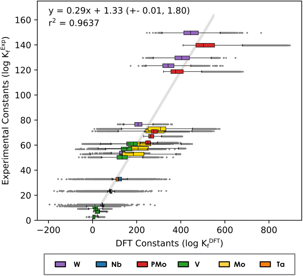Fig. 2 Linear regression of Box-and-Whisker plot representation considering the formation constants in Mo, W, V, Nb, Ta and PMo systems. The Y-axis corresponds to experimental values reported in the literature^40–45 and X-axis corresponds to the formation constants predicted with our methodology.

The error bar estimates show a relatively narrow error band, hinting at the robustness of the approach. Moreover, highlighting the distribution of the constants for each complex demonstrates that for most of the compounds the regression line passes through the central box of the corresponding box plot (that is, the predictions from the linear model are between the 1st and 3rd quartiles).

2.2 Dependence on the DFT functional

Another fundamental question is how the scaling parameters depend on the DFT method used to compute Gibbs free energies. Hitherto, all the systems studied in our group have used the PBE functional. Thus, the values of m and b might be functional-dependent. To explore this effect, we considered all six POM systems that we regarded in previous studies (Mo, W, V, Nb, Ta and PMo) and carried out single-point energy calculations with another GGA functional (BP86), a meta-GGA (M06L) and a hybrid (B3LYP). We calculated the Gibbs free energies by adding the free energy correction term from the PBE results, thus reducing the overall computational cost and adding the electronic energy contribution from a second functional (func) as described here: G(func) = E(func) + ΔG_corr(PBE). Then, we employed POMSimulator to determine the formation constants of the six systems with each of the three new functionals, in order to compare them with the experimentally reported values. Regression lines collating all systems together for the four methods are depicted in Fig. 3: boxplot representations-analogous to Fig. 1 and 2- are shown in Fig. S3.†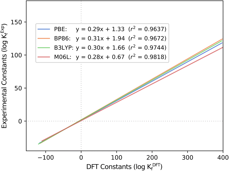

Fig. 3 Regression lines for computed and experimental formation constants extracted from the literature^40–45 throughout the four tested functionals: PBE, BP86, B3LYP and M06L.

The most striking aspect arising from this analysis is, again, the consistency of the slopes for all the regressions, only ranging from m = 0.28 (M06L) to m = 0.31 (BP86). Independent of the functional, the overestimation of the DFT formation constants is approximately the same. This finding hints again at a certain degree of universality in our approach. Furthermore, it also reduces the relevance of functional choice, enabling us to proceed with less computationally demanding calculations (such as PBE) instead of having to resort to more expensive hybrid functionals. This aspect is especially relevant when using the ADF software.⁴⁶ The latter uses Slater-type Orbital (STO) fit functions to speed up the calculation of one-center integrals for GGA,⁴⁷ but it performs significantly slower for exact exchange functionals such as Hybrids.

2.3 Validation with an AsMo system

To validate the adequacy of these universal scaling factors, we decided to test them against a new heteropolyoxometalate, aiming to characterize the speciation from the constants scaled by applying eqn (2). As a target system, we selected arsenomolybdates (AsMo), reported by Pettersson,⁴⁸ for which both speciation diagrams at different Mo : As ratios, as well as formation constants, were available. Having a set of experimental formation constants also enabled us to compute the actual scaling parameters of the AsMo system, to compare them with the predicted values. From these previous studies, we generated the corresponding molecular set, composed of 44 metal-oxo compounds, including key species in arsenomolybdate chemistry, such as the {As₂Mo₆} cluster, which does not form in the analogous PMo system. It is also remarkable that key species for PMo, like the Keggin {PMo₁₂} and lacunary {PMo₁₁} anions, are not reported for AsMo, and therefore were omitted from the molecular set for simplicity. Then, we followed the same protocol as that in our study for phosphomolybdates,³⁵ selecting a random sample on the large set of speciation models produced from the chemical reaction network and computing the formation constants. We applied the scaling equation (eqn (2)) to adjust the formation constants, and then we used them to calculate the speciation diagram of every model. Next, we employed the statistical pipeline to group similar models and select the most adequate average speciation diagrams.

The initial results on the speciation of arsenomolybdates were very poor, as a large fraction of the obtained diagrams only showcased the protonation of arsenates and molybdates, with minimal nucleation (Fig. S4†). Moreover, none of the groups showed any evidence of the major species proposed by Pettersson: {AsMo₉} and {As₂Mo₆}, depending on ratios. To deduce the reason behind these poor results, we determined the specific scaling parameters for the AsMo system from the available experimental constants (see Fig. 4).

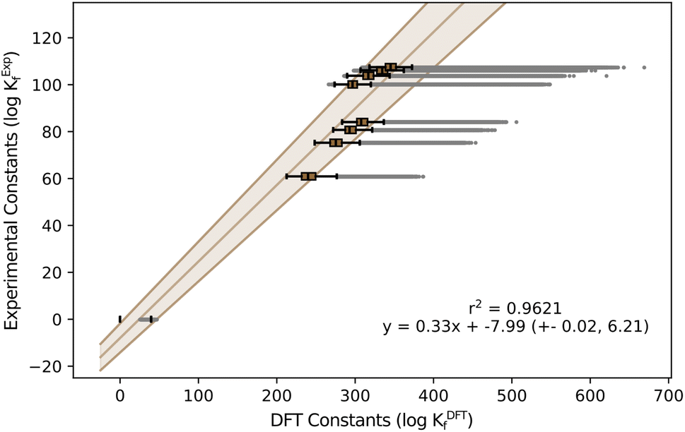Fig. 4 Box-and-Whisker plot representation for formation constants in AsMo. The Y-axis corresponds to experimental values reported in the literature⁴⁸ and X-axis corresponds to the formation constants predicted with our methodology.

While m is consistent with the one obtained in the general regression, Fig. 2, and with the variability observed across systems, Fig. 1, the value of b is inaccurate.

The universal scaling predicts a positive term of b = 1.33, while the actual value for arsenomolybdates is negative b = −7.99. Although a deviation of nine units may not seem concerning, the fact that the intercept is in logarithmic units has a critical effect. In particular, small formation constants are strongly influenced by the intercept, as it contributes more significantly to the scaling than the slope. According to the standard convention for formation reactions, non-scaled formation constants for monomers are either zero (for the non-protonated reference) or close to zero, making them highly sensitive to changes in the intercept. Consequently, the substantial negative shift in the intercept, b = −7.99, is expected to result in smaller formation constants for the monomers, indicating reduced thermodynamic stability. Consequently, employing the universal scaling equation with a positive intercept artificially stabilizes these same monomers, explaining the poor agreement between the simulated speciation and the experimental results.

Considering these findings and revisiting the disparity between the b values determined for each metal system in Fig. 1, the universality precept for the slope does not seem applicable to the intercept. Thus, another strategy is required to actually be able to successfully apply POMSimulator to systems lacking experimental formation constants. While we may still use a constant slope value, there should be a protocol capable of predicting the system-dependent intercepts without resorting to experimental data – hence, only using information derived from the application of our method. We hypothesized that relying on the non-scaled formation constants would serve as the actual input for determining the value of the intercept. Considering the availability of the formation constants for our six initial systems and the AsMo under validation, we collected a set of simple system-wide statistical descriptors across all models, namely: mean, standard deviation, median, quartiles, maximum, minimum, and min–max range. The median value through all species was computed for every descriptor, obtaining a single set of features for every system. From these values, we aimed to identify linear relationships between different feature combinations and the target intercept (Fig. 5).

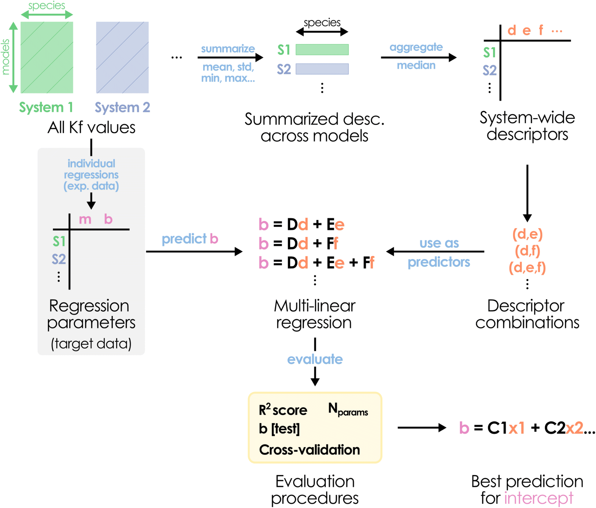Fig. 5 Schematic depiction of the proposed multi-linear regression protocol for predicting the scaling intercept b_AsMo value.

It is important to note that, due to the small number of data points (seven IPA/HPA systems), we should be extremely cautious with the overfitting, especially when considering multiple features at once. Consequently, the evaluation stage is particularly important to determine if a good-performing regression model can provide any kind of generalization. Initially, the AsMo system was employed as a test set, leaving the other six as the training set. Thus, we proceeded to evaluate all regression models in terms of the quality in the prediction of b_AsMo. The ten best MLR models, according to the quality of the prediction of the target intercept, are collected in the ESI (Table S1).† We selected the two well-performing combinations with only three features, corresponding to (Q₃, max, range) and (mean, max, range), with the goal of minimizing the number of required descriptors. Both of them show reasonable r² scores (0.967 and 0.948) and good predictions of b_AsMo (−7.29 and −8.72, respectively). Considering our limitations in terms of acquiring more data (which would require full characterization of molecular sets, application of POMSimulator, and availability of experimental data to perform scalings), we followed with a cross-validation strategy, applying a leave-two-out approach. In this way, for every feature combination we select a two-system validation set, with the other five (including AsMo) being used for training, and then explore the distribution of the obtained predictions. A heatmap representation of these results is showcased in Fig. 6.

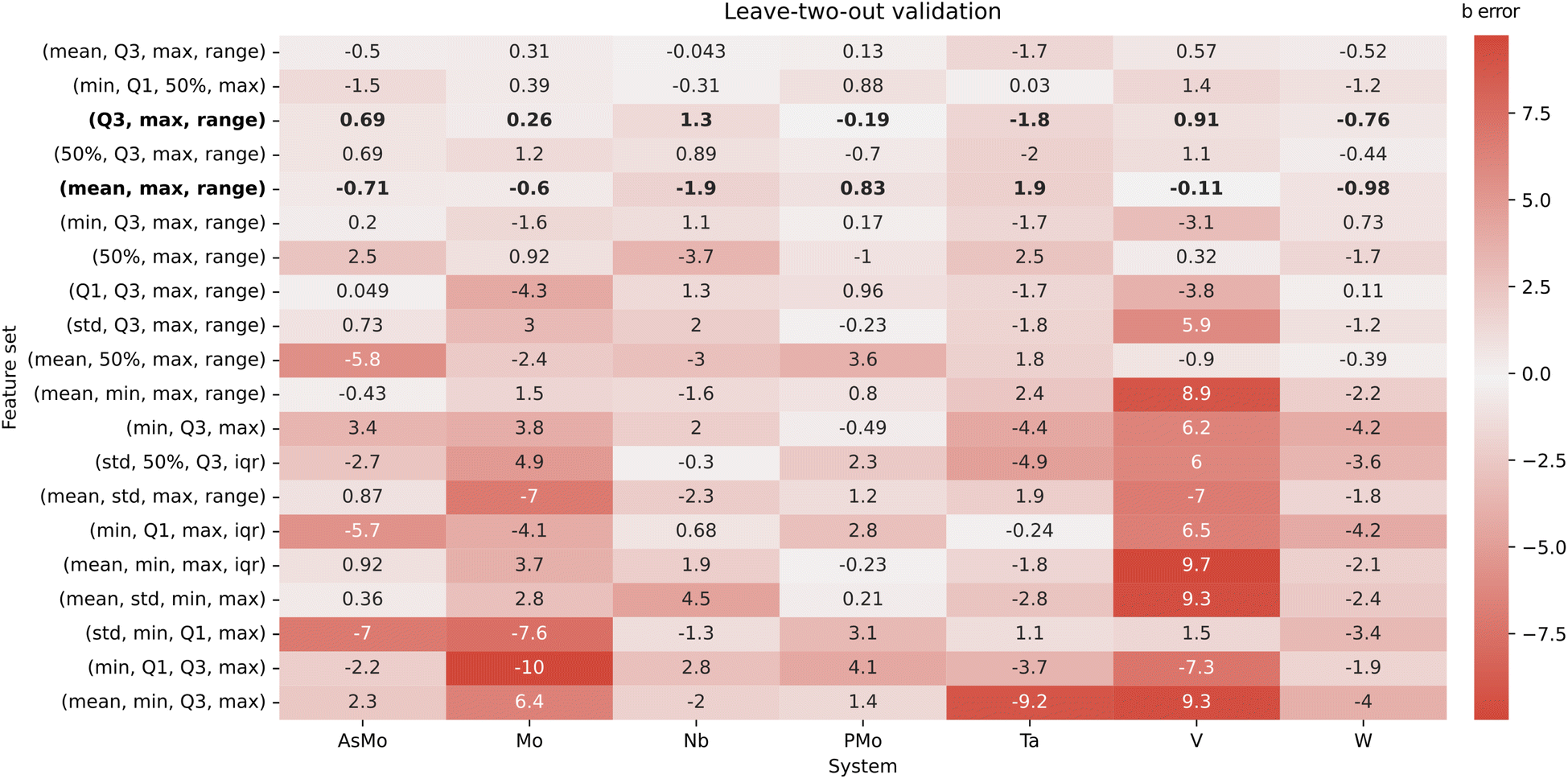Fig. 6 Heatmap representation of the leave-two-out validation. The Y-axis corresponds to the feature sets, and X-axis to the POM systems included in the study. The color scale and numeric values correspond to the difference between the median b value for every instance where a system is part of the test set and the actual values from individual regressions.

The cross-validation approach confirms the adequacy of the two aforementioned combinations of three features, which show quite low errors for all seven systems. While in principle both of them should be similarly adequate, for consistency we selected (Q₃, max, range) for further application, due to having slightly better r² and cross-validation RMSE parameters. An interesting observation arising from the cross-validation strategy is the identification of the train/test set combinations leading to larger errors. While in general the dispersion of the predicted intercepts is not too large, the situation where the test set contains both PMo and AsMo leads to important mispredictions in both intercepts (Fig. S5–S7†). This, indeed, showcases how the data-driven strategy is including a certain degree of chemical knowledge about our target systems: if no HPAs appear on the training set, the regression model cannot properly predict their intercepts. However, adding a single representative system to the training (e.g., PMo) already steers the multi-linear regression to reasonable predictions. In this way, we expect that extensions of POMSimulator to more complex systems (e.g., trimetallic structures such as PMoW) would require inexpensive re-fits of the multi-linear regression model with at least one set of experimental constants for the new system type.

As a result, we can propose an expression for the prediction of the intercept from the model trained with the six initial metal systems (without AsMo): eqn (3). In order to scale the formation constants of any given POM-based system, we can then consider the slope resulting from the general scaling in Fig. 2, m = 0.29, and then determine the intercept through eqn 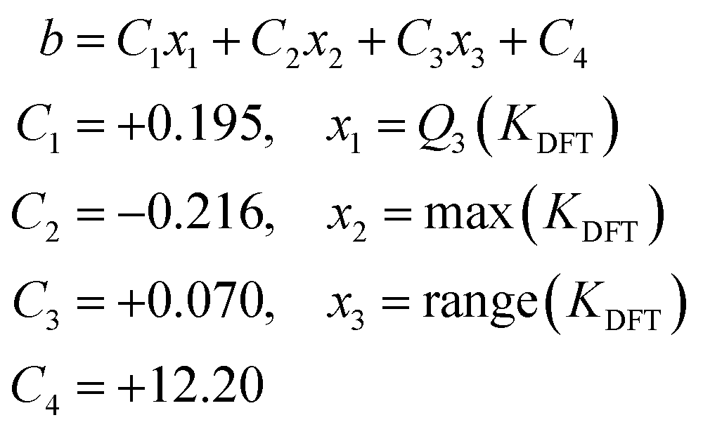(3).

In our case study on arsenomolybdates, this leads to a scaling expression in the form of

K_scaled = 0.29K_DFT − 7.29 (4)

Eqn (4) can be used to characterize the speciation across the ≈1.5 × 10⁶ models, for which we had determined formation constants. After applying the K-Means-based clusterization strategy that we previously reported for PMo, we obtained the following speciation diagrams for the 1 : 9 and 1 : 1 ratios (As : Mo) studied by Pettersson.

The speciation diagrams collected in Fig. 7 also depict the uncertainty error of our prediction, in line with our latest improvement reported for phosphomolybdates.³⁵ In general, our predictions are in very good agreement with the experimental diagrams reported by Pettersson (r² = 0.9621, Fig. 4). For the 1 : 9 ratio, {AsMo₉} species (orange and brown lines) are clearly dominant at acidic pH, with the fraction of the monomer growing quickly later on. We identify a remarkable coexistence between [AsMo₉O₃₁]³⁻ and [AsMo₉O₃₄]⁹⁻ clusters, associated with hydration/dehydration processes, reaching an approximate 50/50% split around pH = 2. Smaller peaks for the diarsenates {As₂Mo₅} (turquoise) and {As₂Mo₆} (purple) are also observed in the pH range = 4–5. Moreover, we report the formation of the previously unidentified {AsMo₆} cluster (in dark grey), right between the diarsenates and the {AsMo₉} species. The 1 : 1 ratio, corresponding to concentrations of 0.04 M for both monomers, showcases a clear dominance of the characteristic {As₂Mo₆} anion in the pH range = 0–4, which transforms into the Strandberg anion {As₂Mo₅} in the 4–6 region. From there on, only monomers are observed. We can also identify quite clearly the deprotonation processes of both clusters as pH becomes more alkaline: 2H to 1H for {As₂Mo₆} and 1H to 0H for {As₂Mo₅}. Additionally, we also report the corresponding speciation phase diagrams in Fig. S8,† completing the analysis of our target system and further proving the power of the universal scaling.

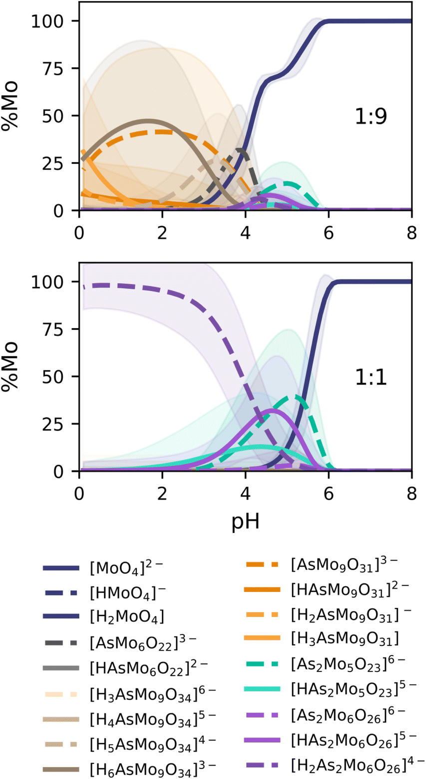Fig. 7 Speciation diagrams predicted for AsMo self-assembly reaction networks in 1 : 9 (top) and 1 : 1 (bottom) As : Mo ratios. Shading indicates the uncertainties in the concentration of the corresponding species.

Overall, the results in Fig. 7 confirm the adequacy of the proposed universal scaling scheme, combining the constant slope (m = 0.29) and the system-dependent, MLR-predicted intercept value (b = −7.29). This paves the way for the further application of POMSimulator to different polyoxometalate systems which were not accessible until now due to the lack of accurate experimental formation constants. Nonetheless, it is worth noting that the construction of the molecular set still requires some caution and chemical knowledge. Designing and calculating which building blocks should be included in the simulation is still beyond the scope of POMSimulator. The user should gather experimental evidence of important species (such as {As₂Mo₆} in the current example) and/or apply automated reaction exploration strategies, such as AutoMeKin⁴⁹ or Chemoton,⁵⁰ to ensure that all necessary building blocks and products are taken into account.

3 Conclusions

In this work we addressed one key limitation of POMSimulator's workflow related to the dependence on linearly scaling the DFT formation constants with experimental data. To determine whether a constant scaling could be found, we have analyzed the behavior of the two linear scaling parameters (slope and intercept) for six polyoxometalate systems and three DFT functionals. Our study indicates that the slope is consistently close to m = 0.3, as observed in all our previous publications. Therefore, we can conclude that DFT formation constants are overestimated by the same factor, regardless of the specific POM system and DFT functional. In contrast, the intercept has a greater variability than the slope, and when the median value was employed, the resulting speciation diagrams were chemically inaccurate. We attribute this behavior to the fact that the intercept units are also in logarithmic units, thus causing large deviation errors in the speciation results. Considering that the intercept value is not constant for all the POM systems, we have developed a multi-linear regression protocol to predict system-characteristic intercepts only using computed formation constants as input. Coupling this regression protocol with our recently developed statistical treatment of speciation diagrams, we have been able to predict the speciation of arsenomolybdates at different As : Mo ratios with a very good agreement with available experimental results.

In conclusion, the proposed universal scaling protocol supposes a decisive improvement of POMSimulator's applicability, removing the strong dependence on experimental formation constants. Thus, our methodology can be extended to POM systems where no prior experimental data are available. Moreover, we report a statistical scheme to treat other properties requiring scaling strategies, such as the characterization of accurate pK_a values.

4 Computational details

The molecular geometries of all oxo-clusters were fully optimized employing the ADF software package (SCM ADF version 2019.1),⁴⁶ using the PBE functional,^51,52 with the relativistic corrections related to the scalar-relativistic zero-order regular approximation (ZORA),^53,54 using a TZP basis set level. Solvation effects were introduced by means of the continuous solvent model COSMO with Klamt radii for water.²⁵ Stationary points were characterized with analytic frequency calculations. All Gibbs free energies were computed at 298.15 K and 1 atm, using the ideal gas-rigid rotor-harmonic oscillator (IGRRHO) model. Single point energy calculations using the BP86,^51,52,55 B3LYP^56,57 and M06L⁵⁸ functionals were also computed from the PBE optimized geometries. PBE thermochemical parameters were also employed to compute Gibbs free energies.

Data availability

A dataset collection including all DFT calculations is available in the ioChem-BD repository⁵⁹ via the following link: http://dx.doi.org/10.19061/iochem-bd-1-346. Additionally, all PBE formation constants computed with this data and used throughout this work have been included in a GitLab repository https://gitlab.com/dgarayr/pomsimulator_universal_scaling, together with the code employed to develop and validate the multi-linear regression model.

Author contributions

All authors contributed to the conceptualization of the project, which originated from an initial idea by CB and EP. DGR designed the statistical procedures and validation used in this work. JB carried out the DFT calculations. JB and DGR performed curation and formal analysis of the data, under the supervision of MSC, EP and CB, who were also responsible for funding acquisition. DGR and JB created the original draft, which was subsequently edited and reviewed by all authors.

Conflicts of interest

There are no conflicts to declare.

Acknowledgements

We acknowledge the Spanish Ministry of Science, Innovation and Universities MCIU/AEI/10.13039/501100011033 (PID2023-153344NB-I00 and CEX2019-000925-S), the European Union NextGeneration EU/PRTR (TED2021-132850B-I00), the ICIQ Foundation and the CERCA program of the Generalitat de Catalunya for funding.

Notes and references

1. IUPAC Gold Book: Chemical Speciation, 2023, https://goldbook.iupac.org/terms/view/C01023, Accessed: 2024-08-31.
2. C. Berthollet, Essai de Statique Chimique (Éd.1803), Hachette Livre, 2012.
3. A. M. M. Leal, D. A. Kulik, W. R. Smith and M. O. Saar, Pure Appl. Chem., 2017, 89, 597–643.
4. J. W. Stock, D. Kitzmann and A. B. C. Patzer, Mon. Not. R. Astron. Soc., 2022, 517, 4070–4080.
5. M. P. Humphreys, E. R. Lewis, J. D. Sharp and D. Pierrot, Geosci. Model Dev., 2022, 15, 15–43.
6. S. Haghighi, K. Askari, S. Hamidi and M. M. Rahimi, J. Open Source Softw., 2018, 3, 676.
7. A. M. Leal, Reaktoro: a unified framework for modeling chemically reactive systems, 2015, http://www.reaktoro.org/.
8. P. M. King, C. A. Reynolds and W. Richards, J. Mol. Struct.:THEOCHEM, 1990, 208, 205–221.
9. M. Schmidt am Busch and E.-W. Knapp, ChemPhysChem, 2004, 5, 1513–1522.
10. P. G. Seybold and G. C. Shields, Wiley Interdiscip. Rev.:Comput. Mol. Sci., 2015, 5, 290–297.
11. E. Wicke, M. Eigen and T. Ackermann, Z. Phys. Chem., 1954, 1, 340–364.
12. G. Zundel and H. Metzger, Z. Phys. Chem., 1968, 58, 225–245.
13. O. F. Mohammed, D. Pines, J. Dreyer, E. Pines and E. T. J. Nibbering, Science, 2005, 310, 83–86.
14. P. B. Calio, C. Li and G. A. Voth, J. Am. Chem. Soc., 2021, 143, 18672–18683.
15. Y. Tian, J. Hong, D. Cao, S. You, Y. Song, B. Cheng, Z. Wang, D. Guan, X. Liu, Z. Zhao, X.-Z. Li, L.-M. Xu, J. Guo, J. Chen, E.-G. Wang and Y. Jiang, Science, 2022, 377, 315–319.
16. M. D. Liptak and G. C. Shields, J. Am. Chem. Soc., 2001, 123, 7314–7319.
17. E. Selwa, I. M. Kenney, O. Beckstein and B. I. Iorga, J. Comput. Aided Mol. Des., 2018, 32, 1203–1216.
18. B. A. Caine, M. Bronzato, T. Fraser, N. Kidley, C. Dardonville and P. L. A. Popelier, Commun. Chem., 2020, 3, 21.
19. J. Zheng, E. Al Ibrahim and W. H. Green, ChemRxiv, 2024, preprint,  DOI:10.26434/chemrxiv-2024-vx797-v2.
20. P. G. Seybold, Mol. Phys., 2015, 113, 232–236.
21. S. Miertuš, E. Scrocco and J. Tomasi, Chem. Phys., 1981, 55, 117–129.
22. S. Miertus and J. Tomasi, Chem. Phys., 1982, 65, 239–245.
23. J. L. Pascual-Ahuir, E. Silla and I. Tuñon, J. Comput. Chem., 1994, 15, 1127–1138.
24. A. V. Marenich, C. J. Cramer and D. G. Truhlar, J. Phys. Chem. B, 2009, 113, 6378–6396.
25. A. Klamt, J. Phys. Chem., 1995, 99, 2224–2235.
26. J. Zhang, H. Zhang, T. Wu, Q. Wang and D. Van Der Spoel, J. Theor. Chem. Comput., 2017, 13, 1034–1043.
27. G. Norjmaa, G. Ujaque and A. Lledós, Top. Catal., 2022, 65, 118–140.
28. N. I. Gumerova and A. Rompel, Chem. Soc. Rev., 2020, 49, 7568–7601.
29. N. I. Gumerova and A. Rompel, Sci. Adv., 2023, 9, eadi0814.
30. K. Azmani, M. Besora, J. Soriano-López, M. Landolsi, A.-L. Teillout, P. de Oliveira, I.-M. Mbomekallé, J. M. Poblet and J.-R. Galán-Mascarós, Chem. Sci., 2021, 12, 8755–8766.
31. M. Han, W. Sun, W. Hu, Y. Liu, J. Chen, C. Zhang and J. Li, Energy Storage Mater., 2024, 71, 103576.
32. E. Petrus, M. Segado and C. Bo, Chem. Sci., 2020, 11, 8448–8456.
33. E. Petrus and C. Bo, J. Phys. Chem. A, 2021, 125, 5212–5219.
34. E. Petrus, M. Segado-Centellas and C. Bo, Inorg. Chem., 2022, 61, 13708–13718.
35. J. Buils, D. Garay-Ruiz, M. Segado-Centellas, E. Petrus and C. Bo, Chem. Sci., 2024, 15, 14218–14227.
36. E. Petrus, J. Buils, D. Garay-Ruiz, M. Segado-Centellas and C. Bo, petrusen/pomsimulator: Release 1.0.0, 2024,  DOI:10.5281/zenodo.10689769.
37. E. Petrus, J. Buils, D. Garay-Ruiz, M. Segado-Centellas and C. Bo, J. Comput. Chem., 2024, 45, 2242–2250.
38. E. Petrus, D. Garay-Ruiz, M. Reiher and C. Bo, J. Am. Chem. Soc., 2023, 145, 18920–18930.
39. P. Pracht, R. Wilcken, A. Udvarhelyi, S. Rodde and S. Grimme, J. Comput. Aided Mol. Des., 2018, 32, 1139–1149.
40. J. Cruywagen, Advances in Inorganic Chemistry, Elsevier, 1999, vol. 49, pp. 127–182.
41. G. M. Rozantsev and O. I. Sazonova, Russ. J. Coord. Chem., 2005, 31, 552–558.
42. K. Elvingson, A. González Baró and L. Pettersson, Inorg. Chem., 1996, 35, 3388–3393.
43. N. Etxebarria, L. A. Fernández and J. M. Madariaga, J. Chem. Soc., Dalton Trans., 1994, 3055–3059.
44. G. J.-P. Deblonde, A. Moncomble, G. Cote, S. Bélair and A. Chagnes, RSC Adv., 2015, 5, 7619–7627.
45. L. Pettersson, I. Andersson and L. O. Oehman, Inorg. Chem., 1986, 25, 4726–4733.
46. G. te Velde, F. M. Bickelhaupt, E. J. Baerends, C. Fonseca Guerra, S. J. van Gisbergen, J. G. Snijders and T. Ziegler, J. Comput. Chem., 2001, 22, 931–967.
47. E. Baerends, D. Ellis and P. Ros, Chem. Phys., 1973, 2, 41–51.
48. L. Pettersson, B. Carlsson, S. Rundqvist, A. F. Andresen and P. Fischer, Acta Chem. Scand., 1975, 29a, 677–689.
49. E. Martínez-Núñez, G. L. Barnes, D. R. Glowacki, S. Kopec, D. Peláez, A. Rodríguez, R. Rodríguez-Fernández, R. J. Shannon, J. J. P. Stewart, P. G. Tahoces and S. A. Vazquez, J. Comput. Chem., 2021, 42, 2036–2048.
50. J. P. Unsleber, S. A. Grimmel and M. Reiher, J. Chem. Theory Comput., 2022, 18, 5393–5409.
51. J. P. Perdew, Phys. Rev. B:Condens. Matter Mater. Phys., 1986, 33, 8822–8824.
52. J. P. Perdew, Phys. Rev. B:Condens. Matter Mater. Phys., 1986, 34, 7406.
53. E. Van Lenthe, E. J. Baerends and J. G. Snijders, J. Chem. Phys., 1993, 99, 4597–4610.
54. E. Van Lenthe and E. J. Baerends, J. Comput. Chem., 2003, 24, 1142–1156.
55. A. D. Becke, Phys. Rev. A, 1988, 38, 3098–3100.
56. C. Lee, W. Yang and R. G. Parr, Phys. Rev. B:Condens. Matter Mater. Phys., 1988, 37, 785–789.
57. A. D. Becke, J. Chem. Phys., 1993, 98, 5648–5652.
58. Y. Zhao and D. G. Truhlar, J. Chem. Phys., 2006, 125, 194101.
59. M. Álvarez-Moreno, C. De Graaf, N. López, F. Maseras, J. M. Poblet and C. Bo, J. Chem. Inf. Model., 2015, 55, 95–103.

---

Footnotes

† Electronic supplementary information (ESI) available. See DOI: https://doi.org/10.1039/d4dd00358f

‡ These authors contributed equally to this work.

---