Opentrons for automated and high-throughput viscometry

Abstract

We present an improved high-throughput proxy viscometer based on the Opentrons (OT-2) automated liquid handler. The working principle of the viscometer lies in the differing rates at which air-displacement pipettes dispense liquids of different viscosities. The operating protocol involves measuring the amount of liquid dispensed over a set time for given dispense conditions. Data collected at different set dispense flow rates was used to train an ensemble machine learning regressor to predict Newtonian liquid viscosity in the range of 20–20 000 cP, with ∼450 cP error (∼8% relative to sample mean). A phenomenological model predicting the observed trends is presented and used to extend the applicability of the proxy viscometer to simple non-Newtonian liquids. As proof-of-concept, we demonstrate the ability of the proxy viscometer to characterize the rheological behavior of two types of power-law fluids.

---

Introduction

With the advent of lab automation and artificial intelligence (AI), there has been a drive to accelerate materials discovery and development by moving towards closed-loop, autonomous experimentation.^1,2 Lab automation streamlines the experimentation process, while machine learning algorithms assist in analyzing data and suggesting the next set of experiments based on performance predictions. The successful coupling of robotic experiments and AI enables data collection and decision making to occur without human intervention. This approach can be used to explore large experimental design spaces in a time- and resource-efficient manner.

Viscosity is a key physical property of many products, hence the measurement of viscosity plays a critical role in a wide range of industries, from pharmaceuticals^3,4 to cosmetics^5,6 and food production.⁷ The traditional methods of measuring viscosity are typically time-consuming and labor-intensive. For example, a single run on a rotational rheometer requires careful sample loading and instrument calibration, followed by thorough cleaning after the measurement. High-throughput is becoming a priority for rapid screening purposes, particularly with many industries looking to re-formulate their portfolio of products to meet sustainability and regulatory pressures.^8–11 Alternate methods for measuring viscosity have been developed, such as microfluidic-based rheometers.^12–14 However, such techniques cannot attain the degree of throughput and automation required for screening large numbers of samples. Automated rheometers are available commercially, but these are expensive and difficult to integrate into larger workflows. There remains a need for an easily accessible solution to automated, high-throughput viscometry.

In this paper, we extend prior work¹⁵ on an automated and high-throughput method of measuring viscosity based on the Opentrons (OT-2) pipetting robot. The key extensions are an increase in applicable viscosity range for Newtonian liquids through implementation of real-time mass measurements and the integration of an analytical model to extend the proxy viscometer to non-Newtonian liquids. These improve the versatility of the platform, for example by enabling the screening of low-viscosity fluids, and represent a significant stride towards a more general-use proxy viscometer. The working principle of the proxy viscometer leverages the differing ability of air-displacement pipettes in dispensing liquids with varying viscosities. Under given dispense conditions, the actual amount of liquid dispensed depends on the liquid viscosity. We measure the amount of liquid dispensed over time for a range of dispense flow rates and liquid viscosities (for Newtonian fluids) and train a regression model to predict liquid viscosity within the range of 20 to 20 000 cP. We develop an analytical model to describe the experimental results and extend the model to a simple non-Newtonian (power-law) liquid, demonstrating proof-of-concept cases on molasses and a surface cleaner. A single viscosity measurement on our proxy viscometer takes ∼1.5 minutes and requires minimal human intervention. Moreover, the Opentrons is cost-effective, readily integrated into workflows and uses open-source software, all of which have resulted in its widespread use in automated workflows.^16–18

Methods and materials

Proxy viscometer setup

The operating platform of the proxy viscometer is the Opentrons (OT-2), an affordable and open-source automated pipetting robot (Fig. 1). One of the deck slots on the OT-2 was removed to allow a precision balance (Mettler Toledo MS303TS/00) to be incorporated in the setup.¹⁹ The pipette tips used for measurements are 1000 μL wide bore tips (Fisher Scientific). A technical drawing of the tips is provided in the ESI.† The working principle of the proxy viscometer has been described in detail previously.¹⁵ Briefly, air-displacement pipettes operate by maintaining an air cushion between the plunger and fluid. The cushion volume is sensitive to the fluid's physical properties, especially viscosity, and therefore, liquids of different viscosities will be dispensed differently under the same dispense conditions. This difference in measured dispense behavior serves as a proxy for viscosity.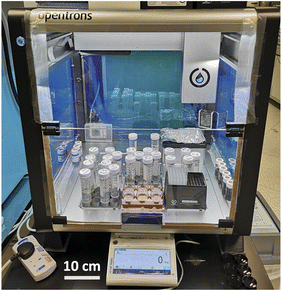

Fig. 1 Experimental setup for the high-throughput viscometer: automated liquid handling robot Opentrons (OT-2) with a precision balance fitted beneath the dispense plate.

Proxy viscometer operation

The protocol for a single measurement involves two stages: aspiration and dispense (Table 1). During the aspiration stage, the pipette tip is lowered into the liquid reservoir and liquid is aspirated at a set aspiration flow rate, here 100 μL s⁻¹. The amount of liquid aspirated is calculated based on the expected amount of liquid to be dispensed over 10 s. For example, a total of 100 μL is aspirated for a set dispense flow rate of 10 μL s⁻¹, while a total of 800 μL is aspirated for a set dispense flow rate of 80 μL s⁻¹. A delay of 30 s is included to allow for the air pocket between the plunger and the liquid to reach equilibrium, a step that enables accurate aspiration of viscous liquids. After the pipette is charged, the pipette tip is touched to the four sides of the reservoir to remove trailing liquid on the outside of the tip (touch tip). This step is repeated at three different heights to remove liquid at different positions along the tip exterior. The pipette tip is then moved to the dispense plate for the start of the dispense stage.

Table 1 Operating protocol for a single measurement of fluid viscosity using the Opentrons

Stage	Step	Description
Aspiration	Pick up pipette tip	Begin a run
	Aspirate fluid at 100 μL s^−1	Withdraw fluid from reservoir
	Delay for 30 s	Allow for equilibration of air pressure
	Touch pipette tip to four sides of the well, performed at three different heights	Remove droplets on various locations of pipette tip exterior
	Move pipette tip to dispense plate	Aspiration stage complete
Dispense	Dispense fluid at set flow rate for 10 s	Weigh fluid dispensed from pipette tip
	Delay for 30 s	Allow remaining fluid to drip
	Dispose pipette tip	Dispense stage complete

---

For a given set dispense flow rate, the liquid is dispensed for 10 s and the amount of liquid collected on the plate is measured at intervals of 0.2 s. After 10 s, there is a delay of 30 s to allow any remaining droplets to fall onto the dispense plate. The pipette tip is then disposed of and a single measurement is concluded within 1.5 minutes. Five replicates were carried out for each fluid tested. The pipette tip was changed between each replicate. The key difference in measurement protocols between this work and previous work lies in the measurement of the mass of fluid. Previously, the mass of fluid dispensed was measured at a single time point, at the end of the dispensing step;¹⁵ in this work, the mass of fluid dispensed is measured in real time, providing higher-fidelity information about the dispensing process and thus enabling us to extend the viscosity range of the proxy viscometer.

Liquids

The Newtonian liquids tested consisted of a range of general purpose mineral oil viscosity standards (Paragon Scientific) and their mixtures under ambient lab temperature conditions. The viscosities of mixtures of standards were determined by a rotational rheometer using parallel plates (TA Instruments DHR-3). The densities of mixtures were measured by aspirating a known volume of liquid with a positive displacement pipette and dispensing onto a precision balance. A total of 40 Newtonian liquids were tested. The Newtonian standards used in the experiments are listed in Table S1 in ESI.†

Two non-Newtonian liquids tested for proof-of-concept purposes were molasses (Brer Rabbit) and Cif cream surface cleaner (Unilever). Cif is a non-colloidal suspension of non-spherical calcium carbonate particles (average size around 50 μm) in a viscous binder. The rheological behavior of each fluid was measured at 25 °C using steady state shear rate sweeps on a rotational rheometer with parallel plates. Three replicates were performed for each fluid and the average values are reported. The densities were measured as described for the Newtonian standards.

Results and discussion

Dynamic fluid dispense curves

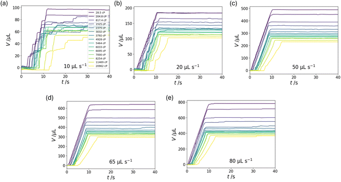
Fig. 2 shows the measured volume of liquid dispensed, V, as a function of time, t, for ten selected Newtonian standards at five different set dispense flow rates, where t = 0 corresponds to the start of the dispense stage. Generally, liquids with lower viscosities are dispensed at a faster rate compared to liquids with higher viscosities. For the slowest dispense flow rate, of 10 μL s⁻¹, the liquid tends to be dispensed intermittently as discrete droplets due to the balance between surface tension and gravity, resulting in a stepped dispense profile. At higher flow rates, the liquid is dispensed as a stream, resulting in continuous collection profile after an initial delay corresponding to the formation of the initial droplet.

Fig. 2 Volume of Newtonian liquid dispensed with time during the proxy viscometer measurement protocol for select liquid viscosities and a range of set dispense flow rates: (a) 10 μL s⁻¹, (b) 20 μL s⁻¹, (c) 50 μL s⁻¹, (d) 65 μL s⁻¹ and (e) 80 μL s⁻¹.

For each dispense profile, we fit the following sigmoid function to the data:

where V_plat is the volume dispensed at long times, and m and s are positive constants with units of time. When t = m, V = V_plat/2, therefore m is a characteristic timescale associated with reaching half the final dispensed volume. In Fig. 3(a), we show dispense profiles for five replicates of the measurement protocol with a Newtonian standard (6033 cP) at a set dispense flow rate of 80 μL s⁻¹, alongside fits to eqn (1). The sigmoid function fits the data well and there is good repeatability between the five replicates. The experimental data show a sharp transition after 10 s, corresponding to the cessation of piston motion, which the sigmoid function cannot reproduce.

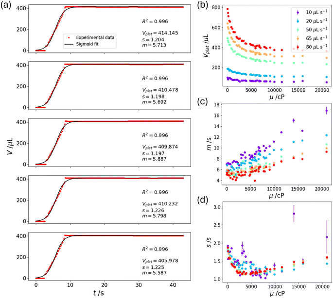Fig. 3 Sigmoid fits to the dispense curves. (a) Five replicates of the measurement protocol for a Newtonian standard with viscosity of 6033 cP at a set dispense flow rate of 80 μL s⁻¹. The black lines are fits of eqn (1) to the red experimental data points. The fit parameters to eqn (1) for all measured viscosities and set dispense flow rates are plotted: (b) V_plat, (c) m and (d) s.

The fitted parameters V_plat, m and s for the Newtonian liquids are plotted as a function of viscosity in Fig. 3(b)–(d). We observe strong relationships between the fitted parameters and viscosity, especially for V_plat, suggesting that regression models can be trained to predict liquid viscosity. Generally, with an increase in viscosity, V_plat decreases and m increases. This corresponds to smaller final dispense volume for liquids with higher viscosities and the liquids being dispensed at a slower average rate.

Regression model for Newtonian liquids

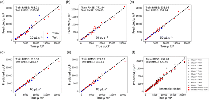
To build a tool for viscosity prediction of Newtonian liquids, we trained several models on the data for each set dispense flow rate. Specifically, we trained linear regression, support vector regression, ridge regression and Gaussian process regression models (see ESI† for more details). These models were selected for their simplicity and flexibility in modelling low-dimensional data spaces well. The input variables to the models were the fitted parameters V_plat, m and s, and the target variable was liquid viscosity. The dataset collected at each dispense flow rate was split into training and testing sets using a stratified 75–25% split. We optimized the models by tuning the hyperparameters and evaluated the root mean squared errors (RMSE) for the train and test sets, based on which we selected the best performing regression models. For every set dispense flow rate, we found support vector regression (SVR) with RBF kernel to give the smallest errors (Fig. 4). Therefore, a support vector regression model was used to train the datasets at each set dispense flow rate. The model trained on data from higher set dispense flow rates tended to give more accurate predictions, evident from the smaller train and test RMSE values. This is attributed to the more continuous dispense profiles and better fits to a sigmoid function.

Fig. 4 Support vector regression model trained on data at different set dispense flow rates: (a) 10 μL s⁻¹, (b) 20 μL s⁻¹, (c) 50 μL s⁻¹, (d) 65 μL s⁻¹ and (e) 80 μL s⁻¹. Predictions from the model trained on datasets collected at each set dispense flow rate are weighted by the train RMSE value and averaged to produce an ensemble model.

Since the viscosity of a Newtonian liquid is independent of the applied shear rate, we expect the regression model trained on different set dispense flow rates to predict similar viscosities. As such, we developed an ensemble model by taking a weighted average of the viscosity predictions from the models at different flow rates, where the weighting was based on the train RMSE values, i.e., individual model accuracies. As seen from Fig. 4(f), the weighted ensemble model outperforms the model trained on the individual flow rate datasets, with train and test RMSE values of ∼450 cP (∼8% relative to sample mean). We note that the ensemble model presents only a marginal improvement in accuracy over the model trained on the individual flow rate datasets (for dispense flow rates larger than 10 μL s⁻¹). Hence, the ensemble model can be employed if a user prioritizes accuracy over speed. Otherwise, the user can run the measurement protocol at only one set dispense flow rate (≥20 μL s⁻¹) and use the model trained on a single flow rate to obtain a less accurate prediction. This might be desirable for the rapid screening of many samples.

Analytical model

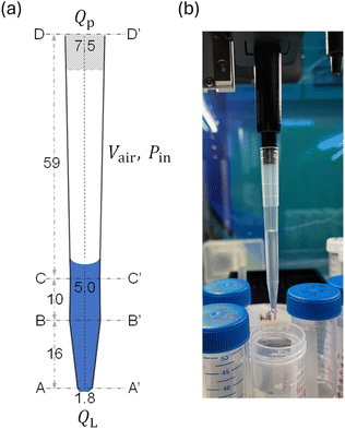
The prediction of viscosity for non-Newtonian liquids is complex because of the shear rate dependence. We can envision extending the regression model for Newtonian liquids to estimate a rheological curve for non-Newtonian liquids through a proxy steady-state shear rate sweep. For example, we can calculate the shear rates associated with different set dispense flow rates, train Newtonian models for the dispense flow rates that correspond to the shear rates of interest, then predict the viscosity at the selected flow rates. This is similar to the methodology outlined by Deshmukh et al.²⁰ However, this approach is dependent on the model trained for each dispense flow rate being accurate. For low set dispense flow rates that correspond to small shear rates, the model might not be accurate enough for a reliable viscosity prediction.

To circumvent this, we develop a phenomenological model that can be applied to non-Newtonian liquids. Consider the pipette tip in Fig. 5: the pipette operates by firstly immersing the tip below the surface of the sample liquid. The plunger motion initially expels air through the tip and then draws liquid up as the plunger withdraws and creates suction in the tip cavity. The pipette tip is then moved out of the liquid. Fig. 5(a) shows the configuration: V_air is the volume of air in the cavity at internal pressure P_in. During the dispense stage, the plunger moves downward, its motion occupying volume at a rate Q_p. The air in the cavity is compressed, increasing P_in and this causes the liquid to leave through the tip at volumetric flow rate Q_L : Q_L is determined by the geometry of the pipette tip, the rheology of the liquid and the instantaneous pressure difference P_in − P_atm, where P_atm is the pressure of the surroundings.

Fig. 5 Experimental setup (a) schematic of pipette tip and (b) photograph of Thermo Scientific 1000 μL wide bore pipette after the aspiration stage. Diameter of the duct at locations AA′, BB′/CC′ and DD′ and distances AB, BC and CD indicated, all dimensions in mm.

Assuming that the tip walls are rigid and the liquid is both involatile and incompressible, a volume balance on region ADD′A′ yields

where t is time. Treating the air as an ideal gas and assuming isothermal compression,where V₀ and P₀ are the initial air volume and internal pressure, respectively. These quantities were not measured in tests and are also expected to depend on the liquid. The values of P₀ are likely to lie below atmospheric (around 101 kPa, subject to variation), as the sum of P₀, the capillary pressure jumps across the interfaces and the hydraulic head of liquid in the pipette tip is equal to atmospheric pressure on that day. The pipette tip dimensions set an upper limit on V₀ of 5000 μL, and measurements by Deshmukh et al.²⁰ indicate P₀ of order 10 kPa (gauge).

Contributions from gravity and capillary action are neglected in the flow model. The pressure difference associated with a drop at the pipette tip is of order 2Γ/R_AA′, where Γ is the surface tension and R_AA′ is the radius of the duct at the tip exit (of order 1 mm). For water at 20 °C, this gives a pressure difference of order 150 Pa for a hemispherical drop, which would halve if the liquid leaves as a cylindrical thread. These differences are small when compared to the pressure required to expel a viscous liquid (see below), but capillary action could impose an initial lag before the first drop is collected.

Inertia and transients in flow are neglected and Q_L is modelled assuming instantaneous steady state, with the pressure drop dominated by that required to pass through the converging conical duct ABB′A′. The Cogswell result²¹ for converging flow of a power-law fluid with shear stress σ related to shear rate [small gamma, Greek, dot above] by

σ=K[small gamma, Greek, dot above]ⁿ (4)

in which K is the consistency and n the flow index, iswhere α is the half angle of the conical duct. For the wide bore pipette tip in Fig. 5, with α = 6.1°, this reduces to

The first term on the RHS is the apparent shear rate, [small gamma, Greek, dot above]_app, and the flow rates studied by Soh et al.,¹⁵ of 5–100 μL s⁻¹, in the pipette tip in Fig. 5 correspond to shear rates of 9–175 s⁻¹. Eqn (6) can be written as

P_in − P_atm = BQ_Lⁿ (7)

yielding the governing equation

Introducing m = n⁻¹ and p = P_in − P_atm, gives (with Q_p constant as in the tests)

Rearranging gives

Since p(t = 0) ∼ 0, this predicts that p (and P_in) will initially increase and approach a limit asymptotically, where p_lim = BQ_pⁿ, i.e. Q_L = Q_p: the air in the cavity undergoes compression until the pressure is sufficiently high to drive the liquid out at the rate set by the piston.

The instantaneous liquid flow rate is set by p and the volume dispensed after experiment duration t_E is

If m is integral, one could evaluate eqn (8) using Laplace Transforms. This was not attempted here and eqn (11) was evaluated numerically (see ESI†).

Newtonian liquids

For Newtonian liquids, n = 1 and eqn (9) yields an analytical result relating the flow rate ratio θ = 1 − Q_L/Q_p and dimensionless time τ = t/t_C (where t_C = V₀P₀/βμQ_P², see ESI†)Here c′ = 1 + P_atm/βμQ_p, μ is the liquid viscosity and the product βμ corresponds to B in eqn (7) for the Newtonian case. Whilst this result allows the instantaneous flow rate to be evaluated directly, V(t) requires numerical integration.

For the pipette tip in Fig. 5, β = 15 × 10⁹ Pa s m⁻³. Taking P₀ = 101 325 Pa, V₀ = 2000 μL and a set dispense rate, Q_p, of 80 μL s⁻¹, t_C is given by 2083/μ and c′ = 1 + 83.3/μ. The characteristic timescale in eqn (12) is then t_C/c′². For a 6 Pa s liquid, representative of those considered by Soh et al.,¹⁵ c′ = 14.9 and t_C is 347 s, giving a characteristic timescale of 1.6 s, which is comparable with the length of the dispense times (5–10 s): the flow rate will change noticeably over the duration of a test with a viscous liquid due to air compression. For less viscous solutions, assuming P₀ ∼ P_atm, the characteristic time scale will be approximately βμV₀/P₀: for aqueous solutions, with μ ∼ 1 mPa s, this is of order milliseconds and the pipette will dispense accurately.

For the 6 Pa s liquid, the ratio of the pressure drop across the pipette tip to that across Section BC is >40, justifying neglecting the contribution from above BB’ for this and other liquids tested by Soh et al.¹⁵ Fig. 6 presents a series of model predictions for Newtonian liquids with viscosity 6.08 Pa s at a set dispense flow rate of 80 μL s⁻¹. The numerical integration of eqn (10) matches eqn (12). The flow rate approaches Q_p after 6 s, so the volume collected after 5 s or 10 s (as used by Soh et al.¹⁵) will be noticeably less than Q_pt_E in both cases for this viscous liquid.

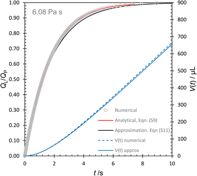Fig. 6 Predicted evolution of scaled flow rate and volume dispensed from the pipette tip in Fig. 5 for a 6.08 Pa s Newtonian liquid with Q_p = 80 μL s⁻¹, P₀ = 101325 Pa and V₀ = 2000 μL.

Soh et al.¹⁵ tested 33 Newtonian viscosity standards and reported the amount of liquid collected over time t_E as the averaged flow rate, Q̄ = V(t_E)/t_E. They found that Q̄ varied systematically with viscosity as Q̄ ∝ μ^−1/3, thereby offering a simple method of estimating the liquid viscosity. We demonstrate here that this result can be predicted by the model. For a Newtonian liquid, for large values of c′ (as in their tests), an approximate form of eqn (12) is (see ESI†)

This can be integrated analytically to obtain the volume dispensed, giving the profile in Fig. 6 which follows the exact result closely. Writing the reciprocal of the characteristic time as φ, the analytical result for Q̄ is

Fig. 7 shows eqn (14) predicts the form of the experimental results reported by Soh et al.¹⁵ and gives good agreement with the Q̄ ∝ μ^−1/3 relationship they obtained by a regression fit to their data set. Better agreement could be obtained by adjusting the model parameters P₀ and V₀ for each case, but the uncertainty regarding the effect of capillarity and flow onset would remain. Soh et al.¹⁵ presented a scaling argument explaining the Q̄ ∝ μ^−1/3 relationship which did not consider the role of air compression in the flow mechanism. This model corrects that oversight and demonstrates the importance of air compression by analyzing V(t) data series collected in related experiments.

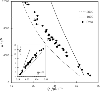Fig. 7 Comparison of predicted effect of viscosity on average flow rate for Newtonian viscosity standards reported by Soh et al. (2023) for tests with dispense period of 5 s and Q_p = 50 μL s⁻¹. Error bars indicated 95% confidence interval from 9 repeats. Loci show predictions of simplified model, eqn (14), with parameters P₀ = 101325 Pa, V₀ values indicated. Inset shows the data in the linearized form reported by Soh et al.

Soh et al.¹⁵ also demonstrated that the pipette tip design affected the volume of liquid collected (and hence Q̄). Their data, reproduced in Fig. 8, showed that a standard pipette tip (see ESI†), with smaller exit orifice, was more sensitive to liquid viscosity than the wide-bore tip in Fig. 5. A custom pipette geometry gave an intermediate response which was almost linearly sensitive to viscosity. Fig. 8 shows that these behaviors can be predicted by eqn (14). A single set of model parameters was used in the simulations in this case; better agreement could be obtained by matching these to the individual pipette tips as they have different filling characteristics.

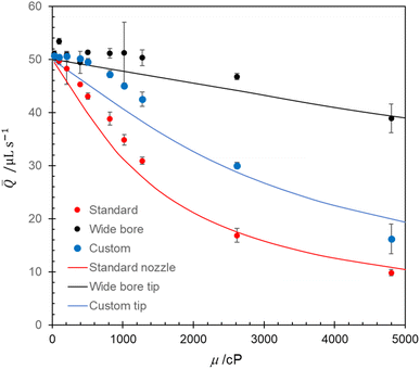Fig. 8 Effect of Newtonian viscosity on predicted average flow rate (eqn (14)) for different tip designs, Q_p = 50 μL s⁻¹, 5 s dispense period. Points – experimental data, error bars indicated 95% confidence interval from 9 repeats. Loci – model predictions, with P₀ = 101325 Pa and V₀ = 2000 μL for both nozzles. β values – standard, 13.6 × 10¹⁰ m⁻³; custom, 6.2 × 10¹⁰ m⁻³; wide bore 1.5 × 10¹⁰ m⁻³.

Newtonian liquids: comparison with experimental results

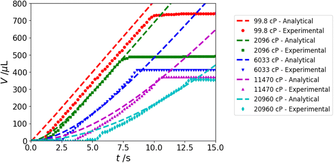
To demonstrate the robustness of the model, we can compare the analytical solution, as presented in eqn (12), to experimental results. Setting V₀ = 8000 μL and P₀ = 95 kPa, we solve the analytical model for Newtonian fluids with a range of viscosities. Fig. 9 shows the solution to the analytical model for a set dispense flow rate of 80 μL s⁻¹ alongside experimental dispense curves, from which we observe good agreement. While the trained support vector regression model gives reasonable predictions of liquid viscosity for Newtonian fluids, having an accurate analytical model paves the way for extending the proxy viscometer to non-Newtonian liquids. In selecting the values of V₀ and P₀, we first set P₀ based on the range of values reported by Deshmukh et al.,²⁰ then determined the value of V₀ that resulted in the best fits. We recognize that the value obtained is greater than the limit set by the pipette geometry, and note that the choice of V₀ also depends on P₀, which was not measured in these experiments.

Fig. 9 Comparison between analytical model and experimental data for Newtonian fluids with different viscosities at a set dispense flow rate of 80 μL s⁻¹. Points – experimental data. Dotted lines – model predictions, with P₀ = 95 kPa and V₀ = 8000 μL.

Power-law fluids

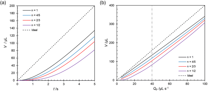
The scope for studying non-Newtonian liquids using the pipetting system is investigated conceptually here for the simplest case of a time-independent (Generalized Newtonian) fluid, the power-law fluid, eqn (4). The numerical model, eqn (10) was used to predict the instantaneous flow rate and volume discharged for shear-thinning fluids with n in the range 0.5–1.0. To facilitate comparisons, the value of the consistency factor K was adjusted to give an apparent viscosity of 6 Pa s at a shear rate of 99 s⁻¹ corresponding to the exit conditions when Q_p = 40 μL s⁻¹). Fig. 10(a) shows that compression of the air pocket has a significant effect at this flow rate for these viscous liquids. The effect is stronger for shear-thinning fluids as the initial increase in pressure induces a low flow rate (and apparent shear rate), giving rise to a high apparent viscosity. At the end of the dispense period, the volume collected increases with n. Fig. 10(b) shows that the difference between the fluids decreases at higher dispense rates, as the apparent viscosity of the fluids is decreased by the higher flow rates. The difference in measured volumes has already been shown to reflect a difference in viscosity for Newtonian liquids, and that difference will depend on t_E (eqn (14)).

Fig. 10 Predicted volume dispensed during a 5 s dispense period for power-law fluids with 0.5 ≤ n ≤ 1 in the wide bore tip. Model parameters P₀ = 101 325 Pa and V₀ = 2000 μL. The power-law consistency was adjusted such that each liquid had the same apparent viscosity, or 6 Pa s, at the apparent shear rate in the pipette tip at Q_p = 40 μL s⁻¹ (indicated by vertical dot-dashed line), of 99 s⁻¹. (a) Dispense profile for Q_p = 40 μL s⁻¹, dashed line shows ideal case, V = Q_pt; (b) effect of set dispense rate.

Power-law fluids: comparison with experimental results

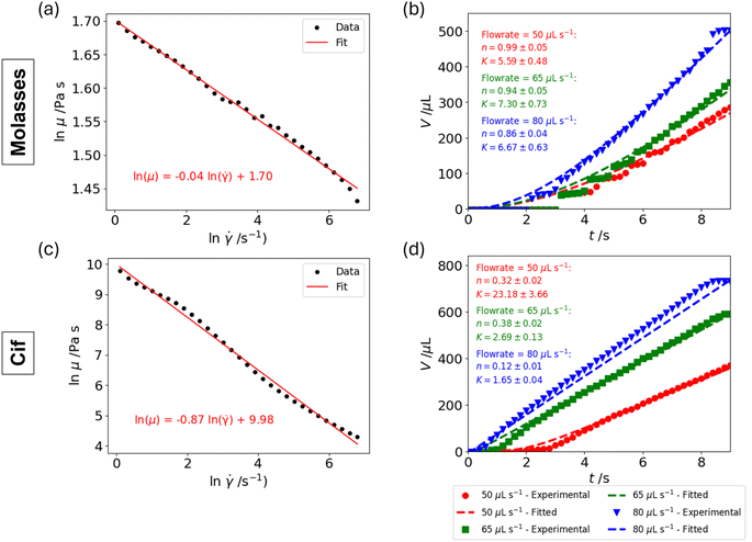
The power of the analytical model is that it enables us to extract the non-Newtonian fluid parameters, n and K, from the liquid dispense curves. The range of dispense flow rates used in the experimental setup generates apparent shear rates at the pipette tip exit between 18 s⁻¹ and 140 s⁻¹ (see first term on RHS of eqn (6)); the ability to study a non-Newtonian fluid is dependent on whether the fluid viscosity changes noticeably over this range of shear rates. Given that the tests involve two quantities (volume and time) over one decade of shear rate, a constitutive model with only two degrees of freedom is appropriate. As proof-of-concept, we demonstrate the approach on molasses and a surface cleaner (Cif), both shear-thinning liquids that can be described as power-law fluids.²² The rheological behaviors of molasses and Cif were characterized using a rotational rheometer and the viscosity-shear rate curves were fitted to a power-law relation to obtain K and n (Fig. 11(a) and (c)). Specifically, we fitted the logarithm of viscosity versus logarithm of shear rate to a linear equation of form ln (μ) = a ln ([small gamma, Greek, dot above]) + b, where n = a + 1 and K = exp(b).

Fig. 11 Fitting of analytical model to experimental data for power-law fluids to estimate rheological parameters. (a) and (c) Plot of viscosity as a function of shear rate of molasses (a) and Cif cream surface cleaner (c), as measured by a rheometer. The red lines are linear fits to the black experimental points, from which the power-law fluid parameters n = 0.96 and K = 5.48 Pa s for molasses and n = 0.13 and K = 20.69 Pa s for Cif can be calculated. (b) and (d) Fits of the analytical model to experimental data for molasses (b) and Cif (d) at different set dispense flow rates. Points – experimental data. Dotted lines – fitted model with P₀ = 95 kPa, and V₀ = 8000 μL. The extracted parameters n and K from each fit and associated 95% confidence intervals (estimated from sensitivity analysis) are annotated.

The dispense profiles were obtained by running the measurement protocol on power-law fluids at different set dispense flow rates. We used differential evolution to minimize the mean squared error between the numerical model and experimental data, with ln(K) and n as the fitted parameters. Due to the disparity in scales of K and n, we optimized over ln(K) instead of K to ensure better convergence. Furthermore, we applied L2 regularization terms to K and n, which penalize excessively large parameter values and help to balance the optimization between the fitted parameters. We imposed the following bounds for the fit: 0.001 Pa sⁿ ≤ K ≤ 10 Pa sⁿ and 0.1 ≤ n ≤ 1 for molasses; 1 Pa sⁿ ≤ K ≤ 30 Pa sⁿ and 0.1 ≤ n ≤ 1 for Cif. We note that the regularization terms and bounds should be adjusted for optimal fits depending on the fluids of interest. For the model, we selected values of P₀ = 95 kPa and V₀ = 8000 μL. Sensitivity analysis was conducted to calculate the 95% confidence intervals using a perturbation method, i.e. by systematically perturbing the best-fit parameters in small increments and recalculating the loss function until it exceeded a given threshold value.

Fig. 11(b) and (d) show the experimental dispense profiles and fitted solutions for several set dispense flow rates, displaying good fits to the data. We consider only the dispense profiles at high set dispense flow rates (≥50 μL s⁻¹) because the stepped profiles at low flow rates result in unreliable fits. Despite the underlying assumptions of the analytical model, the extracted values of K and n are usefully close to the actual values. For molasses, the errors for the fitted K values are between 2% and 33% and for the fitted n values are between 2% and 10% across the three set flow rates; for Cif, the errors for the fitted K values are between 7% and 92% and for the fitted n values are between 8% and 192% across the three set flow rates. We acknowledge that the errors arising from the fits can be large and there is room for improvement through refinement of the model. Nevertheless, considering the wide, general bounds for K and n implemented for the fits, these results show promise in the proxy viscometer being used to screen rheological behavior in simple non-Newtonian liquids.

The following workflow would be used to characterize a fluid anticipated to exhibit power-law behavior:

(1) Run the experimental protocol at a high, low and intermediate flow rate.

(2) Compare the apparent viscosity obtained for the three flow rates. If these differ within the bounds of measurement uncertainty, and show a systematic change with increasing flow rate, run the protocol for further flow rates to collect a larger data set (in this work, five were used).

(3) Select bounds for n and K. Prior approximation of the fluid flow behavior would be useful, for example, shear-thinning or shear-thickening, and expected broad range for the consistency coefficient.

(4) Select regularization terms for n and K. The terms can be tuned algorithmically for best agreement across fits from the different flow rate data and to avoid being stuck at the imposed bounds.

(5) Perform the fits and average extracted parameters across different flow rate data.

It should be noted that many non-Newtonian fluids exhibit constant viscosity at low shear rates, and the ability to capture this behavior depends on the ability to access a wide window of shear rates.

Discussion

The proxy viscometer outlined in this work enables fast and automated measurement of liquid viscosity (1.5 minutes per run). Depending on purpose, the user can decide on the number of set dispense flow rates to run per sample. If speed in testing is priority, the user can run the measurement protocol at a high set dispense flow rate and use the prediction from the model trained on an individual flow rate dataset; if accuracy is prioritized over speed, the user can run the protocol at all set dispense flow rates and use the weighted ensemble model. While more time is required to measure viscosity if a user decides to run all set dispense flow rates, it is important to note that there is no human intervention or cleanup required between measurements on the proxy viscometer. This is in contrast to using the rheometer, which requires an active user to clean the plates, zero the gap between the plates and load the sample between runs. Furthermore, there is strong repeatability between replicates for the same liquid and set dispense flow rate, hence repeated measurements are not necessary on the proxy viscometer.

The principal advantage of the proxy viscometer is that it is based on an affordable and easily accessible platform. The OT-2 is inexpensive compared to other automated liquid handlers and uses open-source Python API, hence it has gained traction in laboratories globally.^23–25 As a pipetting robot, the OT-2 facilitates a variety of sample preparation tasks. This enables the proxy viscometer to be seamlessly integrated into fully automated workflows for high-throughput screening purposes and closed-loop experimentation.^16–18 Additionally, the proxy viscometer can be incorporated into more complex workflows involving external operations beyond the OT-2 platform, for example via a robotic arm that transfers samples to and from the OT-2.

Several other high-throughput viscosity screening systems have been described in the literature. Walker et al.²⁶ trained a convolutional neural network on video data of fluid motion and used the model to identify solvents and estimate sample viscosity. The methodology is fast and non-invasive, but is more suited for the coarse classification of viscosity within predetermined ranges. Furthermore, the approach is not extendable to non-Newtonian liquids. Deshmukh et al.²⁰ proposed a viscometer based on the Hamilton Microlab Star liquid handling workstation, using calibration curves constructed from dispensed liquid mass and measured pressure to determine the viscosity of Newtonian liquids. The pressure profile in the pipette tip during transient flow was analyzed numerically and used to calculate viscosity as a function of shear rate for non-Newtonian liquids. While fast and reasonably accurate, the viscometer requires a costly liquid handling system with pressure measurements.

The proxy viscometer presented here exhibits several key improvements over our previous work.¹⁵ The real-time measurement of fluid mass dispensed provides crucial information about the dispense process, which we quantify via the parameters V_plat, m and s. The previous work relied only on the mass of fluid collected at the end of the dispense process, equivalent to V_plat. Here, the additional parameters m and s allow us to discern between fluids of lower viscosity, hence extending the lower viscosity limit of the proxy viscometer from 1500 cP to 20 cP. Furthermore, we introduce an analytical model to describe the dispense process. With the incorporation of this model, the proxy viscometer can be applied to characterize non-Newtonian liquids. Given the ubiquity of non-Newtonian liquids in industrial applications, this presents an exciting development towards practical implementation.

There is room for further development of the proxy viscometer. Firstly, the amount of liquid dispensed depends significantly on its viscosity, but is also influenced by other material properties, such as surface tension and wetting behavior.²⁷ To improve the generality of the prediction model, we can run the measurement protocol on Newtonian liquids with a wider range of material properties and train the model with the properties as inputs alongside viscosity. Secondly, the analytical model approach has demonstrated promising results with power-law fluids. The model can be tested more rigorously with varying types of time-independent non-Newtonian liquids and extended beyond power-law fluids. Visualization of the charged pipette would help to eliminate variation between replicates and estimation of V₀. Thirdly, temperature is a key determinant of viscosity and its effect has yet to be accounted for. Given the flexibility of the Opentrons platform and availability of temperature control solutions, it is feasible to extend the proxy viscometer to operate across a temperature range.

Conclusions

We present an enhancement of the automated viscometer based on the Opentrons liquid handling robot. The protocol involves dispensing liquids at different set dispense flow rates and measuring the actual amount of liquid dispensed in time. For a given set dispense flow rate, liquids with higher viscosity dispense at a slower rate and lower overall volume, hence the volume of liquid collected with time provides information about the liquid viscosity. The dispense profiles for Newtonian standards with viscosities between 20 and 20 000 cP were used to train a regression model at each set dispense flow rate and the weighted ensemble model can predict liquid viscosity with an error of ∼450 cP (∼8% relative to sample mean). A phenomenological model was developed to describe the dispense process and showed good agreement with experimental data. The model can be applied to non-Newtonian liquids and proof-of-concept use cases were demonstrated to extract the power-law fluid parameters of molasses and surface cleaner Cif. The proxy viscometer described in this work is fast (∼1 minute per run) and requires little human intervention. The affordability and open-source nature of the Opentrons robot makes the viscometer highly suited for integration into automated workflows for high-throughput viscosity screening. Future work to extend the performance of the viscometer for different fluid types, more general non-Newtonian fluids and different operating conditions will further improve the robustness of the viscometer.

Data availability

The code used to implement the protocol of this work and ESI files† are available at https://github.com/beatricesoh/OTProxyViscometer.

Author contributions

Conceptualization: BWS and KH; methodology: BWS, AC and SZT; investigation: AC, SZT, YW, YY and WS; formal analysis: BWS, AC and DIW; writing – original draft: BWS and DIW; writing – review and editing: BWS, AC and DIW.

Conflicts of interest

There are no conflicts to declare.

Acknowledgements

The authors acknowledge funding from the MAT-GDT Program via the AME Programmatic Fund by the Agency for Science, Technology and Research (A*STAR) under Grant No. M24N4b0034 and Career Development Fund by A*STAR under Grant No. C222812024. The authors would like to thank Dr Daniil Bash and Dr Jayce Cheng for their contributions with developing the retrofitted Opentrons robot, and Dr Pablo Quijano Velasco for insightful discussions.

References

1. E. Stach, B. DeCost, A. G. Kusne, J. Hattrick-Simpers, K. A. Brown and K. G. Reyes, et al., Autonomous experimentation systems for materials development: a community perspective, Matter, 2021, 4(9), 2702–2726.
2. J. A. Bennett and M. Abolhasani, Autonomous chemical science and engineering enabled by self-driving laboratories, Curr. Opin. Chem. Eng., 2022, 36, 100831.
3. C. H. Lee, V. Moturi and Y. Lee, Thixotropic property in pharmaceutical formulations, J. Controlled Release, 2009, 136(2), 88–98.
4. M. Zidar, P. Rozman, K. Belko-Parkel and M. Ravnik, Control of viscosity in biopharmaceutical protein formulations, J. Colloid Interface Sci., 2020, 580, 308–317.
5. V. Goussard, F. Duprat, J. L. Ploix, G. Dreyfus, V. Nardello-Rataj and J. M. Aubry, A New Machine-Learning Tool for Fast Estimation of Liquid Viscosity. Application to Cosmetic Oils, J. Chem. Inf. Model., 2020, 60(4), 2012–2023.
6. I. Gómez, F. Calvo, J. M. Gómez, L. Ricardez-Sandoval and O. Alvarez, A multiscale approach for the integrated design of emulsified cosmetic products, Chem. Eng. Sci., 2022, 251, 117493.
7. Y. Zhu, H. Gao, W. Liu, L. Zou and D. J. McClements, A review of the rheological properties of dilute and concentrated food emulsions, J. Texture Stud., 2020, 51(1), 45–55.
8. P. G. Jessop, F. Ahmadpour, M. A. Buczynski, T. J. Burns, N. B. G. Ii and R. Korwin, et al., Opportunities for greener alternatives in chemical formulations, Green Chem., 2015, 17(5), 2664–2678.
9. C. A. R. Picken, O. Buensoz, P. D. Price, C. Fidge, L. Points and M. P. Shaver, Sustainable formulation polymers for home, beauty and personal care: challenges and opportunities, Chem. Sci., 2023, 14(45), 12926–12940.
10. C. L. Kelly, Addressing the sustainability challenges for polymers in liquid formulations, Chem. Sci., 2023, 14(25), 6820–6825.
11. Royal Society of Chemistry, A Circular Economy for Polymers in Liquid Formulations [Internet], 2019 Jan [cited 2024 Oct 15], available from: https://www.rsc.org/globalassets/03-membership-community/supporting-organisations/synergy/synergy-a-circular-economy-for-polymers-in-liquid-formulations.pdf.
12. S. Gupta, W. S. Wang and S. A. Vanapalli, Microfluidic viscometers for shear rheology of complex fluids and biofluids, Biomicrofluidics, 2016, 10(4), 043402.
13. S. E. Mena, Y. Li, J. McCormick, B. McCracken, C. Colmenero and K. Ward, et al., A droplet-based microfluidic viscometer for the measurement of blood coagulation, Biomicrofluidics, 2020, 14(1), 014109.
14. A. Mustafa, D. Haider, A. Barua, M. Tanyeri, A. Erten and O. Yalcin, Machine learning based microfluidic sensing device for viscosity measurements, Sens. Diagn., 2023, 2(6), 1509–1520.
15. B. W. Soh, A. Chitre, W. Yang Lee, D. Bash, N. Kumar J and K. Hippalgaonkar, Automated pipetting robot for proxy high-throughput viscometry of Newtonian fluids, Digital Discovery, 2023, 2(2), 481–488.
16. P. A. Beaucage and T. B. Martin, The Autonomous Formulation Laboratory: An Open Liquid Handling Platform for Formulation Discovery Using X-ray and Neutron Scattering, Chem. Mater., 2023, 35(3), 846–852.
17. A. Chitre, R. C. M. Querimit, S. D. Rihm, D. Karan, B. Zhu and K. Wang, et al., Accelerating Formulation Design via Machine Learning: Generating a High-throughput Shampoo Formulations Dataset, Sci. Data, 2024, 11(1), 728.
18. D. Bash, F. Hubert Chenardy, Z. Ren, J. J Cheng, T. Buonassisi and R. Oliveira, et al., Accelerated automated screening of viscous graphene suspensions with various surfactants for optimal electrical conductivity, Digital Discovery, 2022, 1(2), 139–146.
19. A. Chitre, D. Bash, J. Cheng, A. A. Lapkin, K. Hippalgaonkar, Mass Balance Integration with the Opentrons OT-2 Robot [Internet], [cited 2024 Oct 15]. Available from: https://insights.opentrons.com/hubfs/20230823MassBalanceIntegrationAppNoteFinal.pdf.
20. S. Deshmukh, M. T. Bishop, D. Dermody, L. Dietsche, T. C. Kuo and M. Mushrush, et al., A Novel High-Throughput Viscometer, ACS Comb. Sci., 2016, 18(7), 405–414.
21. F. N. Cogswell, Converging flow of polymer melts in extrusion dies, Polym. Eng. Sci., 1972, 12(1), 64–73.
22. H. Toǧrul and N. Arslan, Mathematical model for prediction of apparent viscosity of molasses, J. Food Eng., 2004, 62(3), 281–289.
23. P. Q. Velasco, K. Y. Andre Low, C. Jie Leong, W. Ting Ng, S. Qiu and S. Jhunjhunwala, Optimization of liquid handling parameters for viscous liquid transfers with pipetting robots, a sticky situation, Digital Discovery, 2024, 1011–1020.
24. W. Ouyang, R. W. Bowman, H. Wang, K. E. Bumke, J. T. Collins and O. Spjuth, et al., An Open-Source Modular Framework for Automated Pipetting and Imaging Applications, Adv. Biol., 2022, 6(4), 2101063.
25. M. Storch, M. C. Haines and G. S. Baldwin, DNA-BOT: a low-cost, automated DNA assembly platform for synthetic biology, Synth. Biol., 2020, 5(1), ysaa010.
26. M. Walker, G. Pizzuto, H. Fakhruldeen and A. Cooper, Go with the flow: deep learning methods for autonomous viscosity estimations, Digital Discovery, 2023, 2(5), 1540–1547.
27. C. Clasen, P. M. Phillips, L. Palangetic and J. Vermant, Dispensing of rheologically complex fluids: The map of misery, AIChE J., 2012, 58(10), 3242–3255.

---

Footnote

† Electronic supplementary information (ESI) available. See DOI: https://doi.org/10.1039/d4dd00368c

---